Efficient Depth Measurement for Live Control of Laser Drilling Process with Optical Coherence Tomography


Abstract
:1. Introduction
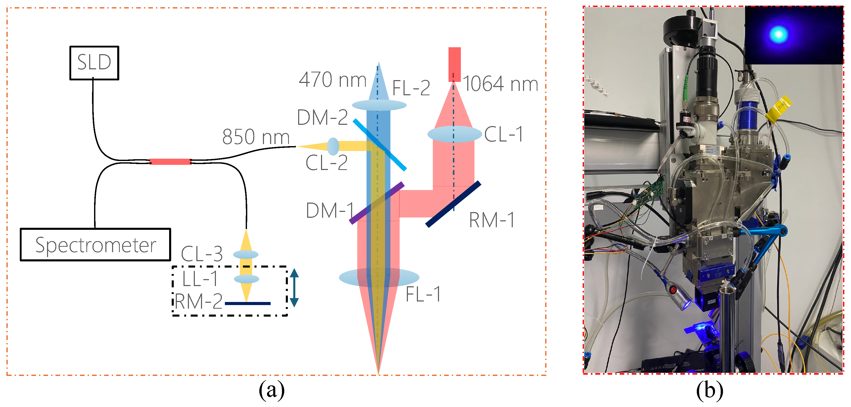
2. System
3. Efficient Depth-Tracking
3.1. Depth-Tracking Algorithm
3.2. Parallel Computing Design
4. Live Control Test
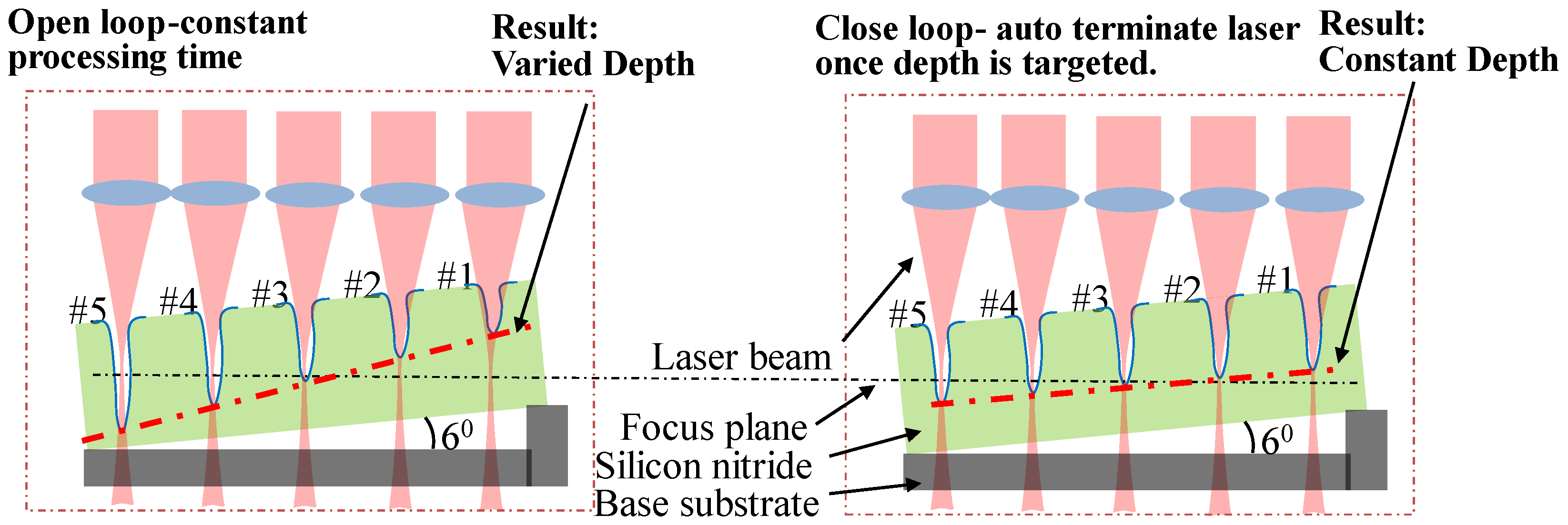
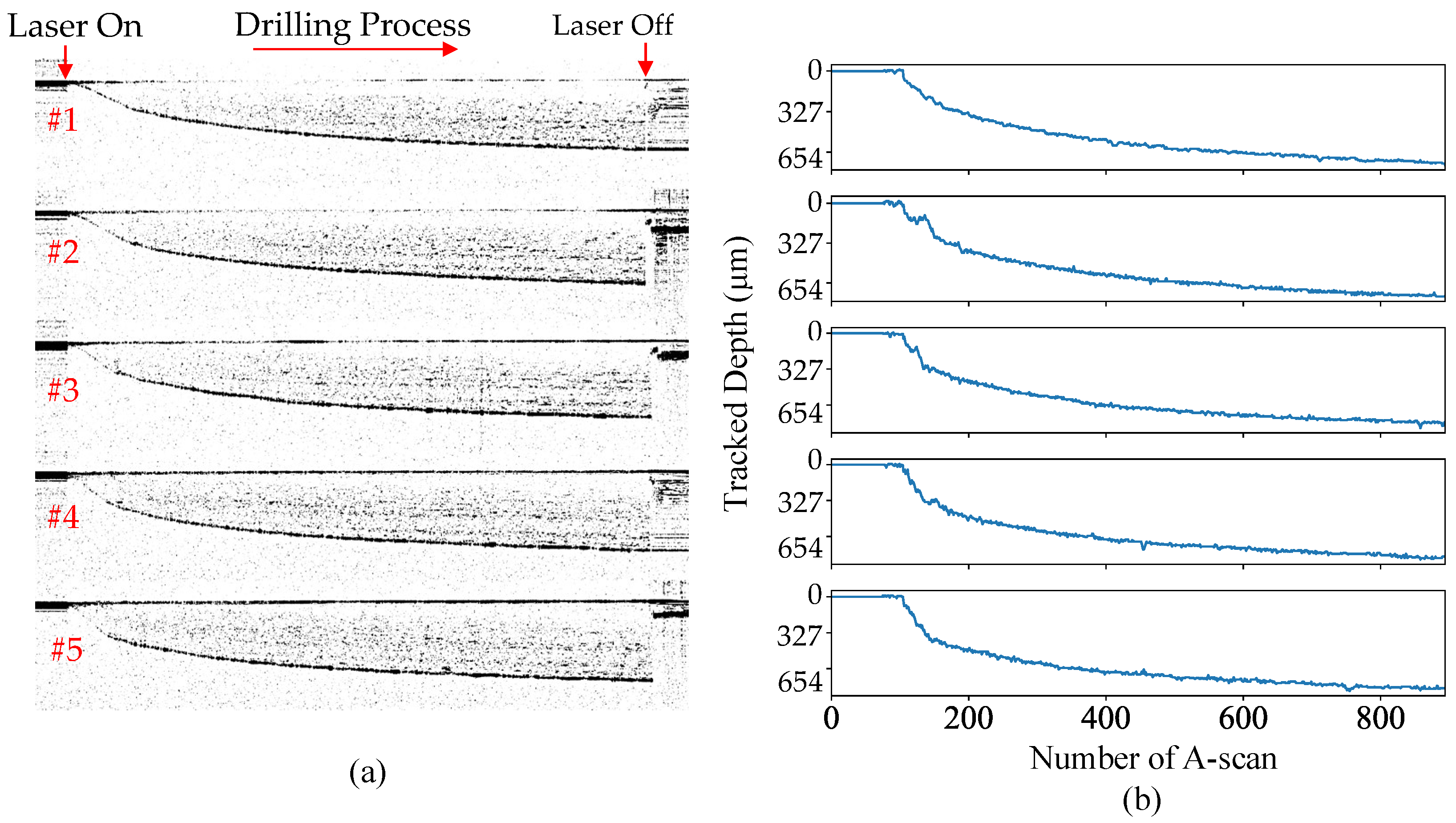
4.1. Drill Hole at Different Offsets without Control
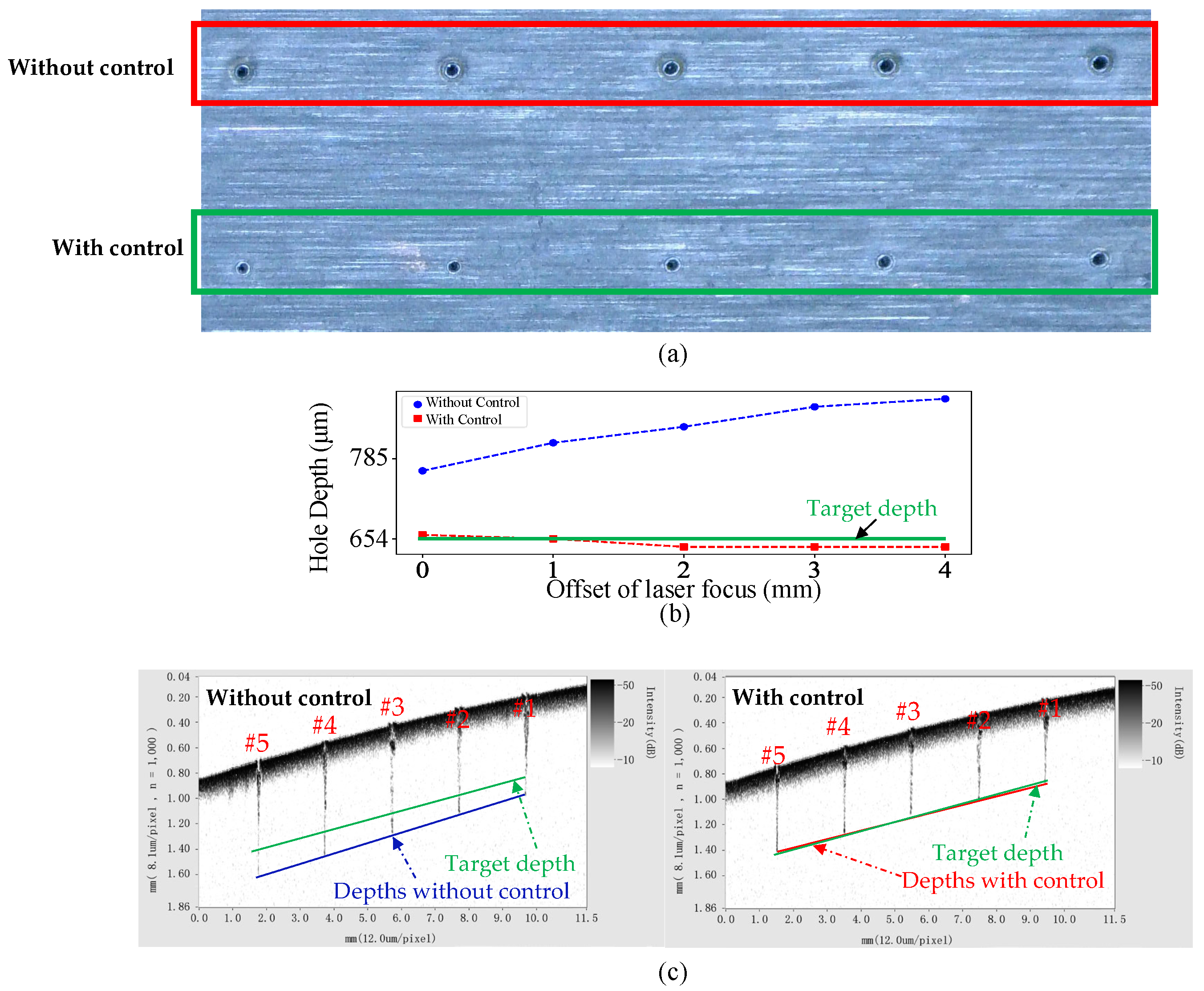
4.2. Drill Hole at Different Offsets with Control
5. Conclusions
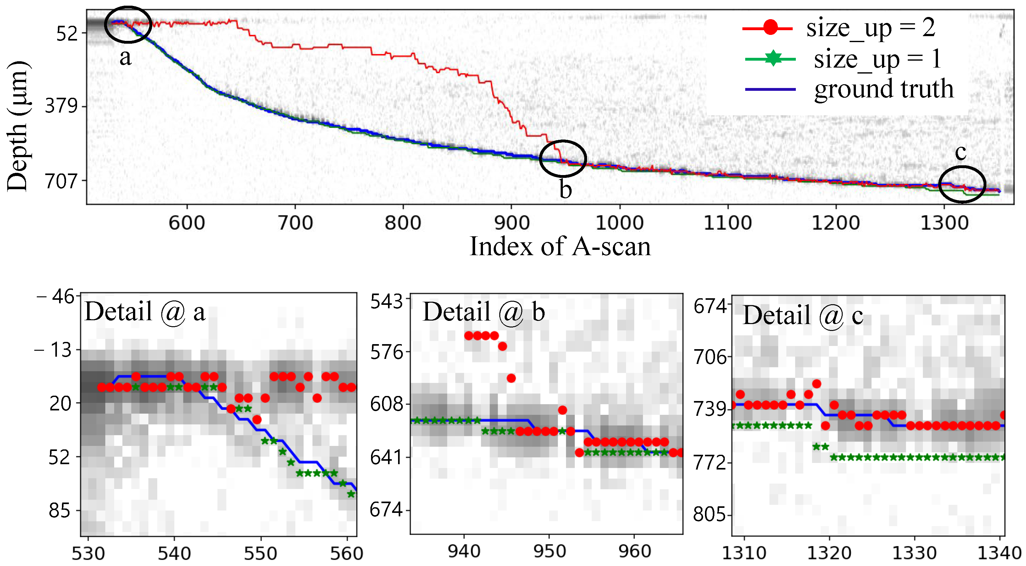
- The computationally heavy FFT involved in biological volume OCT imaging is saved by a depth-tracking algorithm given the two truths of the drilling process that only one interface exists and the interface moves smoothly from one A-scan to the next one. The proposed tracking algorithm expedited the computing speed by six times to 3 k A-scan/s.
- The feedback control rate is further secured by parallelizing the capturing of fringe patterns and the processing of the tracking algorithm in FPGA. Experiments demonstrated that the computing speed of the FPGA reached no less than 187.970 k A-scan/s and stayed stable with various sizes of processing blocks. It is fast enough to conduct live processing for the vast majority of laser drilling processes.
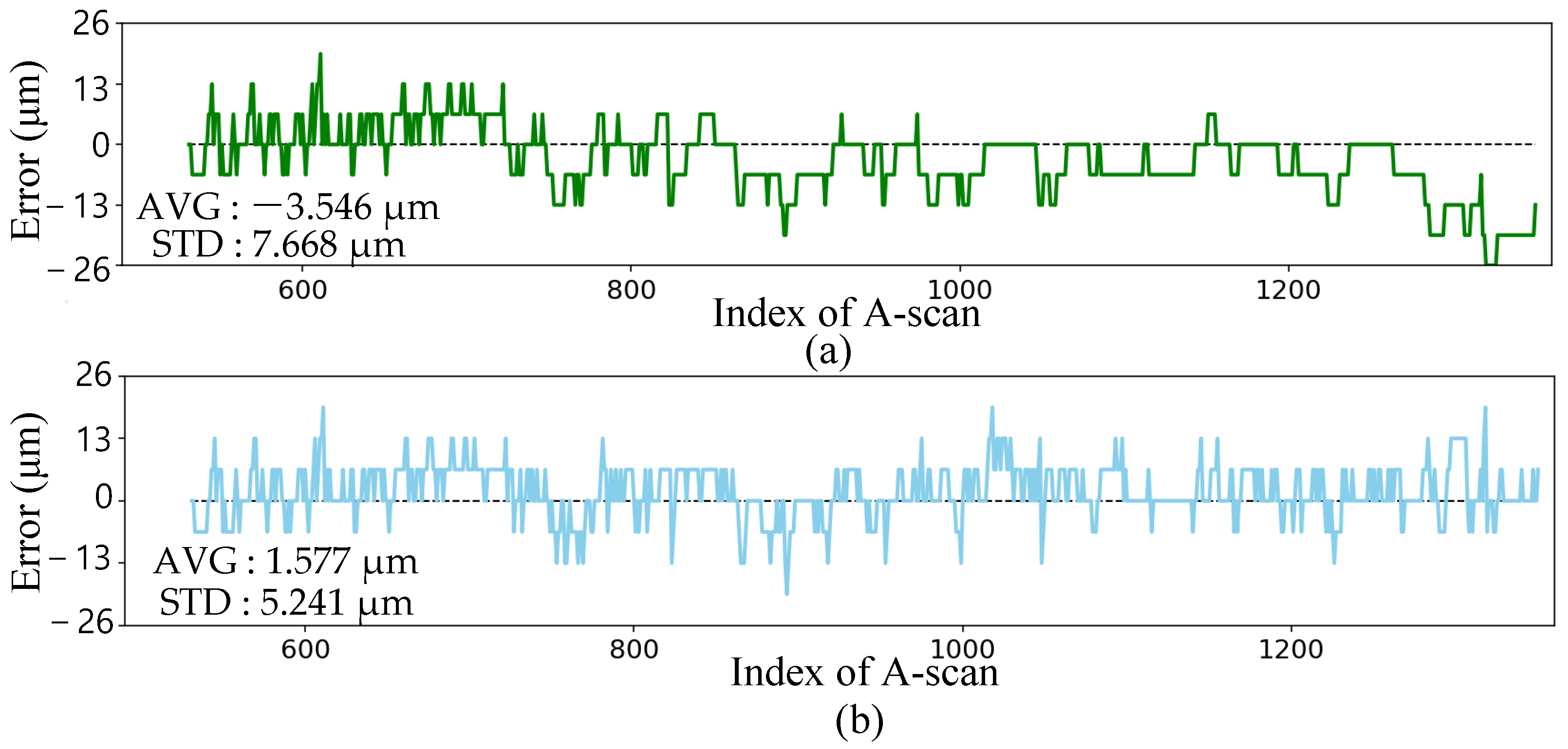
- The test on probe card hole drilling by using the control system shows the capacity of correcting the depths to a target depth within an averaged error of 6.5 m and STD of 8.5 m, which is a huge improvement compared to the hole depths with an averaged error of 179.3 m and STD of 41.9 m without control, showing the good performance of the built control system in achieving the targeted depth.
Author Contributions
Funding
Institutional Review Board Statement
Informed Consent Statement
Data Availability Statement
Acknowledgments
Conflicts of Interest
References
- Chu, W.S.; Kim, C.S.; Lee, H.T.; Choi, J.O.; Park, J.I.; Song, J.H.; Jang, K.H.; Ahn, S.H. Hybrid manufacturing in micro/nano scale: A review. Int. J. Precis. Eng.-Manuf.-Green Technol. 2014, 1, 75–92. [Google Scholar] [CrossRef]
- Choi, W.C.; Ryu, J.Y. Fabrication of a guide block for measuring a device with fine pitch area-arrayed solder bumps. Microsyst. Technol. 2012, 18, 333–339. [Google Scholar] [CrossRef]
- Chatterjee, S.; Mahapatra, S.S.; Xu, J.; Brabazon, D. Influence of parameters on performance characteristics and defects during laser microdrilling of titanium alloys using RSM. Int. J. Adv. Manuf. Technol. 2023, 129, 4569–4587. [Google Scholar] [CrossRef]
- Jia, X.; Dong, J.; Chen, Y.; Wang, H.; Zhu, G.; Kozlov, A.; Zhu, X. Nanosecond-millisecond combined pulse laser drilling of alumina ceramic. Opt. Lett. 2020, 45, 1691–1694. [Google Scholar] [CrossRef] [PubMed]
- Jia, X.; Chen, Y.; Liu, L.; Wang, C. Combined pulse laser: Reliable tool for high-quality, high-efficiency material processing. Opt. Laser Technol. 2022, 153, 108209. [Google Scholar] [CrossRef]
- Jia, X.; Li, K.; Li, Z.; Wang, C.; Chen, J.; Cui, S. Multi-scan picosecond laser welding of non-optical contact soda lime glass. Opt. Laser Technol. 2023, 161, 109164. [Google Scholar] [CrossRef]
- Webster, P.J.; Leung, B.Y.; Joe, X.; Anderson, M.D.; Hoult, T.P.; Fraser, J.M. Coaxial real-time metrology and gas assisted laser micromachining: Process development, stochastic behavior, and feedback control. In Proceedings of the Micromachining and Microfabrication Process Technology XV, San Francisco, CA, USA, 26 January 2010; SPIE: Bellingham, WA, USA, 2010; Volume 7590, pp. 15–24. [Google Scholar]
- Lin, C.H.; Powell, R.A.; Jiang, L.; Xiao, H.; Chen, S.J.; Tsai, H.L. Real-time depth measurement for micro-holes drilled by lasers. Meas. Sci. Technol. 2010, 21, 025307. [Google Scholar] [CrossRef]
- Zhang, Z.; Wang, W.; Jiang, R.; Zhang, X.; Xiong, Y.; Mao, Z. Investigation on geometric precision and surface quality of microholes machined by ultrafast laser. Opt. Laser Technol. 2020, 121, 105834. [Google Scholar] [CrossRef]
- Chen, X.; Xu, Y.; Chen, N.K.; Shy, S.; Chui, H.C. In-situ depth measurement of laser micromachining. Photonics 2021, 8, 493. [Google Scholar] [CrossRef]
- Wang, C.S.; Hsiao, Y.H.; Chang, H.Y.; Chang, Y.J. Process Parameter Prediction and Modeling of Laser Percussion Drilling by Artificial Neural Networks. Micromachines 2022, 13, 529. [Google Scholar] [CrossRef]
- Lv, J.; Dong, X.; Wang, K.; Duan, W.; Fan, Z.; Mei, X. Study on process and mechanism of laser drilling in water and air. Int. J. Adv. Manuf. Technol. 2016, 86, 1443–1451. [Google Scholar] [CrossRef]
- Kumar, D.; Gururaja, S. Investigation of hole quality in drilled Ti/CFRP/Ti laminates using CO2 laser. Opt. Laser Technol. 2020, 126, 106130. [Google Scholar] [CrossRef]
- Lim, D.W.; Kim, M.; Choi, P.; Yoon, S.J.; Lee, H.T.; Kim, K. Hole Depth Prediction in a Femtosecond Laser Drilling Process Using Deep Learning. Micromachines 2023, 14, 743. [Google Scholar] [CrossRef] [PubMed]
- Saif, Y.; Yusof, Y.; Latif, K.; Kadir, A.Z.A.; binti lliyas Ahmed, M.; Adam, A.; Hatem, N.; Memon, D.A. Roundness Holes’ Measurement for milled workpiece using machine vision inspection system based on IoT structure: A case study. Measurement 2022, 195, 111072. [Google Scholar] [CrossRef]
- Ho, C.C.; Li, G.H. Study on the measurement of laser drilling depth by combining digital image relationship measurement in aluminum. Materials 2021, 14, 489. [Google Scholar] [CrossRef] [PubMed]
- Webster, P.J.; Joe, X.; Leung, B.Y.; Anderson, M.D.; Yang, V.X.; Fraser, J.M. In situ 24 kHz coherent imaging of morphology change in laser percussion drilling. Opt. Lett. 2010, 35, 646–648. [Google Scholar] [CrossRef]
- Hasegawa, S.; Fujimoto, M.; Atsumi, T.; Hayasaki, Y. In-process monitoring in laser grooving with line-shaped femtosecond pulses using optical coherence tomography. Light. Adv. Manuf. 2022, 3, 427–436. [Google Scholar] [CrossRef]
- Lin, J.; Zhong, S.; Zhang, Q.; Zhong, J.; Nsengiyumva, W.; Peng, Z. Swept-source optical coherence vibrometer: Principle and applications. IEEE Trans. Instrum. Meas. 2022, 71, 7002209. [Google Scholar] [CrossRef]
- Holder, D.; Weber, R.; Graf, T.; Onuseit, V.; Brinkmeier, D.; Förster, D.J.; Feuer, A. Analytical model for the depth progress of percussion drilling with ultrashort laser pulses. Appl. Phys. A 2021, 127, 302. [Google Scholar] [CrossRef]
- Sun, T.; Fan, Z.; Sun, X.; Ji, Y.; Zhao, W.; Cui, J.; Mei, X. Femtosecond laser drilling of film cooling holes: Quantitative analysis and real-time monitoring. J. Manuf. Process. 2023, 101, 990–998. [Google Scholar] [CrossRef]
- Ho, C.C.; Chang, Y.J.; Hsu, J.C.; Chiu, C.M.; Kuo, C.L. Optical emission monitoring for defocusing laser percussion drilling. Measurement 2016, 80, 251–258. [Google Scholar] [CrossRef]
- Xie, X.; Zhang, Y.; Huang, Q.; Huang, Y.; Zhang, W.; Zhang, J.; Long, J. Monitoring method for femtosecond laser modification of silicon carbide via acoustic emission techniques. J. Mater. Process. Technol. 2021, 290, 116990. [Google Scholar] [CrossRef]
- Subasi, L.; Gokler, M.I.; Yaman, U. A comprehensive study on water jet guided laser micro hole drilling of an aerospace alloy. Opt. Laser Technol. 2023, 164, 109514. [Google Scholar] [CrossRef]
- Krause, T.J.; Allen, T.R.; Fraser, J.M. Self-witnessing coherent imaging for artifact removal and noise filtering. Opt. Lasers Eng. 2022, 151, 106936. [Google Scholar] [CrossRef]
- Ji, Y.; Grindal, A.W.; Webster, P.J.; Fraser, J.M. Real-time depth monitoring and control of laser machining through scanning beam delivery system. J. Phys. Appl. Phys. 2015, 48, 155301. [Google Scholar] [CrossRef]
- Fleming, T.G.; Clark, S.J.; Fan, X.; Fezzaa, K.; Leung, C.L.A.; Lee, P.D.; Fraser, J.M. Synchrotron validation of inline coherent imaging for tracking laser keyhole depth. Addit. Manuf. 2023, 77, 103798. [Google Scholar] [CrossRef]
- Webster, P.J.; Wright, L.G.; Mortimer, K.D.; Leung, B.Y.; Yu, J.X.; Fraser, J.M. Automatic real-time guidance of laser machining with inline coherent imaging. J. Laser Appl. 2011, 23, 022001. [Google Scholar] [CrossRef]


| Block Size A-Scans | PC + FFT | PC + Tracking | FPGA + Tracking |
|---|---|---|---|
| 1 A | 0.069 k | 2.513 k | 187.970 k |
| 10 A | 0.335 k | 2.816 k | 190.876 k |
| 100 A | 0.534 k | 3.172 k | 191.172 k |
| 1000 A | 0.562 k | 3.299 k | 191.201 k |
Disclaimer/Publisher’s Note: The statements, opinions and data contained in all publications are solely those of the individual author(s) and contributor(s) and not of MDPI and/or the editor(s). MDPI and/or the editor(s) disclaim responsibility for any injury to people or property resulting from any ideas, methods, instructions or products referred to in the content. |
© 2024 by the authors. Licensee MDPI, Basel, Switzerland. This article is an open access article distributed under the terms and conditions of the Creative Commons Attribution (CC BY) license (https://creativecommons.org/licenses/by/4.0/).
Share and Cite
Zhao, J.; Zhang, C.; Ding, Y.; Bai, L.; Cheng, Y. Efficient Depth Measurement for Live Control of Laser Drilling Process with Optical Coherence Tomography. Photonics 2024, 11, 743. https://doi.org/10.3390/photonics11080743
Zhao J, Zhang C, Ding Y, Bai L, Cheng Y. Efficient Depth Measurement for Live Control of Laser Drilling Process with Optical Coherence Tomography. Photonics. 2024; 11(8):743. https://doi.org/10.3390/photonics11080743
Chicago/Turabian StyleZhao, Jinhan, Chaoliang Zhang, Yaoyu Ding, Libing Bai, and Yuhua Cheng. 2024. "Efficient Depth Measurement for Live Control of Laser Drilling Process with Optical Coherence Tomography" Photonics 11, no. 8: 743. https://doi.org/10.3390/photonics11080743