Abstract
In this work, a current and magnetic field sensor is proposed and experimentally demonstrated utilizing a fiber-optic Mach–Zehnder interferometer (MZI) structure. In our setup, one of the interferometer arms is coated with magnetic nanoparticles. The MZI comprises a laser source emitting an optical signal, split by a coupler into two signals propagated by a reference fiber and a sensor fiber. The sensing fiber is encased in cobalt ferrite (CoFe2O4). Upon exposure to a magnetic field, CoFe2O4 induces vibration in the fiber, modifying the sensor’s transmission and causing an imbalance between the optical signals of the interferometer arms. This enables us to evaluate the sensor performance regarding sensitivity, accuracy, and saturation. The nanoparticles were synthesized using the protein sol–gel method, resulting in an average crystallite size of 8, 27, and 67 nm for 623, 773, and 1073 K, respectively. Sample characterizations were conducted through X-ray fluorescence, X-ray diffraction, VSM magnetic measurements, and Mössbauer spectroscopy for further analysis of the performance. The sensor exhibited a linear response, achieving a maximum regression between 93.0% and 98.6% across all sample points in the 0 to 150 Oe range, with an output power of approximately 20 dBm, correlated with the applied magnetic field. Sensitivity was measured at 1.15, 0.93, and 1.41 dB/Oe. Previous studies have correlated the horizontal width of the hysteresis loop with sensor saturation. However, by employing a different coating in this work, we complement these findings by demonstrating that the sensor does not saturate if the maximum applied field is smaller than the hysteresis loop width.
1. Introduction
The development of new materials in the 21st century is crucial to meet market demands, with a particular emphasis on magnetic materials. Magnetite (Fe3O4) has been known for its magnetic properties since ancient times [1]. However, a significant breakthrough occurred in 1825 with H. Oersted’s discovery of generating magnetic fields by electric current. This discovery led to numerous subsequent discoveries, theories, and applications related to magnetism, thus driving the development of magnetic materials. Interestingly, most of these materials and their applications are primarily derived from three elements: iron, cobalt, and nickel. These materials play essential roles in many aspects of modern life, from navigation to communication and medicine [2].
There has been a significant increase in interest in the use of nanoparticles in the manufacture of sensors across various industries in recent years, including electronics, magnetism, biomedical, pharmaceuticals, cosmetics, energy, and catalysis. Areas of industry benefiting most from nanotechnology include the development of new functional materials, micro- and nanoscale processing, production of innovative products, and the creation of nanosensors for security purposes [3]. Nanoparticles have dimensions in the nanometric order (nm = m), but can vary in size up to approximately 100 nm [4]. On the other hand, optical sensors are becoming increasingly popular for measuring a variety of physical parameters in diverse applications. This includes measuring temperature, electric current, and magnetic fields [5,6]. Optical sensors are particularly valuable for innovation in monitoring systems in various technological areas, and find application in monitoring the condition of bridges and ships [7] and physicochemical parameters [8], among other examples [9]. An optical sensor is defined as a device that converts light signals into electronic signals.
Sensors based on optical fibers, or fiber-optic sensors, are widely used in various engineering applications, thanks to scientific–technological advances in the 1960s. These sensors were originally developed to meet the demands of telecommunications, and have expanded to a variety of uses through different techniques and for different purposes. Their ability to detect a wide range of physical parameters, such as light intensity, displacement, temperature, pressure, rotation, sound, deformation, magnetic field, radiation, flow, chemical analysis, vibration, and others, makes them attractive solutions for application in various devices [10,11,12,13,14].
Fiber-optic sensors, especially those using interferometry, offer significant advantages over conventional sensors [15]. These sensors are capable of performing highly accurate measurements on a variety of physical or chemical parameters, making them ideal for developing promising devices. The advantages of the optical magnetic field sensor include easy implementation, immunity to electromagnetic interference, suitability for challenging environments, and configurations tailored to specific applications [5]. The use of nanoparticles in conjunction with optical sensors has aroused great interest in measuring different parameters. Some studies in the literature on current and magnetic field sensors stand out. For example, ref. [5] proposed a sensor using a Mach–Zehnder interferometer in optical fibers, incorporating Nickel Ferrite (NiFe2O4) nanoparticles with an average crystallite size of 72 nm, calcined at 1000 °C. In the same way, [12] developed a magnetic field sensor using NiFe2O4 nanoparticles in a Mach–Zehnder interferometer in optical fibers. This study investigated the effect of crystallite size (3.3 nm, 51.9 nm, and 74.3 nm) at different temperatures (300 °C, 600 °C, and 800 °C).
The characteristics of nanoparticles, especially the crystallite size, play a crucial role in magnetic field measurements when used in optical-fiber sensors, which motivated the development of this work. The objective of this study is to verify how a Mach–Zehnder interferometer in optical fibers coated with nanoparticles of CoFe2O4, synthesized by the protein sol–gel method [16], at different temperatures (350 °C, 500 °C, and 800 °C), influences the performance of the magnetic sensor according to the crystallite size.
2. Materials and Methods
2.1. Synthesis of CoFe2O4 Nanoparticles
The synthesis of CoFe2O4 nanoparticle was conducted using the protein sol–gel method, a variation of the traditional sol–gel method that employs hydrolysate gelatin as an organic precursor. The reagents used included Fe( · 9H2O (iron III nitrate nonahydrate) and Co( ·6H2O (cobalt II nitrate hexahydrate), along with hydrolyzed gelatin from the brand SIGMA-ALDRICH.
The nanoparticles were subjected to thermal treatments for 4 h at different temperatures: 623 K (T350), 773 K (T500), and 1073 K (T800). Following this process, a portion of the powder was separated to perform X-ray diffraction (XRD). Subsequently, with the identification of the CoFe2O4 phase, characterizations were carried out using vibrating sample magnetometer (VSM), Mössbauer spectroscopy (MS), and X-ray fluorescence (XRF).
X-ray diffraction of the samples was conducted using a conventional X-ray diffractometer (Rigaku D/MAX-B) with Bragg–Brentano geometry. The device features a 185 mm goniometer radius and 0.02 degrees step , and is equipped with a Cu tube and various slits: a 1-degree scattering slit, two Soller slits, a 1-degree divergence slit, and a 0.3 mm receiving slit. X-ray photon counting is performed using a scintillation detector (NaI). Operating parameters include a 40 kV acceleration potential and 25 mA filament current. The X-ray tube emits and radiation with wavelengths of 1.54050 Åand 1.54443 Å, respectively.
The chemical analysis of the elements present in the samples was performed using a ZSXMini II-Rigaku X-ray fluorescence spectrometer. The equipment operated at 40 kV and 1.2 mA, with a Palladium (Pd) tube. The VSM measurements were performed at room temperature using a vibrating sample magnetometer whose magnetic field ranged from −12 kOe to +12 kOe. The MS was measured at room temperature using a SEECo spectrometer, model W302, with a radioactive source diffused in a rhodium matrix. It was then adjusted with NORMOS software version 1995, employing the hyperfine field distribution method.
2.2. Description of the MZI Sensor Experimental Setup
The Mach–Zehnder sensor works by splitting a beam of light into two separate optical paths, which are later recombined. The resulting interference, whether constructive or destructive, depends on the phase differences caused by the physical quantity being measured. This sensitive technique enables the sensor to detect small changes in these quantities, converting them into visible variations in the light interference pattern [12]. In the experimental setup presented, a fiber-optic sensor employs a Mach–Zehnder interferometer to monitor alternating current and magnetic fields, as illustrated in Figure 1.
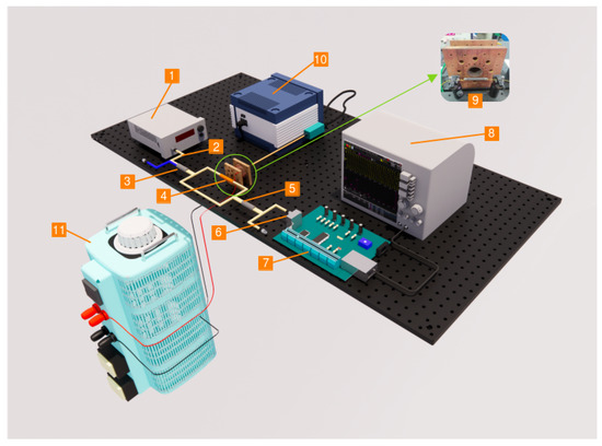
Figure 1.
Mach–Zehnder interferometer-based fiber-optic sensor configuration.
The experiment is organized as follows: a portable laser source (unit 1) emits light with a wavelength of 1550 nm and an optical power of 398.1 W. This light is then guided through a single-mode fiber. The optical signal within the system is divided by a 3 dB coupler (unit 2), directing it into two separate optical-fiber arms. The sensor component (unit 4) is in one of these arms, encased incobalt ferrite (CoFe2O4), with a region surrounded by nanoparticles. The other arm is composed of a conventional optical fiber. Signals from both arms are subsequently recombined using a second 3 dB coupler (unit 5). The signal analysis is performed at the interferometer output for measurement purposes.
The signal captured by the photodiode (unit 6) is processed on the electronic board (unit 7) through a specific circuit designed to amplify and filter the signal before being analyzed on the oscilloscope (unit 8). This electronic board is connected to both the oscilloscope and a multimeter, allowing for precise measurement of electrical voltage values. The magnetic field is generated by the varying electric current passing through a coil (unit 9), inducing a signal in the sensor element through this magnetic field. This field is then measured by a Teslameter (unit 10).
On the other hand, the optical fiber with nanoparticles is tensioned by a support attached to an optical bench, maintaining a fixed distance of 2 cm between the sensor element and the coil. A variac (unit 11) is used to power the coil and create a variable magnetic field to be detected by the sensor, with an alternating current variation injected into the coil ranging from 1 to 10 A, with a step of 1 A. The intensity of this magnetic field is controlled by the circulating current in the coil, whose values are monitored by an ammeter connected to one of the connection wires. This magnetic field is influenced by the frequency of the electrical grid, and interacts with the magnetic nanoparticles present in the optical fiber, causing bends in the fiber and resulting in phase differences. The nanoparticles are encapsulated in the optical fiber using a plastic tube sealed on both sides with a sponge and fixed to the fiber with glue to ensure the system’s integrity.
It is important to highlight the initial optical phase difference between the two arms and how it is controlled. Theoretically, there should be no phase difference but, in practical experiments, small differences are inevitable due to imperfections in the components. High-quality components, such as precision couplers and optical fibers with rigorously measured lengths, are used to minimize this difference, making it irrelevant for the analysis of the results.
No specific polarization control is applied, as the lasers use emitted polarized light, and the signals from the fibers are compared considering this initial polarization. Due to the short lengths of the interferometer arms, the effects of polarization variation and arm length imbalance are minimized, ensuring an accurate evaluation of the interferometric data.
3. Results
3.1. Characterization of Nanoparticles
The results obtained by XRF are presented in Table 1. It is important to highlight that the nanoparticles were synthesized using the protein sol–gel method, resulting in high-quality samples initially studied by both XRF and XRD techniques. XRF analysis revealed an excess of material that did not form the desired phase, as indicated by stoichiometric calculations. These calculations showed values that did not correspond to the expected 1:2 ratio, as shown in Table 2. This discrepancy in stoichiometry can be attributed to the low calcination temperature, among other factors involved in the synthesis process. The results indicated that iron and cobalt are the main elements present in the CoFe2O4 sample at different calcination temperatures; however, they are in low concentrations and were not identified in the crystalline phases by the XRD technique.

Table 1.
XRF analysis of CoFe2O4 nanoparticles.
Table 2.
Refined parameters using the Rietveld method for CoFe2O4 synthesized at T350, T500, and T800, including lattice parameters; SP secondary phase, crystallite size calculated by the Sherrer equation ().
Figure 2 presents the X-ray diffraction (XRD) refinement patterns for CoFe2O4 samples synthesized at 673 K (T350), 773 K (T500), and 1073 K (T800), using the Rietveld method [17]. This method is essential for determining unit cell parameters and identifying the crystalline phases present.
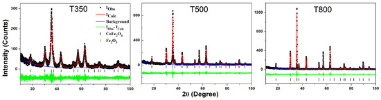
Figure 2.
Rietveld refinement for the T350, T500, and T800 samples. XRD patterns of nanoparticles synthesized using the protein-assisted sol–gel method at various temperatures (black circles). The calculated pattern obtained from the Rietveld refinement is shown as a red line, with the green line indicating the difference between experimental and calculated intensities.
At all synthesis temperatures, the main diffraction peaks of the samples can be indexed based on a cubic face-centered spinel structure, belonging to the Fdm space group. This structure is typical of spinel materials, ensuring structural stability and specific magnetic properties. The presence of spurious iron oxide (Fe2O3) phases is observed in the samples synthesized at 1073 K, being attributed to the partial thermal decomposition of CoFe2O4. Additionally, the main peaks of these samples can be indexed based on the cubic face-centered spinel structures corresponding to the Fdm and Imma space groups, indicating a possible structural distortion caused by the high temperature. These results demonstrate the robustness of the CoFe2O4 spinel structure under different synthesis conditions, while also revealing its sensitivity to high temperatures, resulting in impurities and structural distortions.
The results of the structural refinement using the Rietveld method are presented in Table 2. The average crystallite size was calculated using the Scherrer formula , where represents the full width at half maximum (FWHM) in radians, adjusted for instrumental line broadening, is the Bragg angle, K is a dimensionless shape factor, and represents the radiation wavelength.
The accuracy of the refinements was assessed using the quality parameters and the reliability factors and . As indicated in Table 3, the crystallite size calculated using the Scherrer formula shows an increase in crystallite size with the increase in calcination temperature. There is a growth in crystallite size from 8 nm at T350 to 27 nm at T500 and 67 nm at T800.
Table 3.
The parameter () is the magnetic field variation, () is the output power variation, a is the slope of the line and b the intercept, is the correlation coefficient, is the inclination angle of the line, and S is the sensitivity.
3.2. Mössbauer Spectroscopy
The Mössbauer spectroscopy measurements were conducted at room temperature. The Mössbauer spectra of the CoFe2O4 samples calcined at different temperatures (T350, T500, and T800) are shown in Figure 3.
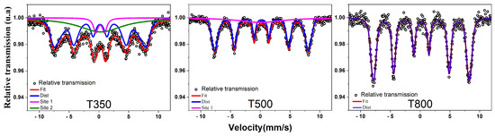
Figure 3.
Mössbauer spectra of CoFe2O4 nanoparticles synthesized at temperatures of 623 K (T350), 773 K (T500), and 1073 K (T800).
The Mössbauer spectrum of the sample treated at T350 revealed three distinct subspectra, a doublet (Site 1), a broad singlet (Site 2), and a distribution of sextets. These subspectra indicate a transition from the superparamagnetic regime to the ferrimagnetic regime of cobalt ferrite, likely due to an increase in the particle size of the material. Based on the isomer shift () and quadrupole splitting () values observed in the doublet, it can be inferred that the iron is present as in both octahedral and tetrahedral sites, which are characteristic of ferrites.
The spectra analysis of samples treated at different temperatures reveals significant changes in the magnetic behavior of cobalt ferrite, influenced by the presence of ions. The spectrum of the sample treated at T500 presented a broad singlet with low intensity and a distribution of sextets, suggesting that the transition from the superparamagnetic to the ferrimagnetic regime is still in progress. This behavior can be attributed to the ions, which play a crucial role in the magnetic structure of cobalt ferrite. According to [18,19], the ions have uncanceled magnetic moments which strongly interact with the ions, influencing the magnetic properties of the materials. In contrast, the spectrum of the sample treated at T800 showed a well-defined distribution of sextets, indicating that the transition from the superparamagnetic to the ferrimagnetic regime has already occurred at this temperature. The literature [20] on magnetic materials suggests that this transition is related to the increase in particle size during the calcination process. X-ray diffraction techniques confirm that the growth of particles with increasing temperature results in particles large enough that thermal agitation no longer disrupts the alignment of magnetic dipoles.
3.3. Vibrating Sample Magnetometer
The magnetization measurements as a function of the magnetic field were conducted at room temperature, as presented in Figure 4.
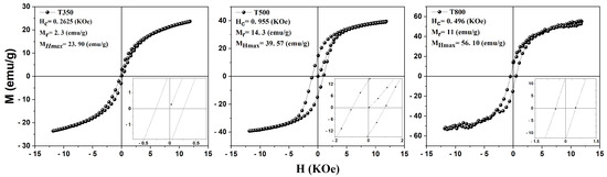
Figure 4.
Magnetic hysteresis loops for the T350, T500, and T800 samples at room temperature.
An interesting fact about this series of samples is that none of them exhibit superparamagnetic behavior, as they all have a considerable coercive field. On the other hand, the literature reports that CoFe2O4 can be superparamagnetic when the particle size is around 4.6 nm; the thermal energy of the medium is sufficient at this size range to overcome the magnetocrystalline energy barrier of this material [21]. Table 3 presents the main parameters obtained from the magnetic measurements of the CoFe2O4 samples. It is observed that the maximum field magnetizations of the samples increase with rising temperature, from 23.90 emu/g at T350 to 56.10 emu/g at T800. This increase in maximum field magnetizations occurs due to the growth in particle size. The coercive field exhibits a rapid increase with the rise in particle size from T350 to T500, but the coercivity decreases at T800, a behavior which has already been analyzed in the literature [22]. The same occurs with the remnant magnetizations, which decrease with increasing temperature from T500 to T800.
3.4. Experimental Result and Discussion
After characterizing the nanoparticles, it can be concluded, through Rietveld refinement, that the lattice parameter increases as the calcination temperature rises, going from 8.359(6) Å at 623 K, to 8.382(4) Å at 773, and 8.392(7) Å at 1073 K (Table 2). A similar trend was observed in the crystallite size, calculated using the Scherrer equation, ranging from 8 nm to 27 nm and 67 nm, respectively.
The increase in calcination temperature promotes greater atomic diffusion and crystalline restructuring, resulting in the crystallite growth. This explains the increase in crystallite size as the calcination temperature rises. The lattice parameter expansion can be attributed to the relief of internal stresses and the possible incorporation of atoms into the crystal lattice, which occur at higher temperatures.
The T350, T500, and T800 nanoparticles were applied to the MZI sensor for microstructural and magnetic analyses. Signal modulation at the sensor’s output occurs due to the interference between optical fields traversing the detection and reference arms. The alternating electrical current in the coil generates an alternating magnetic field in the sensor arm, which contains ferrimagnetic nanoparticles. These nanoparticles respond to the magnetic field, causing the sensor arm to oscillate in sync with it, thus altering the optical signal path and resulting in varying path lengths.
Interference between the optical signal in the detection arm (with nanoparticles) and the reference arm (without nanoparticles) leads to modulation in the amplitude of the output signal. Physically, the difference in optical path lengths, caused by the sensor arm’s oscillation, induces a phase variation between the signals in the two arms. This phase variation interferes constructively or destructively, modulating the output signal amplitude of the sensor.
Several tests, as shown in Figure 5, were conducted to evaluate the sensor’s efficacy and performance under different magnetic field conditions. When a magnetic field is applied, the CoFe2O4 nanoparticles vibrate and transmit this vibration to the optical fiber, causing a variation in the optical path length of the light and resulting in phase modulation. Without the magnetic field, there is no phase difference between the reference and sensor arms. However, with the magnetic field, the nanoparticles’ vibration alters the optical path, recorded at the interferometer’s output as an oscillating sinusoidal signal.
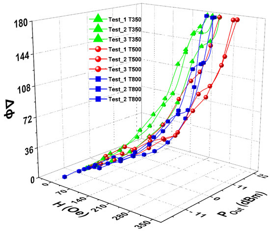
Figure 5.
Optical power variation in the signal as a function of the magnetic field for T350, T500, and T800.
The interference between the two recombined beams in the interferometer depends on the phase difference () between them. The phase difference is a crucial measure for understanding how the modulation of the magnetic field affects the detected signal. The formula used to calculate the phase difference is as follows:
where is the input signal power and is the output signal power. This formula derives from the principle of interference, where the phase difference between two light beams results in variations in the intensity observed at the interferometer output. The phase difference () is calculated from the measured powers of the input and output signals. The formula considers the relationship between the measured power and the resulting interference, allowing the quantification of the phase change induced by the vibration of the nanoparticles. Phase modulation is a fundamental aspect for analyzing the sensor’s sensitivity to the magnetic field. The ability to detect and quantify these phase variations allows for an accurate assessment of the sensor’s performance under different experimental condition [23].
The analysis of this signal was performed using Fast Fourier Transform (FFT) directly on the oscilloscope, identifying a peak at 120 Hz, whose intensity allows the quantification of the phase modulation induced by the magnetic field. It was observed that the maximum power recorded in each test did not exceed 20 dBm. In some cases, the power remained nearly constant when the applied magnetic field exceeded 200 Oe. These results indicate that the sensor maintains its efficacy even under relatively intense magnetic field conditions, highlighting its potential for applications in environments with significant magnetic field variations. It is important to note that the power mentioned in the article refers to the electrical signal power corresponding to the oscillation frequency of 120 Hz, not the optical power. The FFT, performed with the oscilloscope, converts the signal from the time domain to the frequency domain, allowing the measurement of signal intensity in terms of frequency.
A specific analysis of the output power in dBm (decibel milliwatt) for the T350, T500, and T800 nanoparticles revealed different behaviors. For the T350 sample, the output power increases with the magnetic field up to 150 Oe, where it then stabilizes. The output power in the tests with the T500 sample consistently increases with the applied field until it reaches 280 Oe, after which the power tends to stabilize. In the tests with the T800 sample, the output power exhibits a linear behavior relative to the applied field, with stabilization occurring around 264 Oe.
The slope of the lines obtained through the linear regression method in the analysis of the MZI sensor’s response can be used to evaluate the sensor’s sensitivity, as shown in Figure 6. The slope reflects the variation in the sensor’s output in response to changes in the applied magnetic field, providing an accurate measure of sensitivity.
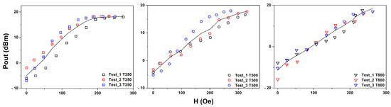
Figure 6.
Fit by linear regression method of the T350, T500, and T800 sensor signals.
In the specific case of the MZI sensor we are studying, sensitivity is defined by the relationship between the variation in the sensor output and the variation in the input parameter , such as electric current or magnetic field. Technically, the sensitivity of the sensor is expressed as the slope of the characteristic response curve, /. This means that sensitivity is determined by the variation in output power relative to a specific change in the physical input parameter.
Sensitivity is a critical parameter in sensor performance, with high sensitivity being highly desirable in practical applications as it enables more precise detection of small environmental changes. The sensitivity of the sensor (S) can be calculated by the change in output power (P) due to the variation in the applied magnetic field (H). The minimum and maximum output power values, and , are considered for two different applied magnetic fields, and , as shown in the expression below.
Table 3 presents the sensor sensitivity in the optical-fiber experiments conducted at T350, T500, and T800. It is observed that the sensor sensitivity does not exhibit a linear relationship with crystallite size at T500, being lower compared to T350 and T800. This phenomenon can be attributed to Mössbauer characterization, which indicates a gradual transition from the superparamagnetic regime to the ferrimagnetic regime in this sample. This suggests that the magnetic moments are disordered, making their orientation difficult in the presence of an external field. Additionally, VSM measurements showed a disproportionate increase at T500 compared to T350, indicating greater difficulty in orienting these moments. These results affect the sensor response, which exhibited reduced sensitivity at T500 compared to temperatures T350 and T800.
The sensitivity values obtained in this study exceed those reported in the literature. As demonstrated by Li Zeng et al. [24], who proposed and demonstrated an optical-fiber magnetic field sensor with an intensity modulation based on the Mach–Zehnder Interferometer (MZI) and magnetic fluid, achieving a maximum sensitivity to the magnetic field intensity of 0.563 dB/Oe. Another instance is the vector magnetic field fiber-optic sensor presented by Zhang et al. [25], which combines Fiber Bragg Gratings (FBGs) with magnetic fluids (MFs), achieving a sensitivity to the magnetic field intensity of 0.143 dB/Oe in the linear range of 60 to 110 Oe. Moreover, the sensitivity of sample T500, the minimum value obtained in this study, surpasses the values mentioned previously in the literature.
Araújo et al. [12] conducted a study in which they proposed the hypothesis that an increase in the magnetization of the samples would result in a greater oscillation of the fiber, leading to an amplified output power, with saturation occurring when the magnetization of the samples reached very high levels. However, upon analyzing the responses of the sensors under the available experimental conditions, it was found that the applied field reached its maximum value in the range of 200 to 300 Oe for all sensors, with none of them reaching saturation. Therefore, based on the findings of this experiment, the hypothesis of Araújo et al. [12] was not confirmed, as saturation did not occur in the tests.
An alternating magnetic field was used in the experiments with the MZI sensor, causing the fiber oscillation to resemble a hysteresis loop, varying between positive and negative magnetic field values. Thus, analyzing the magnetic field based on the VSM measurements of the samples can provide an explanation for the occurrence or non-occurrence of saturation in the sensor’s output power, considering the conditions described in the literature.
Another condition proposed by the same authors, using current and magnetic field sensors, can be confirmed through testing these sensors. The authors suggest a relationship between the sensor’s saturation and the magnetic field range of the samples’ hysteresis cycle, as presented in Figure 7. This relationship establishes that saturation of the output power occurs when the magnetic field applied to the sensor exceeds the magnetic field range of the sample’s hysteresis cycle. Conversely, sensor saturation does not occur when the magnetic field applied to the sensor is below the magnetic field range of the hysteresis cycle.
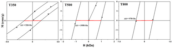
Figure 7.
Magnification of the central part of the hysteresis loops of the T350, T500, and T800 samples.
Figure 7 and Table 3 demonstrate that the magnetic field range of the hysteresis cycle for each sample is higher than the maximum field applied to the sensor. The magnetic field range of the hysteresis cycle for the T350 sample was 520 Oe, while the maximum field applied to the sensor was only 251 Oe. The T500 sample presented a magnetic field range of 1950 Oe, being six times greater than the maximum field applied to the sensor, which reached 282 Oe. Finally, the T800 sample showed a decline in the magnetic field range of the hysteresis cycle, reaching 970 Oe, still higher than the maximum field applied to the sensor, which was 254 Oe.
Thus, the study is validated, confirming non-saturation of the sensor when using cobalt ferrite as the sensing element. Cobalt ferrite proved efficient in maintaining measurement integrity even when subjected to magnetic fields higher than those expected to saturate the sensor. This result highlights the robustness and suitability of cobalt ferrite for applications requiring high precision in magnetic field detection, ensuring the reliability of the collected data.
4. Conclusions
The performance of current and alternating magnetic field sensors was analyzed, utilizing the Mach–Zehnder interferometer structure with cobalt ferrite nanoparticles as the sensing element. This study enabled confirming previously reported results in the literature and also explored new considerations. The sensor demonstrated linear behavior in all samples within the regions between 0 and 150 Oe, with an output power value of approximately 20 dBm, subsequently tending towards a constant behavior.
The results corroborate previous studies on the use of nanoparticles in interferometric sensors, relating the horizontal width of the hysteresis loop to the sensor’s saturation. By examining the horizontal width and the maximum field applied to the sensor, it was possible to predict whether the samples would saturate. The sensor showed sensitivity in the T350 and T800 samples, consistent with the concept that the sensor’s sensitivity increases with the nanoparticle’s magnetization, as the sample’s magnetization increases with the crystallite size. However, the results for the T500 sample did not follow this trend.
Author Contributions
All authors contributed to the study conception and design. Material preparation, data collection, and analysis were performed by F.W.C.d.V. The first draft of the manuscript was written by Y.M.C., G.d.F.G. and J.S.d.A. The authors J.M.S., M.R.A., L.Q.R. and M.A.R.M. made significant contributions to the studies and understanding of material characteristics. On the other hand, L.S.P.M., J.I.S.M. and I.K.A.d.S. were responsible for the development and refinement of the optical setup. All authors commented on previous versions of the manuscript. All authors have read and agreed to the published version of the manuscript.
Funding
The authors are grateful to the Brazilian Agencies CAPES PDPG (Grant numbers 88887.707631/2022-00), CNPq (Grant numbers: 408071/2021-8), FACEPE, and FINEP for financial support.
Institutional Review Board Statement
Not applicable.
Informed Consent Statement
Not applicable.
Data Availability Statement
Data can be made available upon request.
Acknowledgments
The authors thank the LRX laboratory (UFC) and Fotonic Laboratory (IFCE) for the sample preparation support, and the LAMOp laboratory of UERN (State University of Rio Grande do Norte).
Conflicts of Interest
The authors declare no conflicts of interest.
References
- Ganapathe, L.S.; Mohamed, M.A.; Mohamad Yunus, R.; Berhanuddin, D.D. Magnetite (Fe3O4) nanoparticles in biomedical application: From synthesis to surface functionalisation. Magnetochemistry 2020, 6, 68. [Google Scholar] [CrossRef]
- Valenzuela, R. Novel applications of ferrites. Phys. Res. Int. 2012, 2012, 591839. [Google Scholar] [CrossRef]
- Duran, N. Nanotecnologia: Introdução, Preparação e Caracterização de Nanomateriais e Exemplos de Aplicação; Artliber: São Paulo, Brazil, 2006. [Google Scholar]
- Fechine, P.B.A. Avanços no Desenvolvimento de Nanomateriais; Imprensa Universitária: Fortaleza, Brazil, 2020. [Google Scholar]
- Souza, F.C.N.; Maia, L.S.P.; Medeiros, G.M.; Miranda, M.A.R.; Sasaki, J.M.; Guimaraes, G.F. Optical Current and Magnetic Field Sensor Using Mach-Zehnder Interferometer with Nanoparticles. IEEE Sens. J. 2018, 18, 7998–8004. [Google Scholar] [CrossRef]
- Maia, L.S.P.; Miranda, M.A.R.; de Souza, I.M.X.; de Assis, B.C.P.; Rocha, D.S.; Sasaki, J.M.; de Alexandria, A.R.; de Freitas Guimarães, G. Optical current and magnetic field sensor using multimodal interference in fiber optics with carbon steel. IEEE Sens. J. 2022, 22, 12877–12885. [Google Scholar] [CrossRef]
- Friebele, E.J. Fiber Bragg grating strain sensors: Present and future applications in smart structures. Opt. Photonics News 1998, 9, 33. [Google Scholar] [CrossRef]
- Frazão, O.; Falate, R.; Fabris, J.; Santos, J.L.; Ferreira, L.A.; Araújo, F. Optical inclinometer based on a single long-period fiber grating combined with a fused taper. Opt. Lett. 2006, 31, 2960–2962. [Google Scholar] [CrossRef] [PubMed]
- Liu, J. Fuzzy modularity and fuzzy community structure in networks. Eur. Phys. J. B 2010, 77, 547–557. [Google Scholar] [CrossRef]
- Grattan, K.T.V.; Sun, T. Fiber optic sensor technology: An overview. Sens. Actuators A Phys. 2000, 82, 40–61. [Google Scholar] [CrossRef]
- Berkovic, G.; Shafir, E. Optical methods for distance and displacement measurements. Adv. Opt. Photonics 2012, 4, 441–471. [Google Scholar] [CrossRef]
- Araújo, M.R.; Maia, L.S.; Miranda, M.A.; Martínez-Camejo, Y.; Sasaki, J.M.; Guimarães, G.F. Optimization of nanoparticles for application in optical sensors. Sens. Actuators A Phys. 2024, 366, 114923. [Google Scholar] [CrossRef]
- Krohn, D.A.; MacDougall, T.; Mendez, A. Fiber Optic Sensors; Spie Press Bellingham: Bellingham, WA, USA, 2014. [Google Scholar]
- Zhou, X.; Li, X.; Li, S.; An, G.W.; Cheng, T. Magnetic field sensing based on SPR optical fiber sensor interacting with magnetic fluid. IEEE Trans. Instrum. Meas. 2018, 68, 234–239. [Google Scholar] [CrossRef]
- Lee, B.H.; Kim, Y.H.; Park, K.S.; Eom, J.B.; Kim, M.J.; Rho, B.S.; Choi, H.Y. Interferometric fiber optic sensors. Sensors 2012, 12, 2467–2486. [Google Scholar] [CrossRef] [PubMed]
- Maia, A.d.O.G.; Oliveira, F.G.S.; Cordeiro, C.H.N.; Teixeira, E.S.; da Silva, E.B.; Soares, J.M.; de Vasconcelos, I.F.; Sasaki, J.M.; Dumelow, T. Synthesis of CoFe2O4 superparamagnetic nanoparticles using a rapid thermal processing furnace with halogen lamps. J. Sol-Gel Sci. Technol. 2021, 99, 527–533. [Google Scholar] [CrossRef]
- Young, R.A. The Rietveld Method; International Union of Crystallography: Chester, UK, 1993; Volume 5. [Google Scholar]
- Chandra, G.; Srivastava, R.; Reddy, V.; Agrawal, H. Effect of sintering temperature on magnetization and Mössbauer parameters of cobalt ferrite nanoparticles. J. Magn. Magn. Mater. 2017, 427, 225–229. [Google Scholar] [CrossRef]
- Gu, Z.; Xiang, X.; Fan, G.; Li, F. Facile synthesis and characterization of cobalt ferrite nanocrystals via a simple reduction-oxidation route. J. Phys. Chem. C 2008, 112, 18459–18466. [Google Scholar] [CrossRef]
- Moumen, N.; Bonville, P.; Pileni, M. Control of the size of cobalt ferrite magnetic fluids: Mössbauer spectroscopy. J. Phys. Chem. 1996, 100, 14410–14416. [Google Scholar] [CrossRef]
- Esharighi, M.; Kameli, P. Magnetic properties of CoFe2O4 nanoparticles prepared by thermal treatment of ball-milled precursors. Curr. Appl. Phys. 2011, 11, 476–481. [Google Scholar] [CrossRef]
- Nogueira, N.A.S.; Utuni, V.H.S.; Silva, Y.C.; Kiyohara, P.K.; Vasconcelos, I.F.; Miranda, M.A.R.; Sasaki, J.M. X-ray diffraction and Mossbauer studies on superparamagnetic nickel ferrite (NiFe2O4) obtained by the proteic sol-gel method. Mater. Chem. Phys. 2015, 163, 402–406. [Google Scholar] [CrossRef]
- Born, M.; Wolf, E. Principles of Optics: Electromagnetic Theory of Propagation, Interference and Diffraction of Light; Elsevier: Amsterdam, The Netherlands, 2013. [Google Scholar]
- Zeng, L.; Sun, X.; Zhang, L.; Hu, Y.; Duan, J. High sensitivity magnetic field sensor based on a Mach-Zehnder interferometer and magnetic fluid. Optik 2022, 249, 168234. [Google Scholar] [CrossRef]
- Zhang, J.; Chen, F.; Wang, R.; Qiao, X.; Chen, H.; Zhang, X. Vector magnetic field measurement based on magnetic fluid and high-order cladding-mode Bragg grating. Opt. Laser Technol. 2021, 143, 107264. [Google Scholar] [CrossRef]
Disclaimer/Publisher’s Note: The statements, opinions and data contained in all publications are solely those of the individual author(s) and contributor(s) and not of MDPI and/or the editor(s). MDPI and/or the editor(s) disclaim responsibility for any injury to people or property resulting from any ideas, methods, instructions or products referred to in the content. |
© 2024 by the authors. Licensee MDPI, Basel, Switzerland. This article is an open access article distributed under the terms and conditions of the Creative Commons Attribution (CC BY) license (https://creativecommons.org/licenses/by/4.0/).