Analysis and Selection of the Optimal Pump Laser Power Density for SERF Co-Magnetometer Used in Rotation Sensing

Abstract

This paper systematically studies the output noise model of the K-Rb-²¹Ne co-magnetometer and proposes the method for determining the optimal pump laser power density. The amplitude-frequency response and the equivalent model for each frequency band are obtained through the transfer function of the co-magnetometer. Based on the established model and considering the power spectral density characteristics of magnetic noise, the output noise equation is formulated. Consequently, the pump laser power density yielding minimal output noise is determined. Both experimental and simulation results indicate that the pump laser power density yielding minimal output noise is greater than the pump laser power density corresponding to the maximum scale factor. Moreover, when the co-magnetometer operates at the pump laser power density corresponding to the minimal output noise, the output noise can be reduced by approximately 25%, and the Allan variance reaches its optimal value. The optimal Allan variance at 180 °C and 190 °C are 0.01395°/h @100 s and 0.01329°/h @100 s, respectively. Therefore, this pump laser power density is designated as the optimal pump laser power density for the co-magnetometer. Finally, simulations are conducted to investigate the variation patterns of the optimal pump laser power density points and the minimum output noise under different density ratios and gas pressures. The theories and methods proposed in this paper provide significant reference value for selecting the optimal pump laser power density and suppressing magnetic noise in co-magnetometers.

1. Introduction

Spin-exchange relaxation-free (SERF) co-magnetometers (CM), due to their ultra-high sensitivity, have been widely used in frontier physical explorations, including tests of Lorentz and CPT symmetry [1], seeking light-axis dark matter [2], and exploration of electric dipole moment [3,4], etc. Simultaneously, this CM is also a highly promising inertial rotation sensor for next-generation inertial navigation system [5,6].

In 2005, the K-³He CM was first proposed and implemented by the Romalis group at Princeton University. And they also highlighted the great potential of the K-³He CM for rotational measurements [7]. Subsequently, CMs based on Cs-¹²⁹Xe and Rb-¹²⁹Xe have been proposed and realized [8,9]. Subsequent research has shown that the sensitivity of a CM used as a sensor for measuring angular velocity is inversely proportional to the gyromagnetic ratio of the noble gas, and the gyromagnetic ratio of ²¹Ne is smaller than that of ³He and ¹²⁹Xe, so the noble gas atoms were replaced with ²¹Ne [10]. In order to reduce polarization gradients and improve the pumping efficiency of noble gas atoms, the hybrid optical pumping technique is adopted. That is, the vapor cell is filled with K and Rb alkali metal atoms, in which the optically thin atoms (K) are directly polarized by the pump laser, and then the polarized K atoms polarize the optically thick atoms (Rb) through spin-exchange collisions. Based on the above research, the K-Rb-²¹Ne CM has been proposed [11,12]. However, the current sensitivity of the SERF CM is far below the theoretical estimate [6]. Therefore, it is necessary to conduct an in-depth analysis of the errors and perform detailed optimizations to achieve better performance.

On the one hand, previous research primarily establish the output noise equation of the CMs based on the steady-state solution of the Bloch equation. This approach not only overlooks the frequency response of the CM but also focused primarily on probe laser noise [13,14]. Since magnetic noise, which can affect the atomic polarization state, is neglected, previous studies have concluded that when the pumping rate equals the spin-destruction rate, the scale factor reaches its maximum value, and sensitivity is optimized [15,16]. On the other hand, although our research team considered the impact of magnetic noise, the analysis typically focuses on the response amplitude at a specific fixed frequency as the magnetic field response coefficient. Research efforts are directed toward reducing this magnetic field response coefficient, neglecting characteristics such as the power spectral density of the magnetic noise [17,18,19,20]. Therefore, research in the area of modeling the output noise of the system and thus determining the optimal pump laser power density point, taking into account the magnetic noise power spectral density characteristics, is urgently needed.

This paper systematically studies the output noise model and the method for determining the optimal pump laser power density in the K-Rb-²¹Ne CM. The structure of this paper is arranged as follows. In Section 1, the amplitude-frequency response and the equivalent model of each frequency band are obtained through the transfer function of the CM. And the noise output model is established by combining the power spectral density characteristics of magnetic noise. Section 2 introduces the experimental setup of K-Rb-²¹Ne CM used in this paper. Section 3 first verifies the equivalent models for each frequency band. Then, it calculates the output noise using measured parameters such as the equivalent magnetic field of electron spin polarization at different vapor cell temperatures and pump light power densities. The calculation results are verified through theoretical simulations. Section 4 simulates the variation patterns of the optimal pump light power density and the minimum output noise under different density ratios and pressures. Section 5 is the conclusion.

2. Theory

2.1. Principle of the SERF CM

Although our setup includes two types of alkali metal atoms, the rapid spin-exchange collisions between K and Rb atoms result in the two types of atoms having the same dynamic process. Therefore, the dynamic process of the SERF CM can be described using the following Bloch equations [21,22].

$$\begin{array}{cc}\hfill {\displaystyle \frac{\partial {\mathbf{P}}^{\mathbf{e}}}{\partial t}}& ={\displaystyle \frac{{\gamma }_e}{Q\left({\mathbf{P}}^{\mathbf{e}}\right)}}\left({\mathbf{B}}^c+\lambda M^n{\mathbf{P}}^{\mathbf{n}}+\mathbf{L}\right)\times {\mathbf{P}}^{\mathbf{e}}-\Omega \times {\mathbf{P}}^{\mathbf{e}}+{\displaystyle \frac{R_p{\mathbf{s}}^{\mathbf{p}}+R_m{\mathbf{s}}^{\mathbf{m}}+R_{se}^{en}{\mathbf{P}}^{\mathbf{n}}}{Q\left({\mathbf{P}}^{\mathbf{e}}\right)}}\hfill \\ \hfill & -{\displaystyle \frac{{\left[R_2^e,R_2^e,R_1^e\right]}^T}{Q\left({\mathbf{P}}^{\mathbf{e}}\right)}}·{\mathbf{P}}^{\mathrm{e}},\hfill \\ \hfill {\displaystyle \frac{\partial {\mathbf{P}}^{\mathbf{n}}}{\partial t}}=& {\gamma }_n\left({\mathbf{B}}^c+\lambda M^e{\mathbf{P}}^e\right)\times {\mathbf{P}}^{\mathbf{n}}-\Omega \times {\mathbf{P}}^{\mathbf{n}}+R_{se}^{ne}{\mathbf{P}}^{\mathbf{e}}-{\left[R_2^n,R_2^n,R_1^n\right]}^T·{\mathbf{P}}^{\mathbf{n}},\hfill \end{array}$$

(1)

where, ${\mathbf{P}}^{\mathbf{e}}={\left[P_x^e,P_y^e,P_z^e\right]}^T$ and ${\mathbf{P}}^{\mathbf{n}}={\left[P_x^n,P_y^n,P_z^n\right]}^T$ represent electron-spin polarization and nuclear-spin polarization, respectively. ${\gamma }_e$ and ${\gamma }_n$ are the gyromagnetic ratios of the electron spins and nuclear spins, respectively. $Q\left({\mathbf{P}}^{\mathbf{e}}\right)$ is the slowing-down factor of the electron spins, which is a function of the electron-spin polarization. ${\mathbf{B}}^{\mathrm{c}}$ is the externally applied compensation magnetic field vector. ${\mathbf{B}}^{\mathbf{n}}=\lambda M^n{\mathbf{P}}^{\mathbf{n}}$ and ${\mathbf{B}}^{\mathrm{e}}=\lambda M^e{\mathbf{P}}^{\mathrm{e}}$ are the equivalent magnetic fields of the nuclear spins and electron spins, respectively, where $M^n$ and $M^e$ are the magnetization vectors when the nuclear spin and electron spin are fully polarized. $\lambda =2{\kappa }_0/3$ is the geometric factor that includes the Fermi contact enhancement factor ${\kappa }_0$. The light shift $\mathbf{L}$ can be considered as a virtual magnetic field. $\Omega$ is the rotational velocity vector relative to inertial space. $R_p$ and $R_m$ are the pumping rates of the pump light and probe light, respectively. ${\mathbf{s}}^{\mathbf{p}}$ and ${\mathbf{s}}^{\mathbf{m}}$ are the photon spin polarization vectors of the pump light and probe light, respectively. $R_{se}^{en}$ and $R_{se}^{ne}$ denote the spin-exchange collisions rate between electron spins and nuclear spins. $R_2^e$, $R_2^n$ and $R_1^n$, $R_1^e$ are the transverse relaxation rates and longitudinal relaxation rates of the nuclear spins and electron spins, respectively.

In Equation (1), K and Rb atoms are considered as one type of alkali metal atom. Therefore, relevant parameters can be defined using the density ratio $D_r$ of the two atoms, where $D_r=n_K/n_{Rb}$. The specific parameters for the electron spins are as follow [16]

$$\begin{array}{cc}\hfill & R_p=\varsigma {\displaystyle \frac{L_p{r}_{e}cf}{h{v}_K}}{\displaystyle \frac{\Gamma /2}{{\left(v_K-v_{K0}\right)}^2+{(\Gamma /2)}^2}},\hfill \\ \hfill & R_{se}^{en}={\sigma }_{se}\overline{v}{n}_{Ne},\hfill \\ \hfill & R_{sd}^e=\varsigma R_{sd}^K+\xi R_{sd}^{Rb}\hfill \\ \hfill & R_1^e=R_p+R_{sd}^e,\hfill \\ \hfill & R_{se}^{rel}=\varsigma R_{se}^{rel-K}+\xi R_{se}^{rel-Rb}\hfill \\ \hfill & R_2^e=R_1^e+R_{se}^{rel},\hfill \\ \hfill & P_z^e={\displaystyle \frac{R_p}{R_1^e}},\hfill \\ \hfill & B^e=2\left(\varsigma {\kappa }_{k-Ne}{n}_k+\xi {\kappa }_{Rb-Ne}{n}_{Rb}\right){\mu }_0{\mu }_e{P}_z^e/3,\hfill \\ \hfill & {\omega }_e={\displaystyle \frac{{\gamma }^e{B}^e}{Q}}.\hfill \end{array}$$

(2)

Here, $\varsigma =D_r/\left(1+D_r\right)$ and $\xi =1/\left(1+D_r\right)$. ${\sigma }_{se}$ is the spin-exchange cross-section. $\overline{\nu }$ is the relative velocity. $n_{Ne}$ is the density of noble gas atoms in the vapor cell. $L_p$ is the pump laser power density. $r_e$ is the electron radius, c is the speed of light in a vacuum, and h is Planck constant. $v_K$ and $v_{K0}$ are the actual frequency of the pump laser and the resonant frequency of K atoms, respectively. $\Gamma$ is the pressure broadening. f is the oscillator strength, with the resonant strengths of the D1 line and D2 line being 1/3 and 2/3, respectively. $R_{sd}^K$ and $R_{sd}^{Rb}$ are the spin-destruction rates for K atoms and Rb atoms, respectively. $R_{se}^{rel-K}$ and $R_{se}^{\mathrm{rel}-Rb}$ are the electron spin-exchange relaxation rates for K atoms and Rb atoms, respectively. ${\mu }_0$ is the vacuum permeability. ${\mu }_B$ is the Bohr magneton. $K_{K-Ne}$ and $K_{Rb-Ne}$ are the Fermi contact enhancement factors for K atoms and Rb atoms with ²¹Ne, respectively. ${\omega }_e$ is the electron resonance frequency.

The parameters related to nuclear spins can be expressed using the following Equations [23,24].

$$\begin{array}{cc}\hfill & R_{se}^{ne}={\displaystyle \frac{n_{Rb}}{n_{Ne}}}{R}_{se}^{en},\hfill \\ \hfill & R_1^n=R_{\mathrm{quad}}^n+R_{sd}^n+R_{se}^{ne},\hfill \\ \hfill & R_2^n=R_1^n+{\displaystyle \frac{1}{V}}{\int }_{\mathrm{volume}}{\displaystyle \frac{8{\gamma }^n{R}^4{\left|{\nabla }_{Bz}\right|}^2}{175D_{Ne-Ne}}}dV,\hfill \\ \hfill & P_z^n={\displaystyle \frac{R_{se}^{ne}}{R_1^n}},\hfill \\ \hfill & B^n=2\left(\varsigma {\kappa }_{k-Ne}+\xi {\kappa }_{Rb-Ne}\right){\mu }_0{n}_{Ne}{P}_z^n/3,\hfill \\ \hfill & {\omega }_n={\gamma }^n{B}^n.\hfill \end{array}$$

(3)

where, $R_{\mathrm{quad}}^n$ is the quadrupole relaxation determined by the density of noble gas atoms. $R_{sd}^n$ is the spin-destruction rates of noble gas atoms. ${\nabla }_{B_z}$ is the magnetic field gradient along the direction of propagation of the pump laser. $D_{Ne-Ne}$ is the diffusion coefficient. R and V are the radius and volume of the vapor cell, respectively. ${\omega }_n$ is the nuclear resonance frequency.

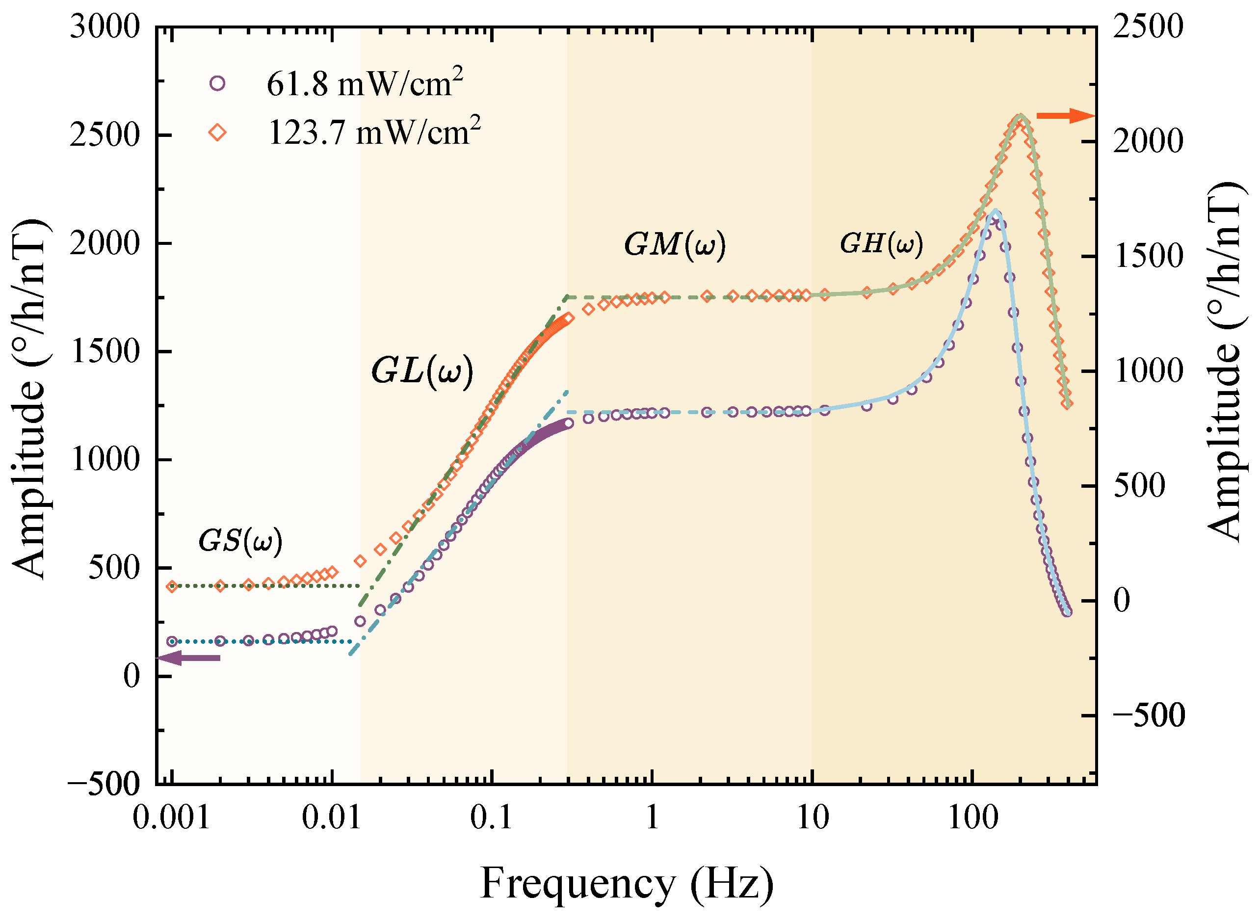
2.2. AC Response Model and Equivalent Models for Each Frequency Band

When a small amplitude transverse magnetic field or angular velocity is applied, the deviation angle of the electron spins longitudinal polarization component $P_z^e$ and the nuclear spins longitudinal polarization component $P_z^n$ from the direction of the pump laser is minimal. Therefore, $P_z^e$ and $P_z^n$ can be considered constants [25]. Based on this assumption, Equation (1) can be simplified into a system of linear equations and can be represented by the following state-space expression:

$$\dot{X}=\mathbf{AX}+\mathbf{CU}.$$

(4)

Here, $\mathbf{X}={\left[P_x^e,P_y^e,P_x^n,P_y^n\right]}^T$ is the state variable and $\mathbf{U}={\left[{\Omega }_x,{\Omega }_y,B_x,B_y\right]}^T$ is the input vector. The state matrix $\mathbf{A}$ is

$$\mathbf{A}=\left[\begin{array}{cccc}-{\displaystyle \frac{R_2^e}{Q}}& {\displaystyle \frac{{\gamma }^e{B}^e}{Q}}& {\displaystyle \frac{R_{se}^{en}}{Q}}& {\displaystyle \frac{{\gamma }^e\lambda M^n{P}_z^e}{Q}}\\ {\displaystyle \frac{{\gamma }^e{B}^e}{Q}}& -{\displaystyle \frac{R_2^e}{Q}}& -{\displaystyle \frac{{\gamma }^e\lambda M^n{P}_z^e}{Q}}& {\displaystyle \frac{R_{se}^{en}}{Q}}\\ R_{se}^{ne}& {\gamma }^n\lambda M^e{P}_z^n& -R_2^n& -{\gamma }^n{B}^n\\ -{\gamma }^n\lambda M^e{P}_z^n& R_{se}^{ne}& {\gamma }^n{B}^n& -R_2^n\end{array}\right],$$

(5)

the input matrix C is given by

$$\mathbf{C}=\left[\begin{array}{cccc}0& -P_z^e& 0& {\displaystyle \frac{P_z^e{\gamma }^e}{Q}}\\ P_z^e& 0& -{\displaystyle \frac{P_z^e{\gamma }^e}{Q}}& 0\\ 0& -P_z^n& 0& P_z^n{\gamma }^n\\ P_z^n& 0& -P_z^n{\gamma }^n& 0\end{array}\right].$$

(6)

Upon obtaining the system’s state matrix, the transfer function matrix of the SERF CM can be given by the following equation

$$\mathbf{G}\left(s\right)={(s\mathbf{I}-\mathbf{A})}^{-1}\mathbf{C}.$$

(7)

where, considering that in our practical experiments, we mainly focus on the projection of electron spin polarization along the x-axis, $\mathbf{G}\left(s\right)$ can be expressed as $\mathbf{G}\left(s\right)=\left[\begin{array}{cccc}{G}_{\Omega x}\left(s\right)\hfill & G_{\Omega y}\left(s\right)\hfill & G_{Bx}\left(s\right)\hfill & G_{By}\left(s\right)\hfill \end{array}\right]$. $\mathbf{I}$ is the identity matrix and s is the complex variable in the transfer function. The primary interference error in the CM comes from the x-axis magnetic field [26], so we focus on the transfer function $G_{Bx}\left(s\right)$. Using Equation (7), $G_{Bx}\left(s\right)$ can be derived as follows

$$G_{Bx}\left(s\right)={\displaystyle \frac{K_{Bx}\left(s+z_{Bx1}\right)\left(s+z_{Bx2}\right)}{\left[{\left(s-{\lambda }_1\right)}^2+{\omega }_1^2\right]\left[{\left(s-{\lambda }_2\right)}^2+{\omega }_2^2\right]}}.$$

(8)

Here,

$$K_{B_x}={\displaystyle \frac{-P_z^e{\gamma }^e\left({\omega }_e+{\omega }_n\right)}{Q}},$$

(9)

$$\begin{array}{cc}\hfill & z_{Bx1}=-R_2^n,\hfill \\ \hfill & z_{Bx2}={\displaystyle \frac{-{\omega }_{e}Q{R}_2^n-{\omega }_n{R}_2^e}{\left({\omega }_e+{\omega }_n\right)Q}}.\hfill \end{array}$$

(10)

$$\begin{array}{cc}\hfill & {\lambda }_1=-{\displaystyle \frac{R_2^e/Q+R_2^n}{2}}+{\displaystyle \frac{1}{2\sqrt{2}}}\sqrt{\sqrt{a^2+b^2}+a},\hfill \\ \hfill & {\lambda }_2=-{\displaystyle \frac{R_2^e/Q+R_2^n}{2}}-{\displaystyle \frac{1}{2\sqrt{2}}}\sqrt{\sqrt{a^2+b^2}+a}.\hfill \end{array}$$

(11)

$$\begin{array}{cc}\hfill & {\omega }_1={\displaystyle \frac{1}{2}}\left({\omega }_e+{\omega }_n\right)+{\displaystyle \frac{1}{2\sqrt{2}}}Sign\left[\mathrm{b}\right]\sqrt{\sqrt{a^2+b^2}-a},\hfill \\ \hfill & {\omega }_2={\displaystyle \frac{1}{2}}\left({\omega }_e+{\omega }_n\right)-{\displaystyle \frac{1}{2\sqrt{2}}}Sign\left[\mathrm{b}\right]\sqrt{\sqrt{a^2+b^2}-a}.\hfill \end{array}$$

(12)

$$\begin{array}{cc}\hfill & a={\left(R_2^e/Q-R_2^n\right)}^2-{\left({\omega }_e-{\omega }_n\right)}^2+4R_{\mathrm{se}}^{\mathrm{ne}}{R}_{\mathrm{se}}^{\mathrm{en}}/Q-4{\omega }_{\mathrm{ne}}{\omega }_{\mathrm{en}},\hfill \\ \hfill & b=-2\left(R_2^e/Q-R_2^n\right)\left({\omega }_e-{\omega }_n\right)-4\left(R_{\mathrm{se}}^{\mathrm{ne}}{\omega }_{\mathrm{ne}}/Q+R_{\mathrm{se}}^{\mathrm{en}}{\omega }_{\mathrm{en}}\right).\hfill \end{array}$$

(13)

After the transfer function $G_{B_x}\left(s\right)$ is known, the amplitude-frequency response model of the system can be obtained by substituting s with $j\omega$ and calculate the modulus.

$$\begin{array}{cc}\hfill \left|G_{B_x}\left(j\omega \right)\right|& =K_{B_x}\sqrt{{\displaystyle \frac{\left({\omega }^2+{z_{Bx1}}^2\right)}{\left[{\left({\lambda }_1^2+{\omega }_1^2-{\omega }^2\right)}^2+{\left(2{\lambda }_1\omega \right)}^2\right]}}}\hfill \\ \hfill & ·\sqrt{{\displaystyle \frac{\left({\omega }^2+z_{Bx2}^2\right)}{\left[{\left({\lambda }_2^2+{\omega }_2^2-{\omega }^2\right)}^2+{\left(2{\lambda }_2\omega \right)}^2\right]}}}.\hfill \end{array}$$

(14)

Equation (14) is complex in form and not conducive to subsequent integral calculations, so it is necessary to construct equivalent models for each frequency band.

When $\omega <R_2^n$, the amplitude-frequency response in this frequency band does not vary with frequency and is mainly determined by the proportional element in Equation (8). By substituting typical parameters and omitting terms with numerical results less than the order of ${10}^{-3}$, the following equation can be derived

$$\left|GS\left(\omega \right)\right|={\displaystyle \frac{P_z^e{\gamma }^e{R}_2^n}{R_2^e{\omega }_n}}.$$

(15)

When $R_2^n<\omega <{\omega }_n$, the amplitude-frequency response in this frequency band increases monotonically with frequency and is mainly dominated by the differential element in Equation (8). At this point, the response of electron spins polarization can be neglected, and the equivalent model in this frequency band can be written as

$$\left|GL\left(\omega \right)\right|={\displaystyle \frac{P_z^e{\gamma }^e\omega }{R_2^e{\omega }_n}}.$$

(16)

When ${\omega }_n<\omega <N_0{\omega }_n$, the amplitude-frequency response in this frequency band also reaches a plateau, mainly determined by two second order oscillation elements in Equation (8). The equivalent model in this frequency band can be expressed as shown in Equation (17),

$$\left|GM\left(\omega \right)\right|={\displaystyle \frac{K_{Bx}}{{\left(R_2^e\right)}^2+{\omega }_e^2}}.$$

(17)

When $\omega >N_0{\omega }_n$, there is an electron resonance peak in this frequency band, mainly dominated by the second order oscillation element related to electron spins polarization in Equation (8). Therefore, the equivalent model in this frequency band is

$$\left|GH\left(\omega \right)\right|={\displaystyle \frac{P_z^e{\gamma }^e}{Q}}{\displaystyle \frac{{\omega }_e}{\sqrt{\left({\left(\omega -{\omega }_e\right)}^2+{\left(R_2^e/Q\right)}^2\right)\left({\left(\omega +{\omega }_e\right)}^2+{\left(R_2^e/Q\right)}^2\right)}}}.$$

(18)

2.3. Output Noise Model

Noise in SERF CMs can be primarily categorized into two types [14]: the first type interacts with atoms, thereby affecting their polarization state, while the second type does not alter atomic polarization but directly couples with the output signal.

The first type of noise is primarily magnetic noise, which mainly includes hysteresis loss noise and eddy current loss noise, each with different power spectral density characteristics [12,27]. The second type of noise is primarily probe background noise, which includes the probe laser polarization, power, ambient temperature, and circuit noise. When considering the effects of both types of noise on the CM, the system’s output signal can be expressed as follows

$$S\left(\omega \right)=K·P_x^e\left(\omega \right)=K·\left[\left|G_{{\Omega }_y}\left(\omega \right)\right|{\Omega }_y\left(\omega \right)+G_{\mathrm{mag}}\left(\omega \right)+N_{bg}\left(\omega \right)\right].$$

(19)

where, $G_{\mathrm{mag}}\left(\omega \right)$ is the magnetically induced noise, and $N_{bg}\left(\omega \right)$ is the equivalent probe background noise. K is the coefficient that converts the transverse component of electron spins polarization $P_x^e$ to voltage, which is generally a constant when the vapor cell parameters, detection light power, frequency, and other factors are fixed.

The bandwidth of the SERF CM is relatively small [28], and during experimental testing, the CM is usually in a stationary state. Therefore, $\left|G_{{\Omega }_y}\left(\omega \right)\right|$ can be replaced with $\left|G_{{\Omega }_y}\left(0\right)\right|$. Thus, the scale factor of the CM for angular rate can be written as

$$K_{\Omega }=K\left|G_{{\Omega }_y}\left(0\right)\right|=K{\displaystyle \frac{P_z^e{\gamma }^e}{R_2^e{\gamma }^n}}.$$

(20)

Combining Equations (19), and (20), the output noise model $N\left(\omega \right)$ can be obtained with a dimension of °/h.

$$N\left(\omega \right)={\displaystyle \frac{K·G_{mag}\left(\omega \right)}{K_{\Omega }}}+{\displaystyle \frac{K·N_{bg}\left(\omega \right)}{K_{\Omega }}}.$$

(21)

The first term in Equation (21) is the magnetically induced output noise, denoted as $G_{\mathrm{mag}}^{\Omega }$.

In SERF CMs, the primary source of magnetic noise is the shielding cylinder used to block the environmental magnetic field. The main factor affecting zero-bias stability is hysteresis loss magnetic noise, which has a noise power spectral density characterized by a 1/f distribution. The power spectral density can be expressed by Equation (22) [12,27,29]

$$S_{\mathrm{mag}}\left(\omega \right)={\left(\delta B_{\mathrm{mag}}\left(\omega \right)\right)}^2/2={\displaystyle \frac{C_{\mathrm{mag}}^2}{2\omega }},$$

(22)

where, $C_{\mathrm{mag}}$ is the hysteresis loss noise coefficient.

The output noise power spectral density and the output noise of this type of magnetic noise after passing through the CM are shown in Equations (23) and (24). In Equations (23), the division by $G_{\Omega y}\left(0\right)$ ensures that the output noise has the unit of °/h. ${\omega }_{up}$ is the upper limit of integration, determined mainly from the magnetic noise power spectral density.

$$S_{\mathrm{mag}}^{\Omega }\left(\omega \right)={\left|G_{B_x}\left(\omega \right)/G_{\Omega y}\left(0\right)\right|}^2{S}_{\mathrm{mag}}\left(\omega \right),$$

(23)

$$G_{\mathrm{mag}}^{\Omega }={\left({\int }_0^{{\omega }_{up}}{S}_{\mathrm{mag}}^{\Omega }\left(\omega \right)d\omega \right)}^{1/2}.$$

(24)

Because the complex form of Equation (24) is not conducive to solving and analyzing, it is necessary to bring the equivalent model of each frequency band into Equation (24) to obtain a simple model for subsequent analysis. Considering that the hysteresis loss magnetic noise power is mainly concentrated in the low-frequency band, so the actual calculation is only need to consider $GS\left(\omega \right)$, $GL\left(\omega \right)$, and $GM\left(\omega \right)$.

$$G_{mag}^{\Omega }={\left(\begin{array}{c}{\int }_{L_m}^{R_2^n}{\left|GS\left(\omega \right)/G_{{\Omega }_y}\left(0\right)\right|}^2{S}_{\mathrm{mag}}\left(\omega \right)d\omega \hfill \\ +{\int }_{R_2^n}^{{\omega }_n}{\left|GL\left(\omega \right)/G_{{\Omega }_y}\left(0\right)\right|}^2{S}_{\mathrm{mag}}\left(\omega \right)d\omega \hfill \\ +{\int }_{{\omega }_n}^{N_0{\omega }_n}{\left|GM\left(\omega \right)/G_{{\Omega }_y}\left(0\right)\right|}^2{S}_{\mathrm{mag}}\left(\omega \right)d\omega \hfill \end{array}\right)}^{1/2}.$$

(25)

Based on the above analysis, the output noise equation $N\left(\omega \right)$ of the SERF CM can be obtained by bringing Equation (25) into Equation (21) as shown below

$$\begin{array}{cc}\hfill N\left(\omega \right)& ={\displaystyle \frac{C_{\mathrm{mag}}}{2}}·\left[\begin{array}{c}{\left({\displaystyle \frac{R_2^n}{{\omega }_n}}\right)}^{2}ln\left(L_m·R_2^n\right)+{\displaystyle \frac{{\omega }_n^2-{\left(R_2^n\right)}^2}{2{\left(B^n\right)}^2}}\hfill \\ +{\left({\displaystyle \frac{{\gamma }^n{\omega }_{e}Q}{R_2^e+{\left({\omega }_{e}Q\right)}^2/R_2^e}}\right)}^{1/2}ln\left(N_0\right)\hfill \end{array}\right]\hfill \\ \hfill & +{\displaystyle \frac{R_2^e{\gamma }^n}{P_z^e{\gamma }^e}}{N}_{bg}\left(\omega \right).\hfill \end{array}$$

(26)

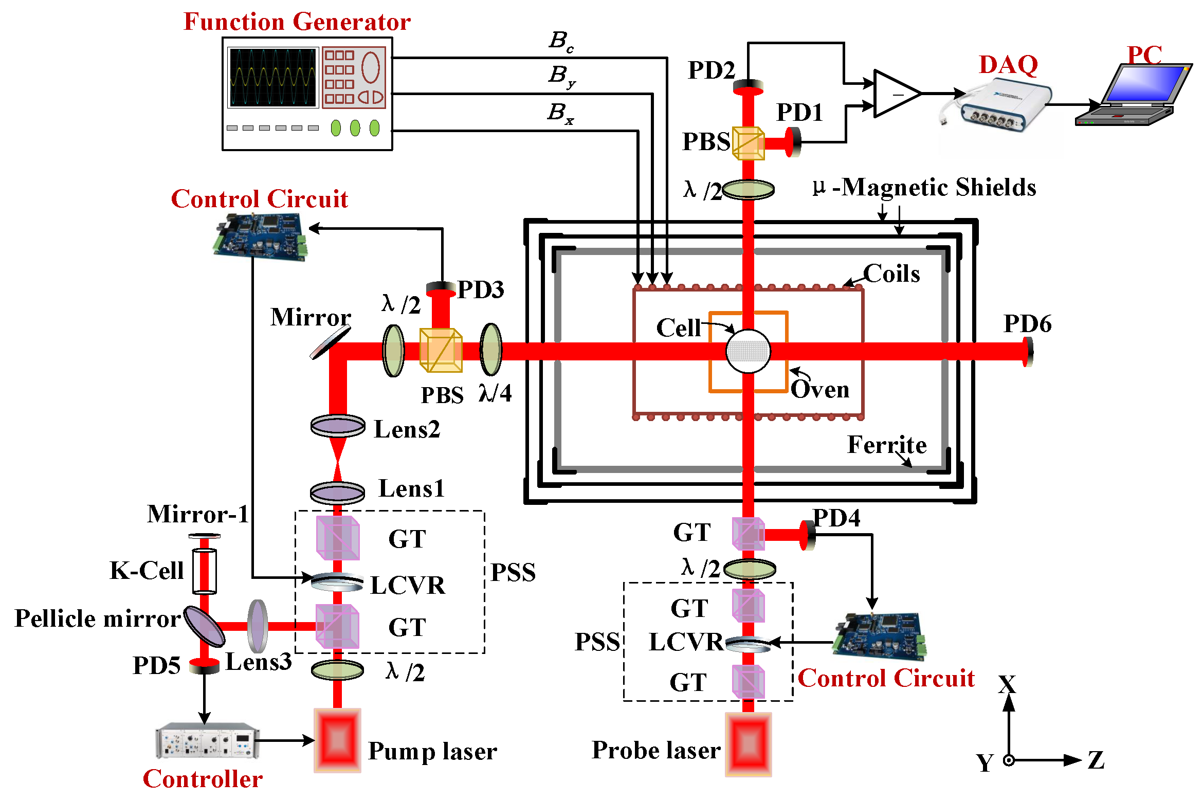
3. Experimental Setup

This experiment is conducted using a K-Rb-²¹Ne CM. The schematic diagram of the CM experimental setup is shown in Figure 1. The sensitive element of this setup is a 4-mm-radius vapor cell made of GE180 silicate glass, containing a mixture of alkali metals (³⁹K, 72.2% ⁸⁵Rb, and 27.8% ⁸⁷Rb), 1 atm of ²¹Ne (70% abundance), and 18 torr of N₂. The vapor cell is installed in a boron nitride oven wrapped with a heating film. The heating film is connected to a circuit control system that includes a power amplification module, capable of generating high-frequency alternating drive currents. The operating temperature of the CM can be set via the host computer of the circuit control system. The test data in this paper are collected at two temperatures: 180 °C and 190 °C. At these temperatures, the vapor cell density ratios are 1/80 and 1/60, respectively. To ensure that the alkali metal atoms operate in the SERF regime, we use a magnetic shielding cylinder composed of two-layers high-permeability $\mu$-metal and one layer of MnZn ferrite to shield the environmental magnetic field. The diameters of the two layers of $\mu$-metal are 128 mm and 104 mm, respectively, with a thickness of 4 mm. The shielding factor of the entire shielding cylinder is approximately 10⁵. Additionally, a triaxial magnetic compensation coil is installed inside the magnetic shielding cylinder, with the coil constant for the transverse axis (x and y-axes) being 0.028 nT/mV and for the longitudinal axis (z-axis) being 0.03467 nT/mV. This coil is driven by a signal generator, which can compensate for residual magnetization and also provide an excitation magnetic field source for the experiment.

The pump beam is emitted by a distributed Bragg reflector (DBR) laser, and its wavelength is locked to the D1 transition line of K atoms (770.108 nm) with the saturation absorption frequency stabilization technology. The pump laser passes through a power stabilization system (PSS), a beam expansion system, and a quarter-wave plate before entering the vapor cell to polarize the alkali metal atoms. The power stabilization system includes a pair of Glan-Taylor prisms (GT), a liquid crystal variable retarder (LCVR), a half-wave plate ($\lambda /2$), a polarizing beam splitter (PBS), a photodiode (PD), and a circuit control system. The pump light power can be set via the power stabilization system. The probe beam is generated by a distributed feedback (DFB) diode laser, with its wavelength tuned 0.3 nm away from the D1 line of Rb atoms to ensure a larger scale factor. After passing through a power stabilization system, it enters the vapor cell to detect the component of the electronic polarization along the x-axis. The entire balanced differential detection module includes a half-wave plate ($\lambda /2$), a polarizing beam splitter (PBS), and two photodetectors (PDs). This module effectively suppresses common-mode noise. All experimental data are ultimately collected by a high-resolution data acquisition system (NI-USB 4431) and transmitted to the host computer for display.

To test the scale factor of CM for angular rate, the CM setup is placed on a uniaxial rate turntable with an accuracy of 0.001°/s. This ensures that the sensitive axis of CM (y-axis) is parallel to the rotation axis of the rate table and oriented upwards.

4. Results and Discussion

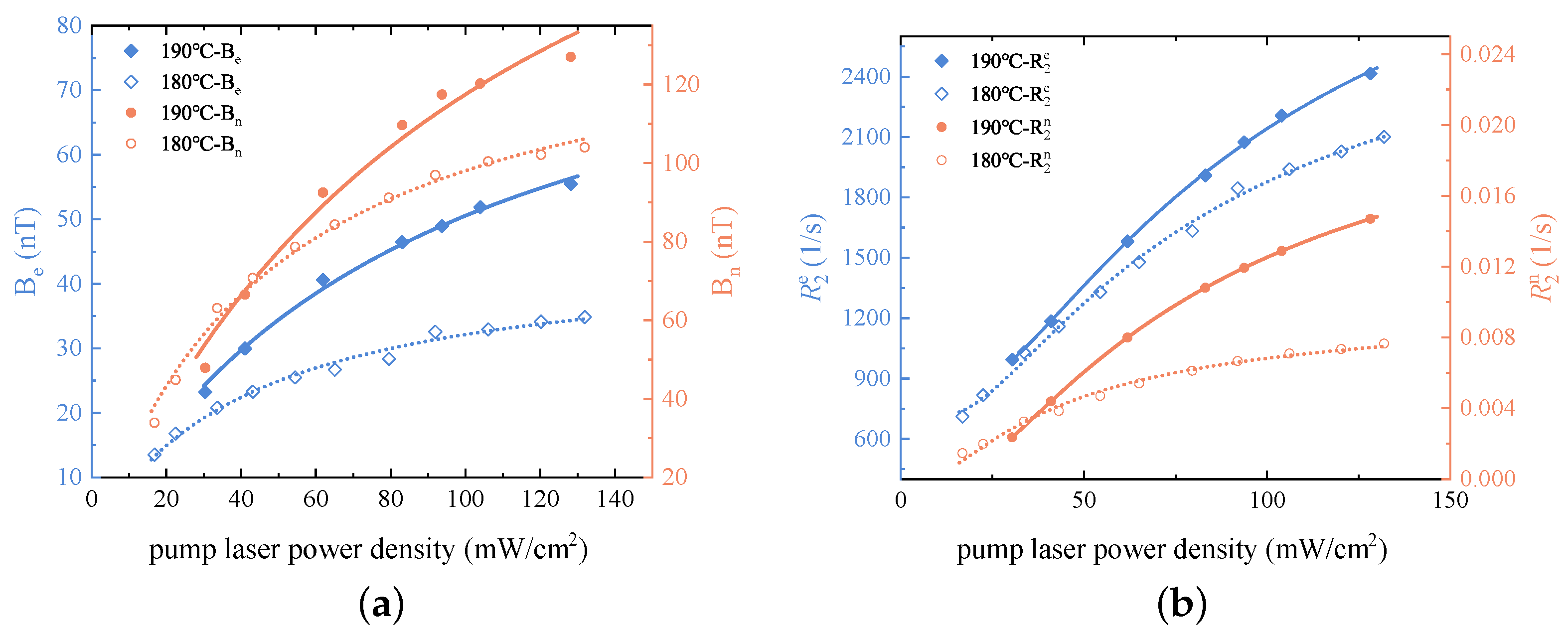
4.1. Parameter Measurements and Equivalent Model Validation

To facilitate the verification of the equivalent model and the calculation of output noise $N\left(\omega \right)$, we first test $B_e$, $B_n$, $R_2^e$, and $R_2^n$ at vapor cell temperatures of 180 °C and 190 °C under different pump laser power densities. $B_n$ can be obtained by finding the minimum response amplitude of the CM to a sinusoidal alternating magnetic field $B_x$, while $B_e$ is equal to $B_z^c-B_n$ [30]. $R_2^e$ can be calculated from the step response parameters of the CM to a magnetic field [31]. $R_2^n$ can be directly measured using the free induction decay (FID) method [32]. The measurement results of these parameters are shown in Figure 2. Figure 2a presents the measurements of $B_e$ and $B_n$, while Figure 2b shows the measurements of $R_2^e$ and $R_2^n$. It is evident that all four parameters increase with the rising pump light power density, which aligns with our anticipated behavior.

By applying a series of 0.5 nT sinusoidal alternating magnetic fields at different frequencies along the x-axis of CM, the output signal can be synchronously demodulated using a lock-in amplifier (Model OE2042, SSI-USA LLC, Mobile, AL, USA) to obtain the amplitude-frequency response. We tested the amplitude-frequency response at a vapor cell temperature of 190 °C, with pump laser power densities of 61.8 mW/cm² and 123.7 mW/cm², respectively.

The orange diamonds and purple circles represent the actual measurement results. Using the parameters measured in Figure 2, we substituted them into Equations (15)–(18) to calculate the equivalent response models for each frequency band, as shown by the blue and green lines in Figure 3. The amplitude-frequency response data points tested at both pump laser power densities matched well with the calculated equivalent models for each frequency band, confirming the correctness and applicability of the equivalent models we previously established.

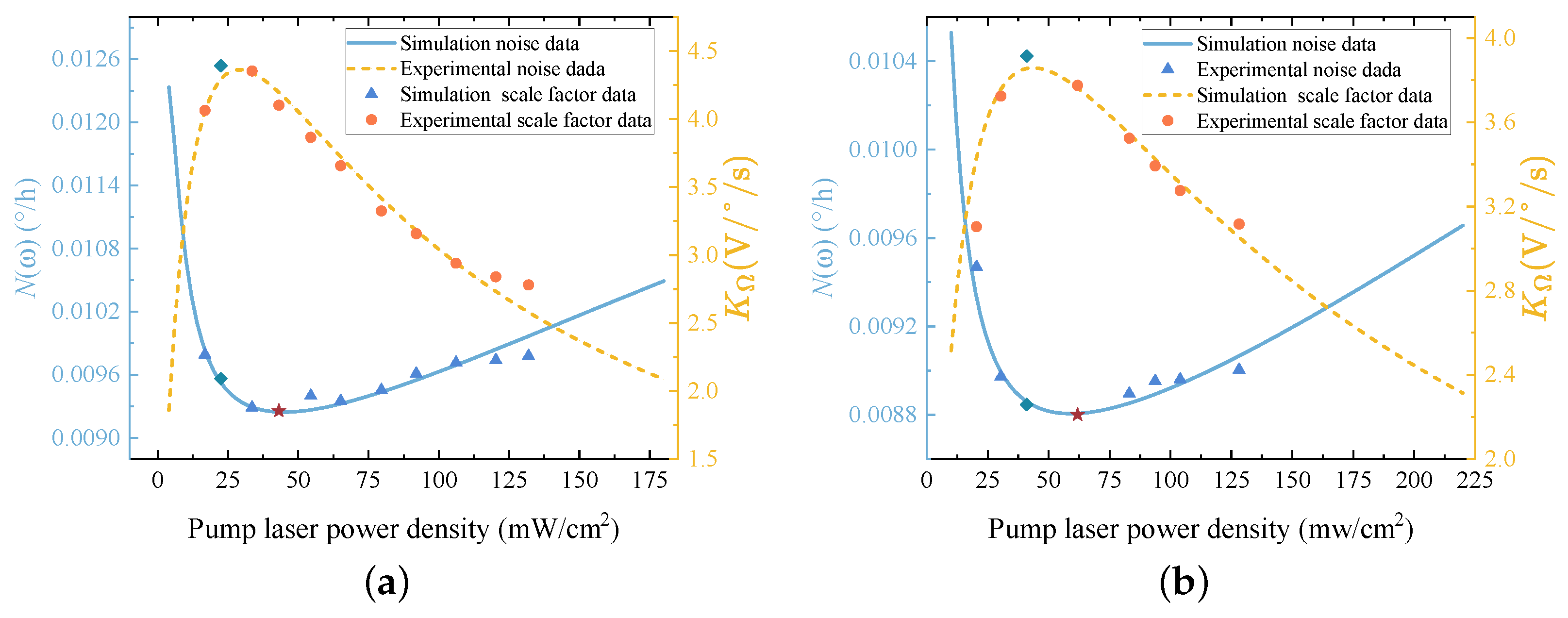
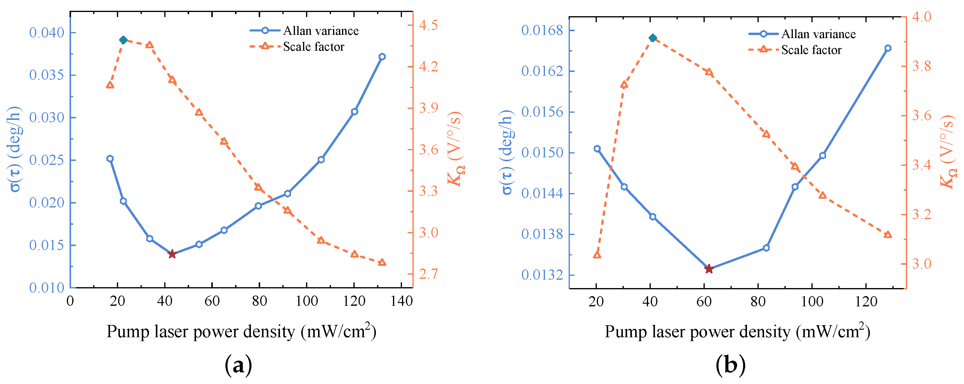
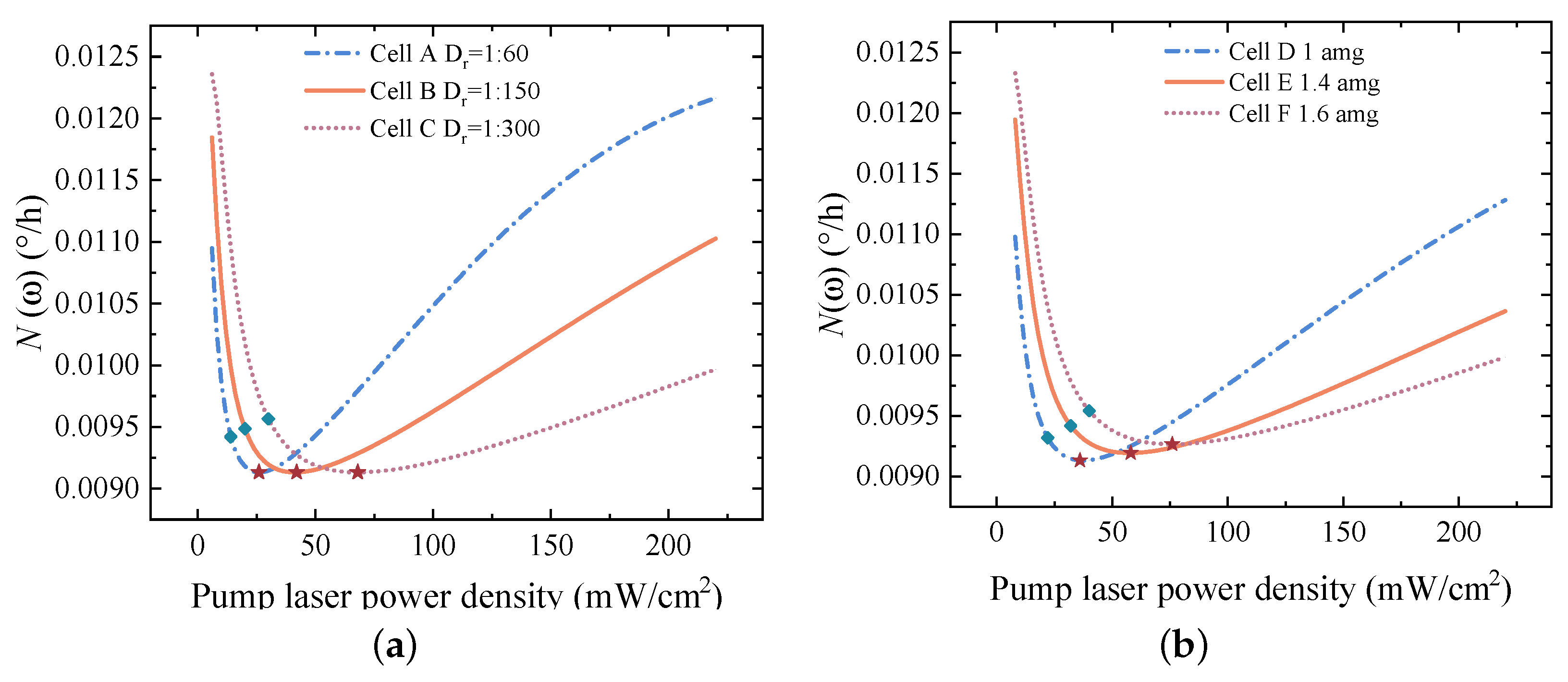
4.2. Minimum Output Noise and the Optimal Pump Laser Power Density

Substituting Equation (2) into Equation (20) and differentiating with respect to $R_p$, we obtain that when $R_p=\sqrt{R_{sd}^{e2}+R_{sd}^e{R}_{se}^{rel}}$, the scale factor $K_{\Omega }$ reaches its maximum value. The corresponding pump laser power density at this point is denoted as $L_P^{\Omega }$.

Substituting Equation (2) into Equation (26) and differentiating with respect to $R_p$, we find that the output noise $N\left(\omega \right)$ is minimized when the pumping rate

$$R_p={\left(R_{sd}^{e2}+R_{sd}^e{R}_{se}^{rel}+{\displaystyle \frac{{\gamma }^e{R}_{sd}^e{R}_2^n{C}_{mag}}{2{\omega }_n^2{N}_{bg}\left(\omega \right)}}\right)}^{1/2},$$

(27)

The pump laser power density corresponding to this rate is denoted as $L_P^{mag}$.

To calculate the output noise $N\left(\omega \right)$, the probe background noise $N_{bg}\left(\omega \right)$ and magnetic noise $\delta B_{\mathrm{mag}}\left(\omega \right)$ of the CM are tested. This can be done by applying an 8000 nT magnetic field in the direction of the pump beam and collecting output data at a sampling frequency of 200 Hz for a duration of 2 h. The Allan variance of the collected data is then calculated, and the Allan variance at $\tau =100\mathrm{s}$ is taken as $N_{bg}\left(\omega \right)$. The magnetic noise measurement involves replacing the K-Rb-²¹Ne vapor cell in the CM with a K-Rb-⁴He vapor cell and performing an FFT on the collected data. The test results show $N_{bg}\left(\omega \right)=0.0019°/\mathrm{h}$ and $\delta B_{mag}\left(\omega \right)=20\mathrm{fT}/{\mathrm{Hz}}^{-1/2}$.

In the CM, the corner frequency for hysteresis loss noise and eddy current loss noise is 5 Hz [12]. Consequently, in Equation (26) is set to 20. For practical convergence considerations, the value of $L_m$ in Equation (26) is taken as 0.001. The test results for $B_e$, $B_n$, and other parameters at different temperatures and pump laser power densities are shown in Figure 2. These data are substituted into Equation (26) to calculate the output noise $N\left(\omega \right)$ at various pump laser power densities.

The calculation results are shown as blue triangles in Figure 4. Figure 4a,b show the measurement results at 180 °C and 190 °C, respectively. The orange circles in Figure 4 represent the measured scale factor. The red pentagram marks the calculated result when $N\left(\omega \right)$ reaches its minimum value. The green diamond corresponds to the measured result when the scale factor reaches its maximum value. It can be observed that $L_P^{\mathrm{mag}}$ is greater than $L_P^{\Omega }$, and this pattern is followed at both vapor cell temperatures. The blue solid line and yellow dashed line in Figure 4 represent the simulation results based on Equations (20) and (26), respectively. The simulation results also indicate that $L_P^{mag}$ is greater than $L_P^{\Omega }$, aligning with the observed data and thus confirming our previous conclusions.

To further verify the above conclusions, we test the Allan variance under different pump laser power densities at vapor cell temperatures of 180 °C and 190 °C, as shown in Figure 5a,b, respectively. When the CM is kept stationary, the data acquisition system collects the output signal at a sampling rate of 200 Hz for a duration of 2 h. The collected data is then used to calculate the Allan variance. The values of $\sigma \left(\tau \right)$ at 100 s under different pump laser power densities are shown in Figure 5 by the diamonds. It can be seen that the pump laser power density corresponding to the minimum $\sigma \left(\tau \right)$ at 100 s (indicated by the red pentagrams) is greater than the pump laser power density at which the scale factor reaches its maximum (indicated by the green diamonds). This is consistent with our previous analysis, as the pump laser power density at which the scale factor is maximized does not correspond to the minimum system output noise. It can also be observed that the minimum $\sigma \left(\tau \right)$ at 100 s at 190 °C is lower than the minimum $\sigma \left(\tau \right)$ at 100 s at 180 °C. This is because the system output noise is lower at 190 °C.

Finally, to further validate the above conclusions and analyze the effects of the vapor cell density ratio and noble gas pressure on the CM output noise $N\left(\omega \right)$, simulations are performed for different vapor cell output noise conditions at the vapor cell temperature of 180 °C. The simulated vapor cell parameters are shown in

Table 1. Simulation parameters of vapor cell with different density ratios.

Cell Number	Density Ratio ${\mathit{D}}_{\mathit{r}}$ at 180 °C	Cell Pressure ${\mathit{p}}_{\mathbf{neon}}$ (amg)
Cell A	1:60	1
Cell B	1:150	1
Cell C	1:300	1

and

Table 2. Simulation parameters of vapor cell with different pressure.

Cell Number	Density Ratio ${\mathit{D}}_{\mathit{r}}$ at 180 °C	Cell Pressure ${\mathit{p}}_{\mathbf{neon}}$ (amg)
Cell D	1:80	1
Cell E	1:80	1.4
Cell F	1:80	1.6

. The experimental results are shown in Figure 6. From Figure 6a, it can be observed that $L_P^{mag}$ (indicated by the red pentagrams) in vapor cells with different density ratios is greater than $L_P^{\Omega }$ (indicated by the green diamonds). Moreover, as the density ratio decreases, $L_P^{mag}$ will increase. However, the minimum output noise for vapor cells with different density ratios is almost the same, which is consistent with the conclusions of previous studies [18]. For vapor cells with different pressures, $L_P^{\mathrm{mag}}$ is also greater than $L_P^{\Omega }$. Additionally, as the pressure increases, $L_P^{mag}$ also increases. Unlike the previous case, the minimum output noise of vapor cells is proportional to the pressure. The experimental results are shown in Figure 6b.

5. Conclusions

In summary, this paper systematically studies the method for determining the optimal pump laser power density in the K-Rb-²¹Ne CM while considering the effects of magnetic noise. The amplitude-frequency response and equivalent models for each frequency band are obtained through the transfer function of the CM. Based on the established model and combined with the power spectral density characteristics of magnetic noise, the noise output model is formulated. Experiments and theoretical simulations are then conducted at different vapor cell temperatures and various pump laser power densities. Both the experimental and simulation results indicate that the pump laser power density at which the output noise is minimized is greater than that at which the scale factor is maximized. Moreover, at the pump laser power density corresponding to the minimum output noise, the output noise can be reduced by approximately 25%. And the Allan variance at 180 °C and 190 °C are 0.01395°/h and 0.01329°/h, respectively. Finally, the variation patterns of the optimal pump laser density point and the minimum output noise under different density ratios and pressure are simulated. The simulation results indicate that although the optimal pump laser power density varies for vapor cells with different density ratios, the minimum output noise remains almost consistent. For vapor cells with different pressures, as the pressure increases, the optimal pump laser power density gradually increases, and the minimum output noise also rises. The theories and methods proposed in this paper provide significant reference value for selecting the optimal pump laser power density and suppressing magnetic noise in co-magnetometers. However, this study has overlooked the impact of random white noise in the system, and thus further research in this area is necessary.

References

1. Flambaum, V.V.; Romalis, M.V. Limits on Lorentz Invariance Violation from Coulomb Interactions in Nuclei and Atoms. Phys. Rev. Lett. 2017, 118, 142501.1–142501.4. [Google Scholar] [CrossRef] [PubMed]
2. Terrano, W.A.; Romalis, M.V. Comagnetometer probes of dark matter and new physics. Quantum Sci. Technol. 2021, 7, 014001. [Google Scholar]
3. Wang, Z.; Peng, X.; Zhang, R.; Luo, H.; Guo, H. Single-Species Atomic Comagnetometer Based on 87Rb Atoms. Phys. Rev. Lett. 2020, 124, 193002. [Google Scholar] [CrossRef]
4. Wei, K.; Ji, W.; Fu, C.; Wickenbrock, A.; Flambaum, V.V.; Fang, J.; Budker, D. Constraints on exotic spin-velocity-dependent interactions. Nat. Commun. 2022, 13, 7387. [Google Scholar] [CrossRef] [PubMed]
5. Shi, M. Investigation on magnetic field response of a 87Rb- 129Xe atomic spin comagnetometer. Opt. Express 2020, 28, 32033. [Google Scholar] [CrossRef]
6. Pei, H.; Duan, L.; Ma, L.; Fan, S.; Cai, Z.; Wu, Z.; Fan, W.; Quan, W. Real-time quantum control of spin-coupling damping and application in atomic spin gyroscopes. Cell Rep. Phys. Sci. 2024, 5, 101832. [Google Scholar] [CrossRef]
7. Kornack, T.W.; Ghosh, R.K.; Romalis, M.V. Nuclear Spin Gyroscope Based on an Atomic Comagnetometer. Phys. Rev. Lett. 2005, 95, 230801. [Google Scholar] [CrossRef]
8. Fang, J.; Wan, S.; Yuan, H. Dynamics of an all-optical atomic spin gyroscope. Appl. Opt. 2013, 52, 7220–7227. [Google Scholar] [CrossRef]
9. Ledbetter, M.P.; Savukov, I.M.; Acosta, V.M.; Budker, D.; Romalis, M.V. Spin-exchange relaxation free magnetometry with Cs vapor. Phys. Rev. 2007, 77, 1012–1015. [Google Scholar] [CrossRef]
10. Fang, J.; Chen, Y.; Zou, S.; Liu, X.; Hu, Z.; Quan, W.; Yuan, H.; Ding, M. Low frequency magnetic field suppression in an atomic spin co-magnetometer with a large electron magnetic field. J. Phys. B At. Mol. Opt. Phys. 2016, 49, 065006. [Google Scholar] [CrossRef]
11. Chen, Y.; Quan, W.; Duan, L.; Lu, Y.; Jiang, L.; Fang, J. Spin-exchange collision mixing of the K and Rb ac Stark shifts. Phys. Rev. A 2016, 94, 052705. [Google Scholar] [CrossRef]
12. Fan, W.; Quan, W.; Liu, F.; Pang, H.; Xing, L.; Liu, G. Performance of Low-Noise Ferrite Shield in a K-Rb-21Ne Co-Magnetometer. IEEE Sens. J. 2020, 20, 2543–2549. [Google Scholar] [CrossRef]
13. Li, R.; Quan, W.; Fan, W.; Xing, L.; Fang, J. Influence of magnetic fields on the bias stability of atomic gyroscope operated in spin-exchange relaxation-free regime. Sens. Actuators A Phys. 2017, 266, 130–134. [Google Scholar] [CrossRef]
14. Fu, Y.; Fan, W.; Ruan, J.; Liu, Y.; Lu, Z.; Quan, W. Effects of Probe Laser Intensity on Co-Magnetometer Operated in Spin-Exchange Relaxation-Free Regime. IEEE Trans. Instrum. Meas. 2022, 71, 9501607. [Google Scholar] [CrossRef]
15. Jiang, L.; Quan, W.; Liang, Y.; Liu, J.; Duan, L.; Fang, J. Effects of pump laser power density on the hybrid optically pumped comagnetometer for rotation sensing. Opt. Express 2019, 27, 27420–27430. [Google Scholar] [CrossRef]
16. Zhao, T.; Zhai, Y.; Liu, C.; Xie, H.; Cao, Q.; Fang, X. Spin polarization characteristics of hybrid optically pumped comagnetometers with different density ratios. Opt. Express 2022, 30, 28067–28078. [Google Scholar] [CrossRef]
17. Liu, Y.; Fan, W.; Fu, Y.; Pang, H.; Pei, H.; Quan, W. Suppression of Low-Frequency Magnetic Drift Based on Magnetic Field Sensitivity in K-Rb-21Ne Atomic Spin Comagnetometer. IEEE Trans. Instrum. Meas. 2022, 71, 13361–13371. [Google Scholar] [CrossRef]
18. Fu, Y.; Fan, W.; Ruan, J.; Liu, Y.; Wang, Z.; Zhou, X.; Quan, W. Analysis on the effect of electron spin polarization on a hybrid optically pumped K-Rb-21Ne co-magnetometer. Opt. Express 2022, 30, 42114–42128. [Google Scholar] [CrossRef]
19. Fan, W.; Quan, W.; Liu, F.; Xing, L.; Liu, G. Suppression of the Bias Error Induced by Magnetic Noise in a Spin-Exchange Relaxation-Free Gyroscope. IEEE Sens. J. 2019, 19, 9712–9721. [Google Scholar] [CrossRef]
20. Wu, Z.; Pang, H.; Wang, Z.; Fan, W.; Liu, F.; Liu, Y.; Quan, W. A New Design Method for a Triaxial Magnetic Field Gradient Compensation System Based on Ferromagnetic Boundary. IEEE Trans. Ind. Electron. 2024, 71, 13361–13371. [Google Scholar] [CrossRef]
21. Kornack, T.W.; Romalis, M.V. Dynamics of two overlapping spin ensembles interacting by spin exchange—Art. no. 253002. Phys. Rev. Lett. 2002, 89, 253002. [Google Scholar] [CrossRef]
22. Wei, K.; Zhao, T.; Fang, X.; Li, H.; Quan, W. Simultaneous Determination of the Spin Polarizations of Noble-Gas and Alkali-Metal Atoms Based on the Dynamics of the Spin Ensembles. Phys. Rev. Appl. 2020, 13, 044027. [Google Scholar] [CrossRef]
23. Cates, G.D.; Schaefer, S.R.; Happer, W. Relaxation of spins due to field inhomogeneities in gaseous samples at low magnetic fields and low pressures. Phys. Rev. A 1988, 37, 2877. [Google Scholar] [CrossRef]
24. Romalis, M.V.; Cates, G.D. Accurate 3He polarimetry using the Rb Zeeman frequency shift due to the Rb-3He spin-exchange collisions. Phys. Rev. A 1998, 58, 3004. [Google Scholar] [CrossRef]
25. Romalis, M.V. Hybrid Optical Pumping of Optically Dense Alkali-Metal Vapor without Quenching Gas. Phys. Rev. Lett. 2010, 105, 243001. [Google Scholar] [CrossRef]
26. Fan, W.; Quan, W.; Zhang, W.; Xing, L.; Liu, G. Analysis on the Magnetic Field Response for Nuclear Spin Co-Magnetometer Operated in Spin-Exchange Relaxation-Free Regime. IEEE Access 2019, 7, 28574–28580. [Google Scholar] [CrossRef]
27. Fu, Y.; Sun, J.; Ruan, J.; Quan, W. A nanocrystalline shield for high precision co-magnetometer operated in spin-exchange relaxation-free regime. Sens. Actuators A Phys. 2022, 339, 113487. [Google Scholar] [CrossRef]
28. Pei, H.; Yu, W.; Fan, W.; Du, P.; Quan, W. Bandwidth Expansion of Atomic Spin Gyroscope With Transient Response. IEEE Trans. Instrum. Meas. 2022, 71, 1502308. [Google Scholar] [CrossRef]
29. Xu, Z.; Wei, K.; Zhao, T.; Cao, Q.; Liu, Y.; Hu, D.; Zhai, Y. Fast Dynamic Frequency Response-Based Multiparameter Measurement in Spin-Exchange Relaxation-Free Comagnetometers. IEEE Trans. Instrum. Meas. 2021, 70, 7007110. [Google Scholar] [CrossRef]
30. Lu, Y.; Zhai, Y.; Fan, W.; Zhang, Y.; Xing, L.; Jiang, L.; Quan, W. Nuclear magnetic field measurement of the spin-exchange optically pumped noble gas in a self-compensated atomic comagnetometer. Opt. Express 2020, 28, 17683–17696. [Google Scholar] [CrossRef]
31. Liu, J.; Jiang, L.; Liang, Y.; Liu, F.; Quan, W. A Fast Measurement for Relaxation Rates and Fermi-Contact Fields in Spin-Exchange Relaxation-Free Comagnetometers. IEEE Trans. Instrum. Meas. 2020, 69, 7805–7812. [Google Scholar] [CrossRef]
32. Yuan, L.; Huang, J.; Fan, W.; Wang, Z.; Zhang, K.; Pei, H.; Cai, Z.; Gao, H.; Liu, S.; Quan, W. Measurement and analysis of polarization gradient relaxation in the atomic comagnetometer. Measurement 2023, 217, 113043. [Google Scholar] [CrossRef]
Figure 1. Experimental setup of the SERF CM. PSS, power stabilization system. PD, photodiode. LCVR, liquid-crystal variable retarder. PBS, polarizing beam splitter. GT, Glan-Taylor polarizer. λ / 2 , half wave plate. λ / 4 , quarter-wave plate.
Photonics 11 00835 g001
Figure 2. The parameter measurement results of the CM under different pump laser power densities are as follows. (a) shows B e and B n at different pump laser power densities. And circular and diamond markers represent the measured data, while solid and dotted lines denote the fitted curves. (b) shows R 2 e and R 2 n at different pump laser power densities.
Photonics 11 00835 g002
Figure 3. Verification of the equivalent models for each frequency band is shown. The orange diamonds and purple circles represent the measured data points, while the green and blue lines represent the equivalent models for each frequency band calculated from the parameters. Different line styles are used to distinguish between the frequency bands.
Photonics 11 00835 g003
Figure 4. System output noise N ( ω ) and scale factor K Ω under different pump laser power densities. (a) At 180 °C, the variation of N ( ω ) and K Ω under different pump laser power densities. The orange circles represent the measured values of K Ω , and the yellow dashed line represents the simulated values of K Ω . The blue triangles represent the calculated values of the output noise N ( ω ) , and the blue solid line represents the simulated values of N ( ω ) . The red pentagrams indicate the minimum output noise, and the green diamonds indicate the maximum scale factor. (b) At 190 °C, the variation of N ( ω ) and K Ω under different pump laser power densities.
Photonics 11 00835 g004
Figure 5. Allan variance at 100s and scale factor test results under different pump laser power densities. (a) Variation of K Ω and σ ( τ ) at 100 s under different pump laser power densities at the vapor cell temperature of 180 °C. The red pentagrams indicate the minimum σ ( τ ) at 100 s, and the green diamonds mark the maximum K Ω . (b) Variation of K Ω and σ ( τ ) at 100 s under different pump laser power densities at the vapor cell temperature of 190 °C.
Photonics 11 00835 g005
Figure 6. Simulation results of the optimal pump laser power density and the minimum output noise for different density ratios and different gas pressures. (a) shows the simulation results for a vapor cell temperature of 180 °C and different density ratios. The red pentagram marks the point of minimum output noise, and the green diamond corresponds to the point of maximum scale factor. (b) shows the simulation results for a vapor cell temperature of 180 °C and different pressures.
Photonics 11 00835 g006