Abstract
Free-space optical communications have emerged as a powerful solution for inter-satellite links, playing a crucial role in next-generation satellite networks. This paper introduces a comprehensive model that enables the dynamic evaluation of optical power requirements for realistic low Earth orbit satellite constellations throughout the orbital period. Our approach incorporates the constellation architecture, link budget analysis, and optical transceiver design to accurately estimate the power required for sustaining connectivity for both intra- and inter-orbit links. We apply the model considering Walker delta-type constellations of varying densities. We show that in dense constellations, even at high data rates, the required transmission power can be low enough to mitigate the need for optical amplification. Dynamically estimating the power requirements is vital when evaluating energy savings in adaptive scenarios where terminals adaptively change the emitted power depending on the link status. Our model is implemented in Python and is openly available under an open-source license. It can be easily adapted to various alternative constellation configurations.
1. Introduction
In recent decades, there has been a notable surge in free-space optics (FSO) driven by the escalating demand for real-time quality of service and the necessity to efficiently transfer large amounts of data both at terrestrial and satellite networks, with a pronounced focus on optical inter-satellite links (OILs) [1]. While radio-frequency (RF) technologies are still prominent in satellite applications, the emergence of OILs is quickly gaining leverage in commercial applications. OILs offer several key advantages, including a vast available spectrum, high data rates, narrow optical beams favoring security, small antenna sizes, and reduced power consumption [2,3,4,5].
Low Earth orbit (LEO) Walker-delta type constellations are widely being considered in commercial deployments, with Starlink Phase 1 V2 being a typical example [6,7]. This constellation consists of a total of 1584 mini-satellites at an altitude of 550 km. In LEO applications, satellite sizes vary from large to pico satellites, the latter commonly being referred to as cubesats [8]. OILs are a favorable communication solution in all these scenarios, leading to laser terminals that are both lightweight and compact [9].
Various OIL systems have been developed. One notable example is the Optel- terminal, constructed by TNO and utilized for both downlink and uplink communications [10]. Another is the LCT terminal produced by TESAT, which is employed for LEO satellite networks [11]. NASA has also developed several systems for LEO-to-LEO and LEO-to-ground communication links [12]. Similarly, the German Aerospace Center has also demonstrated mini-satellite OIL transceivers [13]. In [14], a spherical system with multiple transceivers was developed, which offers omnidirectional coverage of nearly 360 degrees and a data rate of 1 Gbps over a distance of 200 km. Another approach, as described in [15], involves equipping each satellite side with a 100-degree field-of-view OIL, which also enables omnidirectional coverage.
Motivation and Related Work
Understanding the system requirements to maintain connectivity throughout a constellation is crucial. Several studies have examined the structure of satellite constellations and communications between different satellite layers. In [16], a classification of both RF and OIL links is presented, focusing on links between satellites at the same or different altitudes and between high-altitude platforms (HAPs). In [17], a satellite network utilizing OILs is examined and compared to a terrestrial network in terms of latency. In [18], the phasing parameter F is introduced to determine the relative initial satellite positions to avoid collisions. In [19,20], OIL connection strategies are explored, focusing on efficient routing schemes with low latencies. In [20], the authors introduced a latitude parameter to examine the relationship between satellite distance and the number of connections that could be established. The authors in [6] focused on the trade-off between physical layer parameters and network latencies in intercontinental satellite links. In [21], a methodology is proposed to minimize the average network latency in intercontinental connections. In [22], the authors proposed a methodology for utilizing OILs to reduce latencies and determine the most efficient routing. In [23], the impact of atmospheric effects on optical space communications—such as signal attenuation and scintillation—is analyzed, along with their potential utilization for atmospheric measurements. The work also explores the adaptability of laser communication terminals and highlights the synergy between satellite technologies and atmospheric research. However, such factors are not considered in the present study.
The primary contribution of this work is the application of a comprehensive network model to analyze optical power requirements at OIL terminals in LEO Walker delta-type constellations [24] that are widely being considered in commercial applications. The required optical power is a crucial factor that directly affects terminal design, influencing transmitter and receiver specifications, power acquisition and tracking system precision, thermal management strategies, and overall power consumption. Previous studies have typically considered the link budget without (a) accounting for the precise constellation dynamics and (b) the actual network requirements for connectivity, which involves reliable intra- and inter-orbit communication. Our approach incorporates the full constellation dynamics and is applicable to commercial constellations such as Kuiper and Starlink [6,18]. We use the Starlink Phase 1 V2 constellation as a realistic scenario to illustrate the practical applicability of our model. We applied it in two different scenarios with varying satellite densities and estimated the power requirements for high-speed optical inter-satellite links (OILs). Our results are comparable to [19,20] in terms of minimum distances between satellites and indicate that a 100 Gbps network can be sustained across a dense constellation of approximately 6000 satellites using transmission powers in the 300 mW range. This is an important finding, since such power levels can be supported by high-power distributed feedback (DFB) lasers [25], possibly removing the need for optical amplification, simplifying the terminal design and reducing power consumption. Such levels of satellite population are well within the planning of commercial satellite internet carriers [22,26].
Our comprehensive model is implemented as a Python module that encompasses various constellation parameters, such as satellite count, initial positioning, inclination, and phasing, as well as terminal characteristics, including beam divergence, targeted bit error rate (BER), receiver aperture, etc., to precisely calculate physical layer performance. Also, in a straightforward way, it optimizes satellite phasing in a standard manner following [4,18]. Our results indicate that the required optical power can vary significantly over an orbital period in links between satellites in adjacent orbits. These calculations are useful in evaluating adaptive optical satellite network strategies, where link parameters such as the transmission power are dynamically adjusted. Such adaptive approaches can lead to significant savings in energy consumption, minimize thermal stress, and potentially prolong the operational lifetime [27]. The model’s source code is publicly available [28] on the web to foster collaboration and facilitate the utilization of our research outcomes within the scientific community. The model is easily extendable to a wide selection of constellation types, modulation formats, and detection schemes.
The rest of the paper is organized as follows: in Section 2, we start by outlining how to account for constellation dynamics. In addition, we discuss how the initial satellite position can be optimized in order to minimize the chance of collisions. We also outline the satellite connectivity requirements assumed in our work. Section 3 describes the link budget model adopted to estimate physical layer performance. We discuss channel gain and how beam divergence can be optimized in the presence of pointing errors. We also calculate the noise power estimation, the bit error rate (BER), and the receiver sensitivity. Appendix A discusses some implementation details of the Python module. Section 4 presents the results obtained from our model, emphasizing the estimated power requirements for various constellation architectures. Some concluding remarks are given in Section 5.
2. Constellation Model
2.1. Constellation Dynamics
The equations describing the motion of the satellite with a circular orbit can be derived using the general approach of [29]. In three-dimensional space, the satellite’s position relative to the Earth’s center is described by a three-component vector , with denoting the vector’s transpose. Figure 1 shows an Earth-centered coordinate system where the plane contains the equatorial plane (orange dashed line), while the z-axis aligns with the Earth’s rotation axis, pointing north. The figure illustrates the basic parameters involved in estimating the satellite position. In the figure, denotes the distance of the satellite from the Earth’s center. In this paper, we study circular orbits, and hence, r remains constant.
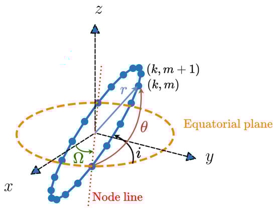
Figure 1.
Satellite frame of reference and various orbital parameters used to determine the orbital dynamics.
Assuming a constellation consisting of orbits containing satellites each. Every satellite can be identified by the index k of its orbit and its index m within the orbit. Its position is determined by [29]
where
is the position of the satellite with respect to the perifocal frame of reference (i.e., the frame attached to the satellite itself), i is the inclination angle, and is the angle between the x-axis and the node line for orbit k determined by
while h is the magnitude of the angular momentum related to the satellite’s period T through . The period of the circular orbit is given by
with being the product of the gravitational constant, , and the mass of the earth, . The transformation matrix in (1) is given by
The true anomalies in circular orbits are determined by
We can assume that on each orbit k, the satellites are evenly spaced, in which case
where is the initial anomaly of the first satellite at the orbit. Given these initial anomalies, we can combine (6) and (7) to obtain the values of for every time instance t and calculate the position of every satellite in the constellation using (1)–(5).
Table 1 presents the constellation parameters representative of Starlink’s Phase 1 V2, which, unless otherwise specified, serves as a reference in our simulations. Figure 2 illustrates the satellite trajectories for this constellation. Due to the inclination of the constellation, the satellite trajectories are more widely spaced near the equator and progressively converge as they approach higher latitudes. Beyond a certain latitude near the poles, satellite coverage diminishes entirely.

Table 1.
Orbital parameters.
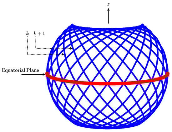
Figure 2.
Satellite trajectories (colored in blue) for the Walker-delta constellation of Table 1. The equator is shown in red.
2.2. Collision Avoidance
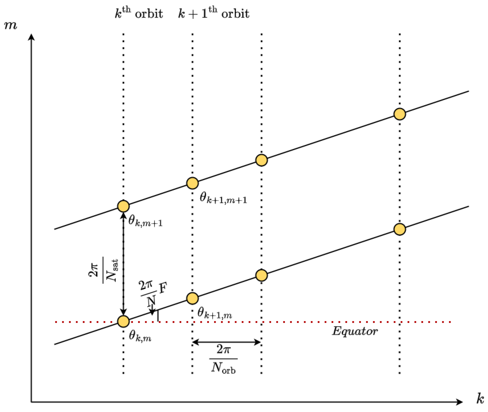
To avoid collisions within the constellation, we adopt the approach of [18]. For each orbit k, we assume that the satellites are placed so that
where N is the total number of satellites in the constellation . The parameter F is an integer in the range of . This scheme is illustrated in Figure 3.

Figure 3.
Illustration of the relationship between the true anomalies of the satellites at the same and adjacent orbits, the phasing factor F, and the number of orbits and satellites per orbit, and , respectively, on the Equatorial Plane.
To choose the optimal value for F, we can run simulations considering various possible values of F to determine the minimum satellite-to-satellite distance over an orbital period, . We can significantly speed up the computations by leveraging the uniformity of the constellation. Thus, instead of considering all possible combinations of satellites, we can focus on one particular satellite and calculate the distances to all other satellites within one orbital period [19,20].
The optimal value of F, as determined in our model (Table 1), was calculated using the Pyminisat module (as referenced in Appendix A) considering [6] and selected for the remaining simulations of this constellation.
2.3. Connectivity Requirements
We now discuss the requirements that need to be imposed to guarantee network connectivity throughout the constellation. This typically involves conditions imposed on both intra- and inter-orbit links. Figure 4 illustrates a typical scenario where a reference satellite communicates with its adjacent satellites. The satellites and are the two nearest satellites in the same orbit k as . The satellites , , and are the first, second, and third closest satellites to , respectively, located at the next orbit, . Similarly, , , and are the first, second, and third closest satellites to , respectively, located in the previous orbit, . This group of satellites forms a swarm of nine satellites around with a constant line of sight. We assume that the connectivity of with the rest of the satellites of is the minimum requirement to achieve reliable communication with the rest of the network, providing various alternative paths for data routing. This must be met for the swarm of every satellite in the constellation, as it implies that any two satellites in the communication can communicate with each other using a single hop or multiple hops. Similar to what we discuss in Section 2.2, due to the uniformity of the constellation, it is not necessary to address the swarms formed around every satellite in the constellation. Instead, we can focus on just a single reference satellite, since the distance variation between satellites in the swarm will be the same if we change the reference satellite , albeit with a time offset.
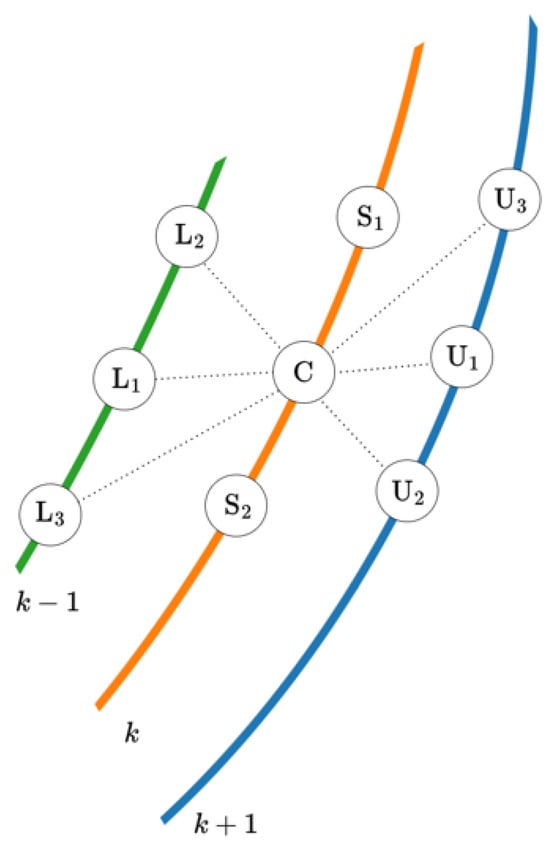
Figure 4.
The satellite connectivity requirements considered in this work. Each satellite must, at all times, communicate which its two closest neighbors in the same orbit ( and ) as well as its three nearest satellites in the lower orbit and upper orbit, respectively.
Since satellites in the same orbit move at a constant angular velocity, the distance between and and will be constant with t. This is not true for the distances between and or due to the difference in the angles . As mentioned in Section 2.2, we introduce a relative initial anomaly difference between orbits. The first orbit begins from the Earth’s equatorial frame with a latitude of . The next orbit shifts in longitude by an amount equal to , and so on. However, the closest neighboring satellites in the adjacent upper or lower orbits remain fixed relative to any satellite within the same orbit: the nearest upper-orbit neighbor, , maintains its position relative to throughout ’s orbital period, and this pattern holds for other inter-orbit neighbors as well. At time , we can calculate the distances from to all satellites in adjacent orbits and identify the three nearest satellites in each orbit to determine the swarm .
3. Link Model
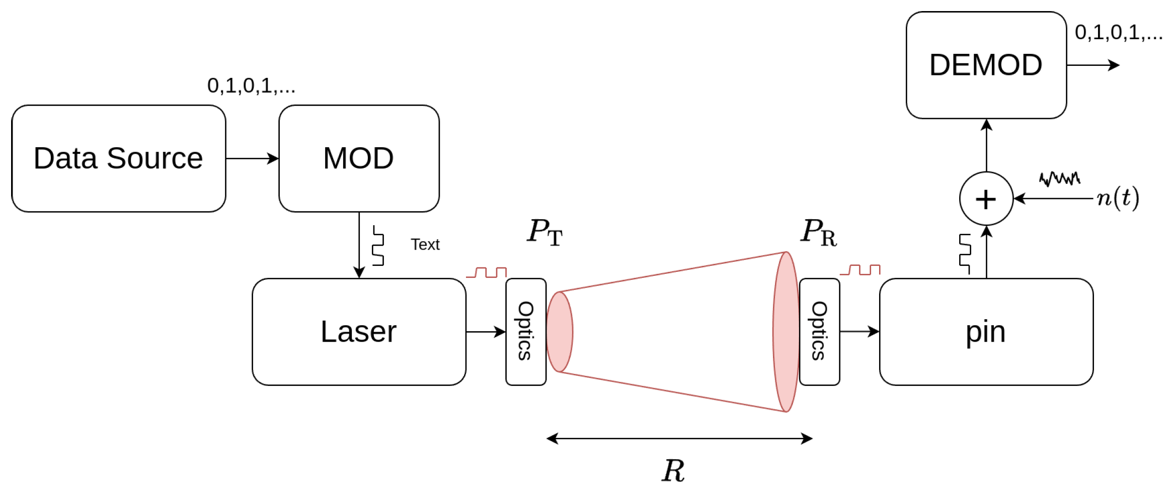
In this section, we elaborate on the link model adopted in order to calculate the physical layer performance and the required optical transmitter power to maintain connectivity. Figure 5 shows the basic block diagram of an OIL. The data source modulates the amplitude produced by a laser diode, and after the beam is shaped by the transmitter optics, it propagates in free space until it reaches the receiving end where a receiver converts the incoming light back to an electrical signal. The performance is impaired by the additive white Gaussian noise (AWGN) added to the signal. In what follows, we assume an intensity modulation/direct detection (IM/DD) with on–off keying (OOK) and note that the model could be extended to also account for multi-level schemes [30], polarization [31] or wavelength division multiplexing [32], and coherent detection [33].

Figure 5.
Block diagram of the OIL model, consisting of the data source, the modulator (MOD), the laser transmitter, the transmitter optics, the optical channel, the receiver optics and photodiode (pin), and the demodulator (DEMOD).
3.1. Link Budget
Given the satellite positions at any time t, we can use a link budget model to dynamically estimate the minimum transmitted power required to maintain link connectivity over an entire orbital period T. Assuming any two satellites described by the pairs of integers and , their distance is simply determined as
In free space, the link budget equation relating the received power and the transmitted power can be written as [5]
where
is the channel gain, and are the standard deviations of the pointing errors at the transmitter and receiver sides, respectively; and are the optical efficiency of the transmitter and receiver, respectively; while and are the transmitter and receiver gains determined by
where is the divergence of the transmitting beam, is the receiver’s telescope diameter, and is the wavelength. The required received power is determined by the receiver sensitivity and the required link margin as follows [5]:
We discuss the estimation of the receiver sensitivity in the next subsections. There is an optimal value for lying in between that can be found by maximizing (11). Taking the first derivative of with respect to , we readily see that the optimal beam divergence is
We, therefore, consider this beam divergence value in our calculations.
3.2. Bit Error Rate
The bit error rate (BER), , in the case of OOK is given as [34]
where Q is the Q-function, and its argument is determined by
In (18), denotes the average optical received power, , where and are the optical received powers corresponding to bit and , respectively. Additionally, denotes the extinction ratio, and represents the responsivity,
where is the electron charge, is Planck’s constant, is the internal quantum efficiency, and is the optical frequency, with c being the speed of light in vacuum and and the corresponding noise standard deviations, determined by
where represents the shot noise for or obtained by replacing with and , respectively. In this equation, is the electrical bandwidth, which is related to the data rate by , where is the roll-off factor, assumed to be zero in this study, and is the thermal noise power, given by [34]
In (22), is Boltzmann’s constant, the temperature measured in Kelvin (), is the receiver amplifier noise figure, and the load resistance.
3.3. Receiver Sensitivity
Given the required BER , we can estimate the receiver sensitivity as the average power required by first inverting (17) to obtain the required value of . The inverse of the Q function can be written in terms of the inverse of the error function , which can be estimated through standard Python libraries:
Once the target value of is obtained through (23), we can substitute Equations (21) and (20) in (18) to obtain the following solution for the required receiver sensitivity :
where
Equations (24) and (25) can be used to determine the receiver sensitivity given the receiver parameters. One can then determine the required received power using (15) and then estimate the required transmitter power using (11). It is critical to note that these sensitivity values assume ideal synchronization conditions. In practice, timing recovery (e.g., Gardner loops) and adaptive equalization [35] are mandatory to mitigate BER degradation from LEO-specific impairments.
In our calculations, we deal with the uncoded BER and do not account for forward error correction (FEC). FEC may enhance the system’s BER performance once the uncoded BER exceeds a given threshold value . Hence, we may set the target BER in (17) equal to to obtain the required optical power. In addition, we do not account for signal processing algorithms that can enhance the BER performance [35]. This is because for the constellation altitudes and inter-satellite link distances considered, the optical channel is approximately flat.
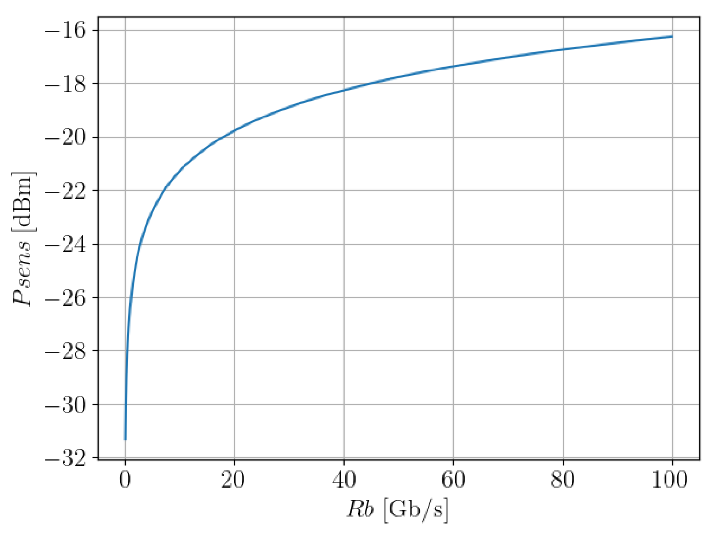
In Figure 6, we illustrate the values obtained for , assuming the parameters in Table 2. As expected, the sensitivity value increases with the data rate reaching just below ≅ at .

Figure 6.
Receiver sensitivity with respect to the data rate obtained for the parameters of Table 2.
Table 2.
System parameters.
The various model elements discussed in Section 2 and Section 3 were implemented as part of the Pyminisat Python module [28], which is publicly available under an open-source license. Details about the inner workings and the model implementation can be found in Appendix A. The model’s Github repository further describes how the initialization parameter can be adapted to the constellation at hand.
4. Results
In this section, we apply the Pyminisat module to study the constellation dynamics and power requirements for the system parameters summarized in Table 1 and Table 2, which we refer to as Scenario A. It is interesting to point out that data rates assumed in Table 2 are in accordance with existing terminal technologies [19,36]. Pointing error levels are indicative of values reported in the literature [37,38]. A value of is assumed for the extinction ratio, which is typical of commercially available lithium niobate electro-optic modulators. In addition, the choice of the receiver telescope diameter and wavelength is also compatible with state-of-the-art optical terminal specifications [1].
We also consider two alternative scenarios: Scenario B, where the number of satellites per orbit and the number of orbits are reduced by half, resulting in a thinner constellation with the total number of satellites N compared to Scenario A. In Scenario C, and are doubled compared to Scenario A, resulting in a quadrupled N, and hence, we obtain a denser constellation. The constellations remain uniform in all scenarios. Note that the total number of satellites N in Scenario C remains well within the planning of commercial satellite internet constellation deployments [22,26].
Table 3 summarizes key properties of the constellations for the three scenarios considered, derived using the Pyminisat module, as referenced in Appendix A. For all scenarios, we assume an inclination angle i equal to and an altitude of Km. The table quotes the optimal F obtained for each constellation, the inter-satellite distance between two consecutive satellites in the same orbit, as well as the maximum and minimum link distances required ( and , respectively) to achieve network connectivity, considering the links to adjacent satellites as outlined in Section 2.3.
Table 3.
Scenarios considered.
4.1. Scenario A
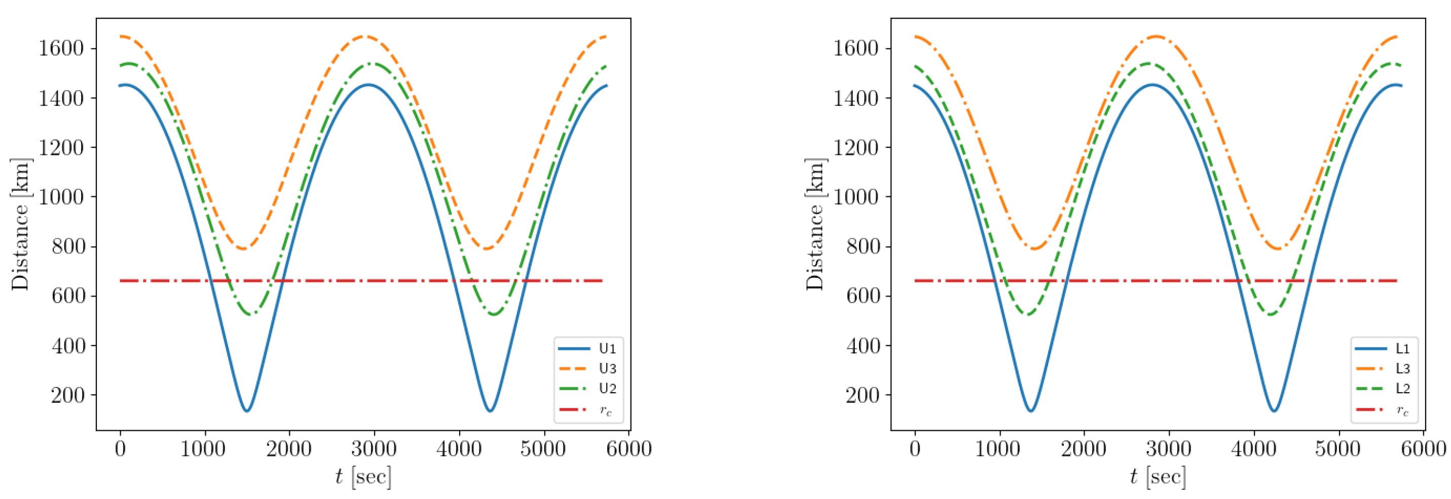
Scenario A is similar to Starlink’s Phase 1 V2 constellation [6]. The optimal F is equal to 13 as quoted in Table 3. To ensure connectivity across the network as discussed in Section 2.3, we first need to estimate the distances between a satellite and its adjacent neighbors. Figure 7 (left, right) show the distances of the upper- and lower-orbit adjacent satellites for satellite . For this constellation, the distance between two consecutive satellites in the same orbit is km. We observe that, in both cases, the distances between the satellite and its upper- and lower-orbit neighbors fluctuate significantly within one orbital period, ranging from km to km. These distance fluctuations exhibit a periodic behavior as the central satellite moves through the upper and lower halves of its trajectory around the Earth. Due to the uniformity of the constellation, these fluctuations are practically the same for the upper- and lower-orbit neighbors, and , respectively, differing only by an initial time displacement. The figures indicate the varying conditions for inter-orbit links: while intra-orbit link distances remain constant at , the inter-orbit link length varies from about one fifth of to more than twice that.
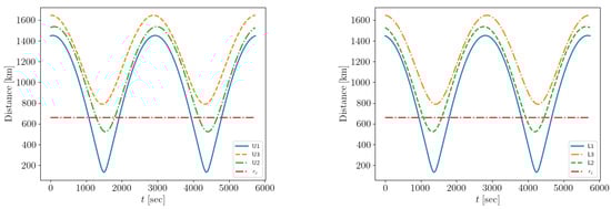
Figure 7.
Distance variations between satellite and its adjacent neighbors: (left) in the upper orbit and (right) in the lower orbit, observed over one orbital period. The intra-orbit link length between consecutive satellites remains constant throughout.
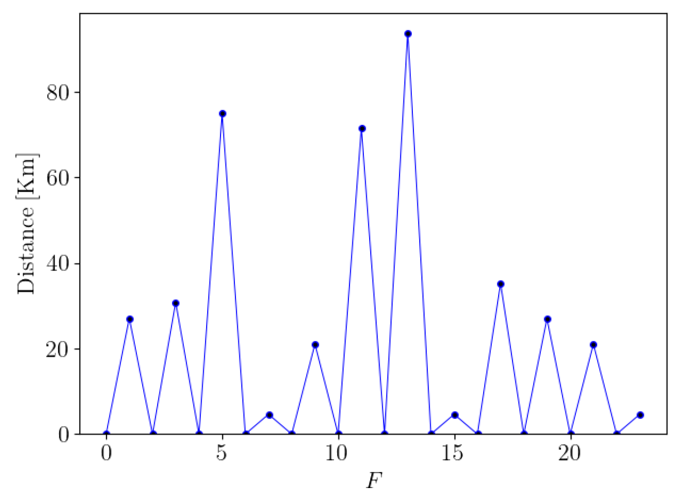
As mentioned in Section 2.2, the F value is used to determine the allocation of satellites within a constellation, ensuring a minimum safe distance between them. To achieve the safest possible configuration, we analyze how the minimum distance varies with changes in the F value, as illustrated in Figure 8. Using the Constellation class from Pyminisat, as referenced in Appendix A, we incorporate constellation dynamics to determine the optimal F value. The optimal F value is the one that maximizes the minimum distance between satellites, ensuring the most efficient and secure allocation.
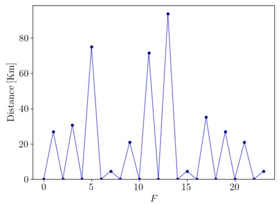
Figure 8.
Minimum distance between satellites in the constellation relative to changes in the F value for Scenario A. We chose an F value of 13 to maximize the safe distance between satellites.
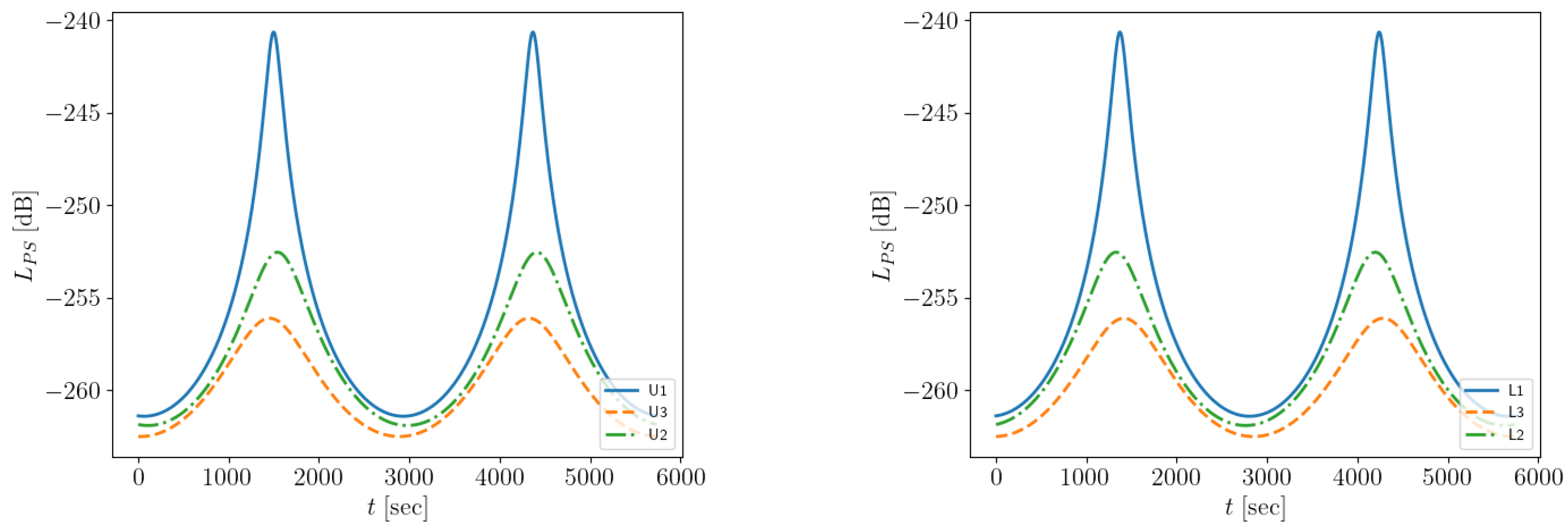
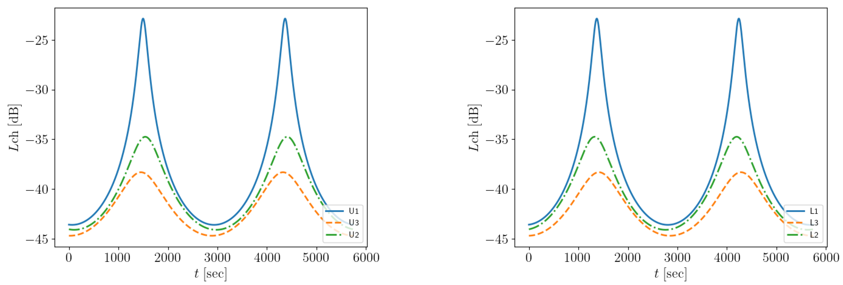
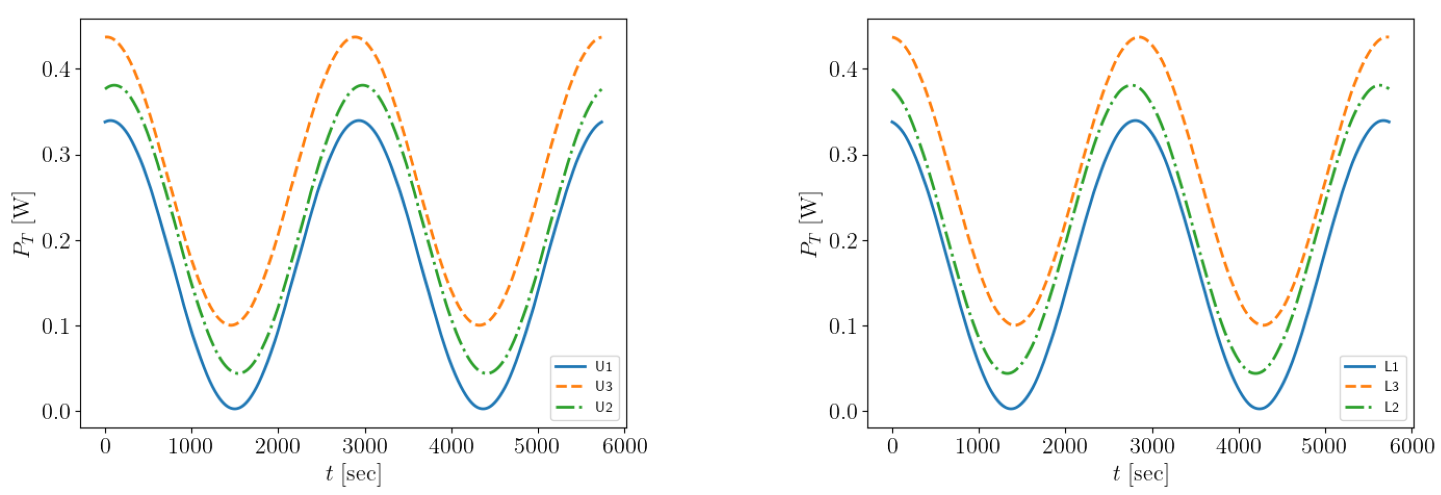
In Figure 9 and Figure 10, we show the variations in path loss and channel gain , respectively, for the links between the central satellite and both the upper- and lower-orbit neighbors. Both and follow an inverse square variation (∝ with respect to the corresponding inter-satellite distance R. For the set of parameters in Table 1 and Table 2, the transmitter and receiver gains are = 120 dB and = 104.2 dB, respectively, while the transmitter and receiver pointing losses are = −4.3 dB and = −0.11 dB, respectively. High transmitter and receiver gains are necessary to compensate for the path losses shown in Figure 9. This is a clear advantage of optical inter-satellite links (OILs), which can utilize highly collimated beams to optimize the link budget. Next, we discuss the transmitter power required to maintain the links between all adjacent satellites of Figure 4. Using the link budget model of Section 3 and assuming a target data rate of 10 Gbps, we readily obtain the results depicted in Figure 11 for the upper and lower orbital neighbors. The power turns out to be less than 500 mW in all cases, which is certainly within the reach of state-of-the-art optical transceivers [39], by combining, for example, high DFB and optical amplification [40].
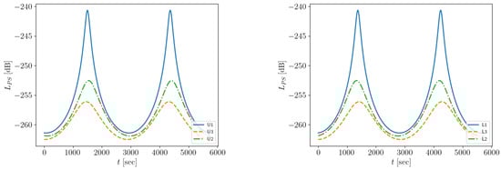
Figure 9.
Path loss variations for links established between satellite and its adjacent neighbors in the (left) upper orbit and (right) lower orbit, observed over one orbital period.
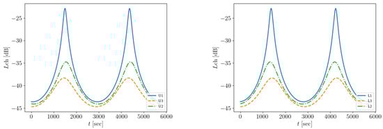
Figure 10.
Channel gain for links established between satellite and its adjacent neighbors in the (left) upper orbit and (right) lower orbit, observed over one orbital period.
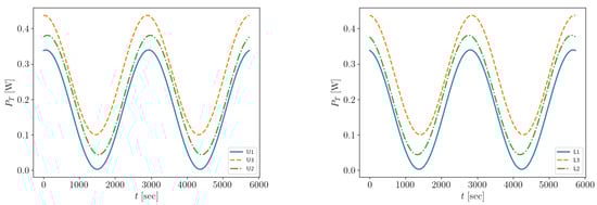
Figure 11.
Required transmission power, , for establishing links between satellite and its adjacent neighbors in the (left) upper orbit and (right) lower orbit, observed over one orbital period.
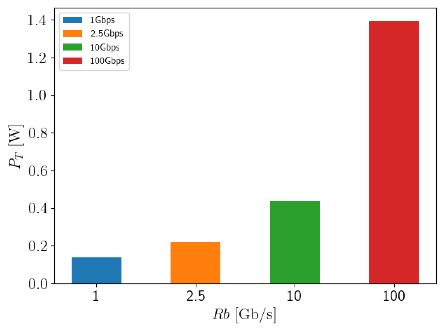
Another practical conclusion that can be drawn from these figures is the fact that, especially for neighbors in adjacent satellite orbits, the required power varies significantly over time, and hence, it may be advantageous to consider adaptive schemes to calibrate the transmission power to its required value rather than simply transmitting the maximum value obtained in the figures. Figure 12 shows how the required power scales with the specified data rate . As expected, the required optical power increases as the data rate rises. For 100 Gbps, it surpasses 1 W [41]. Note that even at such data rates, power requirements levels remain low enough to be achieved in miniaturized terminals using optically amplified transceivers [42].

Figure 12.
Maximum transmission power required to maintain connectivity between adjacent satellites as a function of the data rate, for Scenario A.
4.2. Alternative Scenarios
To further demonstrate the applicability of the Pyminisat module and assess the power requirements for minisat OILs, we explore the two alternative scenarios, B and C, outlined in Table 3. For these constellations, we first need to estimate the optimal F parameters to reduce the risk of collisions, which turns out to be for Scenario B and for Scenario C. Note that the values of the minimum distances are now 207.6 Km and 12.4 Km for Scenarios B and C, respectively. This is in accordance with the fact that constellation B is thinner than A while C is denser than A.
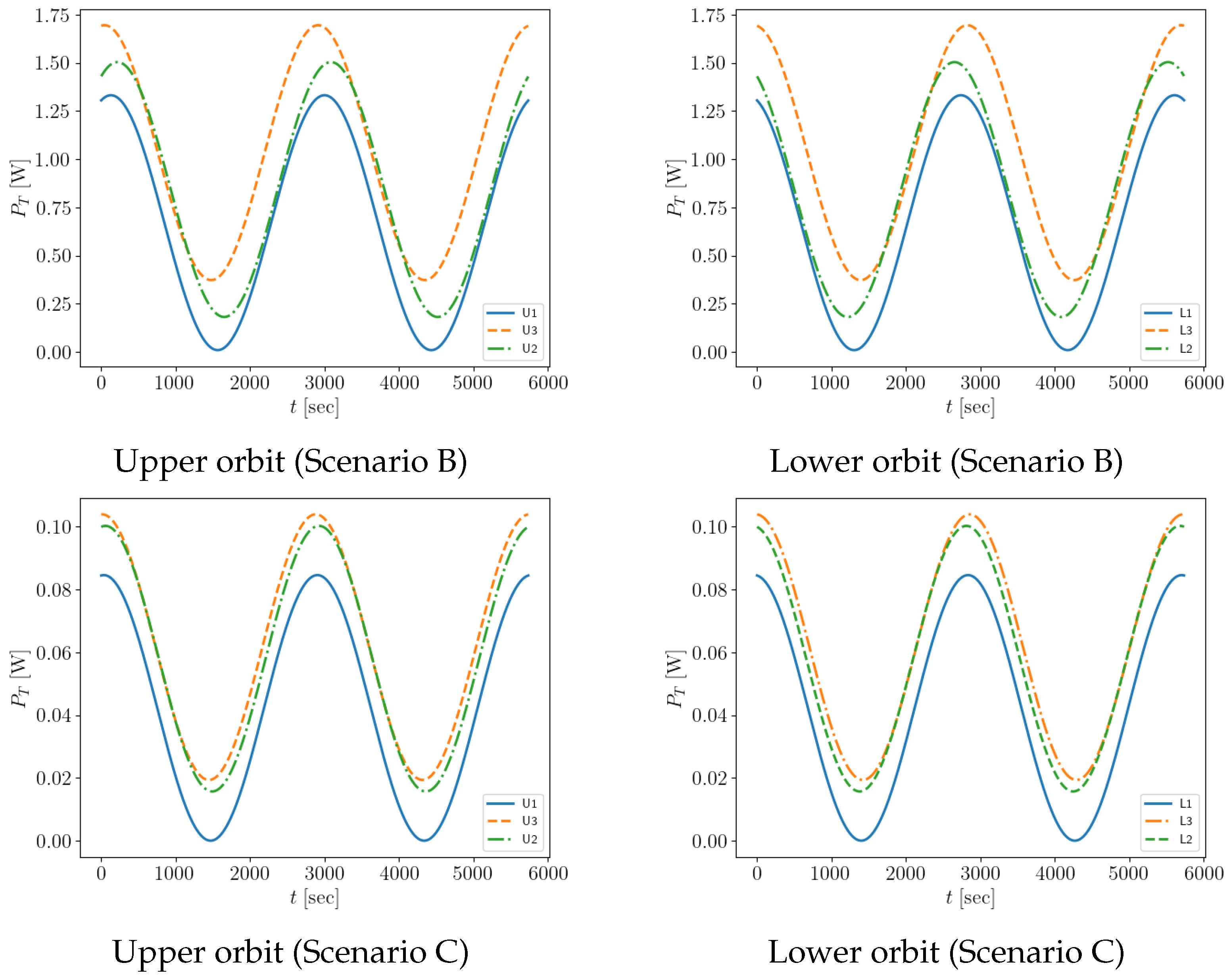
After determining the optimal F value, we applied the model to determine the link budget conditions and power requirements. Figure 13 depicts the required power to maintain the adjacent satellite links within one orbital period for both Scenarios B and C. We again assume a target data rate of 10 Gbps. In Scenario B, the optical power ranges from ≈400 mW to ≈1.7 W. For Scenario C, the range of the required power decreases significantly due to the higher constellation density, from ≈20 mW to ≈100 mW, respectively. The power levels of the latter scenario can, in principle, be supported using commercial high-power DFB lasers without optical amplification. This can simplify optical terminal implementation and improve power consumption.
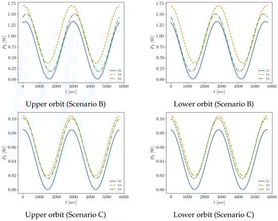
Figure 13.
Transmission power required, , for establishing links between satellite and its adjacent neighbors over one orbital period: (left) neighbors in the upper orbit and (right) neighbors in the lower orbit, for scenarios B and C.
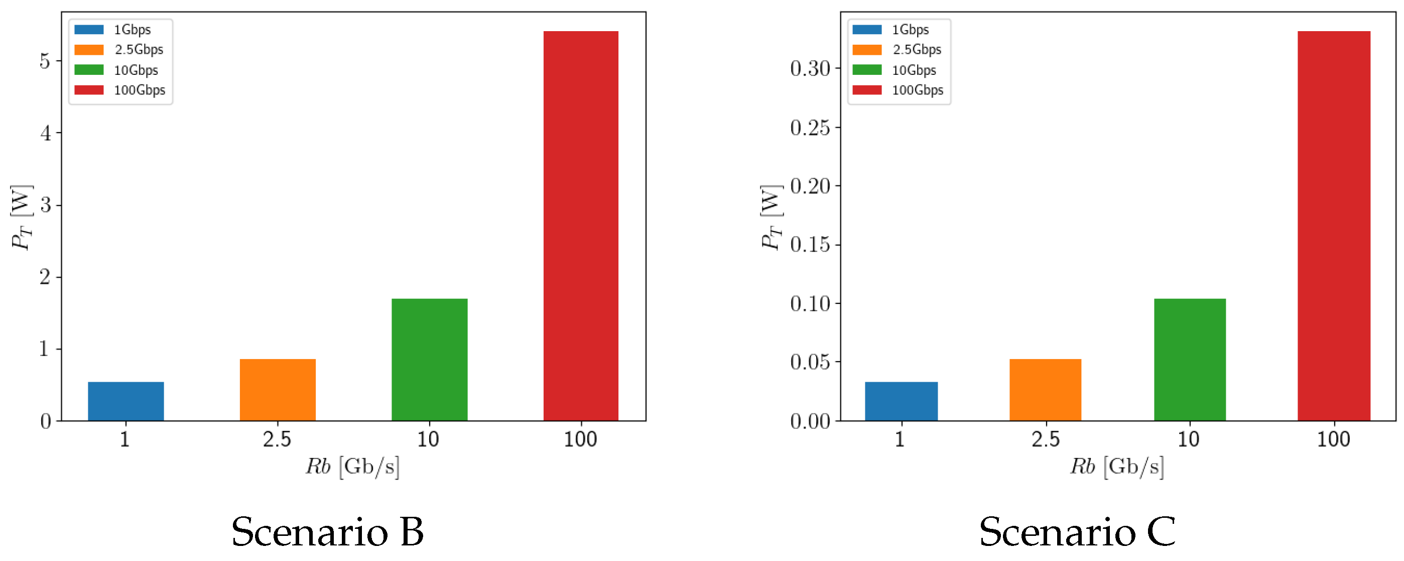
In Figure 14, we show how the maximum required power varies with the data rate for both scenarios. The figure is indicative of the bearing of constellation density in transceiver design. For Scenario B, the optical power ranges above 1 W for larger than 2.5 Gbps, reaching more than 5 W at 100 Gbps. This can pose some strict requirements at the transmitter side and especially the optical amplifier stage. Restrictions are significantly relaxed for the denser constellation of Scenario C where the transmission power reaches ≈300 mW at 100 Gbps. Such optical power levels can be supported with specially designed DFB lasers [25], thereby mitigating the need for optical amplification. The figure suggests that for this constellation, maintaining OILs at tenths of Gbps is practically feasible without excessive power requirements. One can extend the inter-satellite connection data rate using wavelength and/or polarization multiplexing to reach capacities in the Tbps realm.
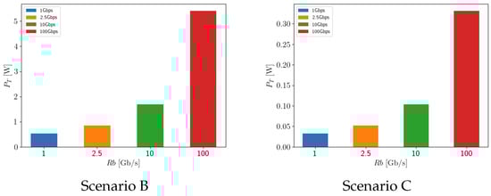
Figure 14.
Maximum transmission power required to maintain connectivity between adjacent satellites as a function of the data rate, for Scenarios B and C, as described in Table 3.
5. Conclusions and Outlook
In this work, we present a complete physical layer tool for estimating the performance of OILs in LEO satellite networks. Our tool includes various aspects, including the architecture of the constellation, link budget analysis, collision avoidance optimization, transceiver optics design, etc., and it can be used to analyze practical constellation implementations. A Python implementation of our tool is publicly available on the world-wide web under an open-source license. Using our approach, we estimated the power requirements of high-speed OIL communication assuming LEO constellation variations. We show that, especially for dense constellations, power requirements are compatible with existing state-of-the-art optical terminals even for smaller satellite sizes, pointing out the significant potential of optical satellite communications for providing high-speed network satellite internet services. Our simulation tool can be used to ascertain the feasibility of satellite network designs accurately and efficiently.
Future research could explore several promising directions, many of which we plan to address in subsequent work. While our model assumes a standard IM/DD OOK transceiver, incorporating alternative modulation formats (e.g., multi-level amplitude modulation), as well as wavelength, spatial, or polarization multiplexing, would offer valuable insights. Extending the model to coherent systems is also a promising avenue, given the power efficiency of coherent detection [43] and its support for advanced modulation formats such as PSK and QAM. Furthermore, investigating higher-network-layer design and routing algorithms could provide key insights into performance metrics such as network latency. The evaluation of optical downlink and uplink technologies under realistic conditions is also of great importance for formulating a roadmap for the advancement of these technologies. Although our study focuses on OOK, our model, which approximates an AWGN system with a time-varying path loss, can be extended to other modulation schemes, including coherent detection. Therefore, improvements in SNR and spectral efficiency observed in conventional optical systems should also be applicable in this context. Finally, future work could investigate perturbation effects (e.g., gravitational forces, drag, and station-keeping maneuvers) on acquisition, tracking, and laser alignment, as well as the impact of satellites’ structural elements such as solar panels in dense constellations, and scenarios involving uplink and downlink under turbulence effects. These studies could optimize satellite design and improve communication and tracking efficiency.
Author Contributions
M.G. was responsible for the investigation, methodology, development of models and software, original draft writing, review and editing, visualization, and data curation. T.K. contributed to the development of models and software, writing, supervision of the research activity, project administration, and participated in the review and editing process. D.A. led the conceptualization, the formulation and development of the overarching research goals and aims, and contributed to the review and editing of the manuscript. All authors have read and agreed to the published version of the manuscript.
Funding
This research received no external funding.
Institutional Review Board Statement
Not applicable.
Informed Consent Statement
Not applicable.
Data Availability Statement
The data are contained within the article.
Conflicts of Interest
The authors declare no conflicts of interest.
Appendix A. Pyminisat Module Implementation
The various model elements discussed in Section 2 and Section 3 were implemented as part of the Pyminisat Python module [28], which is publicly available under an open-source license. In its implementation, we exclusively used standard Python libraries, such as numpy, scipy for numerical manipulations, and matplotlib for result visualization. The Pyminisat module implements the satsim class, which contains all essential attributes of the satellite network pertaining to the constellation and transceiver systems. The satsim class invokes two sub-modules, namely the linkmodel class, which can be used to study an end-to-end OIL, and the constellation class, which incorporates the constellation dynamics and determines the optimal F value and the minimum distances that need to be covered in order to ensure network connectivity.
To study a given constellation, e.g., the one described in Table 1, the satsim class carries out the simulation in the following steps: first use the constellation class to estimate the best value for F and, therefore, determine the initial satellite position in the constellation. Then, initialize the constellation with the optimal value of F and calculate the minimum link distances required to provide connectivity to the nearby neighboring satellites (see Figure 4) over one orbital period. Given the parameters of the receiver and the data rate, use the linkmodel class to calculate the receiver sensitivity. Based on this value, calculate the required transmitter power for each instance of the orbital period using the link budget in (11). The Github repository of the model [28] further describes how the initialization parameters of the satsim class can be changed to fit various network scenarios.
To the extent possible, we optimized the code in order to take advantage of the large speed-ups involved when numpy vectorization is used instead of for loops. By far the most computationally challenging task is to optimize the constellation in terms of the F parameter. We can take advantage of the fact that the estimation of the distances in (9) is an embarrassingly parallel problem for the different time instances assumed. We can, therefore, use Python’s multiprocessing module to distribute the load to the available central processing unit (CPU) cores. On a standard 6-core, AMD Ryzen 5 7530U CPU (with 2 threads per core), the time required to optimize the constellation in Table 1 and estimate the power requirements is ≈ s. For completeness, we tested a scenario with a constellation even denser than Scenario C, tripling both the number of satellites per orbit and the total number of orbits compared to Scenario A, yielding a total of 14,256 satellites. The computation time required in the same platform was now 165.7 s.
References
- Carrizo, C.; Knapek, M.; Horwath, J.; Gonzalez, D.D.; Cornwell, P. Optical inter-satellite link terminals for next generation satellite constellations. In Proceedings of the Free-Space Laser Communications XXXII, San Francisco, CA, USA, 1–6 February 2020; SPIE: Bellingham, WA, USA, 2020; Volume 11272, pp. 8–18. [Google Scholar]
- Kemih, K.; Yaiche, Y.; Benslama, M. Optimization of Transmitter Aperture by Genetic Algorithm in Optical Satellite. World Acad. Sci. Eng. Technol. Int. J. Electr. Comput. Energetic Electron. Commun. Eng. 2007, 1, 1261–1267. [Google Scholar]
- Kim, G.N.; Park, S.Y.; Seong, S.; Choi, J.Y.; Han, S.K.; Kim, Y.E.; Choi, S.; Lee, J.; Lee, S.; Ryu, H.G.; et al. Design of Novel Laser Crosslink Systems Using Nanosatellites in Formation Flying: The VISION. Aerospace 2022, 9, 423. [Google Scholar] [CrossRef]
- Zhu, Q.; Tao, H.; Cao, Y.; Li, X. Laser inter-satellite link visibility and topology optimization for mega constellation. Electronics 2022, 11, 2232. [Google Scholar] [CrossRef]
- Liang, J.; Chaudhry, A.U.; Erdogan, E.; Yanikomeroglu, H. Link Budget Analysis for Free-Space Optical Satellite Networks. In Proceedings of the 2022 IEEE 23rd International Symposium on a World of Wireless, Mobile and Multimedia Networks (WoWMoM), Belfast, UK, 14–17 June 2022; pp. 471–476. [Google Scholar]
- Liang, J.; Chaudhry, A.U.; Erdogan, E.; Yanikomeroglu, H.; Kurt, G.K.; Hu, P.; Ahmed, K.; Martel, S. Free-Space Optical (FSO) Satellite Networks Performance Analysis: Transmission Power, Latency, and Outage Probability. IEEE Open J. Veh. Technol. 2024, 5, 244–261. [Google Scholar] [CrossRef]
- Space Exploration Holdings, LLC. SpaceX Non-Geostationary Satellite System, Attachment A, Technical Information to Supplement Schedule S; FCC: Washington, DC, USA, 2018; Available online: https://fcc.report/IBFS/SAT-MOD-20181108-00083/1569860.pdf (accessed on 6 December 2023).
- Carrasco-Casado, A.; Biswas, A.; Fields, R.; Grefenstette, B.; Harrison, F.; Sburlan, S.; Toyoshima, M. Optical communication on CubeSats—Enabling the next era in space science. In Proceedings of the 2017 IEEE International Conference on Space Optical Systems and Applications (ICSOS), Naha, Japan, 14–16 November 2017; pp. 46–52. [Google Scholar] [CrossRef]
- Goorjian, P.M. Free-space optical communication for spacecraft and satellites, including cubesats in low earth orbit (LEO). In Proceedings of the Photonic Networks and Devices, Burlingame, CA, USA, 29 July–1 August 2019; Optica Publishing Group: Washington, DC, USA, 2019; p. paper NeM2D.4. [Google Scholar]
- Saathof, R.; Crowcombe, W.; Kuiper, S.; van der Valk, N.; Pettazzi, F.; de Lange, D.; Kerkhof, P.; van Riel, M.; de Man, H.; Truyens, N.; et al. Optical satellite communication space terminal technology at TNO. In Proceedings of the International Conference on Space Optics—ICSO 2018, Chania, Greece, 9–12 October 2018; Sodnik, Z., Karafolas, N., Cugny, B., Eds.; International Society for Optics and Photonics, SPIE: Bellingham, WA, USA, 2019; Volume 11180, p. 111800K. [Google Scholar] [CrossRef]
- Benzi, E.; Troendle, D.C.; Shurmer, I.; James, M.; Lutzer, M.; Kuhlmann, S. Optical inter-satellite communication: The Alphasat and Sentinel-1A in-orbit experience. In Proceedings of the 14th International Conference on Space Operations, Daejeon, Republic of Korea, 16–20 May 2016; p. 2389. [Google Scholar]
- Li, L.; Zhang, X.; Zhang, J.; Xu, C.; Jin, Y. Advanced space laser communication technology on cubesats. ZTE Commun. 2021, 18, 45–54. [Google Scholar]
- Schmidt, C.; Rödiger, B.; Rosano, J.; Papadopoulos, C.; Hahn, M.T.; Moll, F.; Fuchs, C. DLR’s Optical Communication Terminals for CubeSats. In Proceedings of the 2022 IEEE International Conference on Space Optical Systems and Applications (ICSOS), Kyoto, Japan, 28–31 March 2022; pp. 175–180. [Google Scholar] [CrossRef]
- Velazco, J.; Boyraz, O. High data rate inter-satellite omnidirectional optical communicator. In Proceedings of the 32 Annual AIAA/USU Conference on Small Satellites, Logan, UT, USA, 4–9 August 2018. [Google Scholar]
- Zaman, I.U.; Velazco, J.E.; Boyraz, O. Omnidirectional optical crosslinks for CubeSats: Transmitter optimization. IEEE Trans. Aerosp. Electron. Syst. 2020, 56, 4556–4566. [Google Scholar] [CrossRef] [PubMed]
- Saeed, N.; Almorad, H.; Dahrouj, H.; Al-Naffouri, T.Y.; Shamma, J.S.; Alouini, M.S. Point-to-Point Communication in Integrated Satellite-Aerial 6G Networks: State-of-the-Art and Future Challenges. IEEE Open J. Commun. Soc. 2021, 2, 1505–1525. [Google Scholar] [CrossRef]
- Chaudhry, A.U.; Yanikomeroglu, H. Free Space Optics for Next-Generation Satellite Networks. IEEE Consum. Electron. Mag. 2021, 10, 21–31. [Google Scholar] [CrossRef]
- Liang, J.; Chaudhry, A.U.; Yanikomeroglu, H. Phasing parameter analysis for satellite collision avoidance in starlink and kuiper constellations. In Proceedings of the 2021 IEEE 4th 5G world forum (5GWF), Montreal, QC, Canada, 13–15 October 2021; IEEE: Piscataway, NJ, USA, 2021; pp. 493–498. [Google Scholar]
- Chaudhry, A.U.; Yanikomeroglu, H. Laser Intersatellite Links in a Starlink Constellation: A Classification and Analysis. IEEE Veh. Technol. Mag. 2021, 16, 48–56. [Google Scholar] [CrossRef]
- Chaudhry, A.U.; Yanikomeroglu, H. Temporary laser inter-satellite links in free-space optical satellite networks. IEEE Open J. Commun. Soc. 2022, 3, 1413–1427. [Google Scholar] [CrossRef]
- Liang, J.; Chaudhry, A.U.; Chinneck, J.W.; Yanikomeroglu, H.; Kurt, G.K.; Hu, P.; Ahmed, K.; Martel, S. Latency Versus Transmission Power Trade-Off in Free-Space Optical (FSO) Satellite Networks with Multiple Inter-Continental Connections. IEEE Open J. Commun. Soc. 2023, 4, 3014–3029. [Google Scholar] [CrossRef]
- Handley, M. Delay is Not an Option: Low Latency Routing in Space. In Proceedings of the 17th ACM Workshop on Hot Topics in Networks, Redmond, WA, USA, 15–16 November 2018; HotNets ’18. pp. 85–91. [Google Scholar] [CrossRef]
- Perlot, N.; Sofieva, V.F. Qualifying optical inter-satellite links for atmospheric occultations. In Proceedings of the International Conference on Space Optical Systems, Tokyo, Japan, 9–12 November 2009. [Google Scholar]
- Walker, J.G. Satellite constellations. J. Br. Interplanet. Soc. 1984, 37, 559. [Google Scholar]
- Wenzel, H.; Klehr, A.; Braun, M.; Bugge, F.; Erbert, G.; Fricke, J.; Knauer, A.; Ressel, P.; Sumpf, B.; Weyers, M.; et al. Design and realization of high-power DFB lasers. In Proceedings of the Physics and Applications of Optoelectronic Devices, Philadelphia, PA, USA, 25–28 October 2004; SPIE: Bellingham, WA, USA, 2004; Volume 5594, pp. 110–123. [Google Scholar]
- McDowell, J.C. The low earth orbit satellite population and impacts of the SpaceX Starlink constellation. Astrophys. J. Lett. 2020, 892, L36. [Google Scholar] [CrossRef]
- Kotake, H.; Abe, Y.; Fuse, T.; Kubooka, T.; Toyoshima, M. Adaptive optical satellite network architecture. In Proceedings of the International Conference on Space Optics—ICSO 2020, Online, 30 March–2 April 2021; SPIE: Bellingham, WA, USA, 2021; Volume 11852, pp. 685–693. [Google Scholar]
- Gioulis, M.; Kamalakis, T. Pyminisat: A Python Package for Simulating Optical Intersatellite Links in a Minisat Constellation. 2024. Available online: https://github.com/thomaskamalakis/pyminisat (accessed on 22 April 2024).
- Curtis, H.D. Orbital Mechanics for Engineering Students, 7th ed.; Elsevier Butterworth Heinemann: Oxford, UK, 2005. [Google Scholar]
- Sumathi, K.; Balasaraswathi, M.; Boopathi, C.; Singh, M.; Malhotra, J.; Dhasarathan, V. Design of 3.84 Tbps hybrid WDM–PDM based inter-satellite optical wireless communication (IsOWC) system using spectral efficient orthogonal modulation scheme. J. Ambient Intell. Humaniz. Comput. 2020, 11, 4167–4175. [Google Scholar] [CrossRef]
- Chaudhary, S.; Chaudhary, N.; Sharma, S.; Choudhary, B. High speed inter-satellite communication system by incorporating hybrid polarization-wavelength division multiplexing scheme. J. Opt. Commun. 2017, 39, 87–92. [Google Scholar] [CrossRef]
- Betti, S.; Carrozzo, V.; Parca, G. Optical Intersatellite hybrid network links based on WDM technology. In Proceedings of the 2008 10th Anniversary International Conference on Transparent Optical Networks, Athens, Greece, 22–26 June 2008; IEEE: Piscataway, NJ, USA, 2008; Volume 4, pp. 209–212. [Google Scholar]
- Horst, Y.; Bitachon, B.I.; Kulmer, L.; Brun, J.; Blatter, T.; Conan, J.M.; Montmerle-Bonnefois, A.; Montri, J.; Sorrente, B.; Lim, C.B.; et al. Tbit/s line-rate satellite feeder links enabled by coherent modulation and full-adaptive optics. Light. Sci. Appl. 2023, 12, 153. [Google Scholar] [CrossRef]
- Ramaswami, R.; Sivarajan, K.N.; Sasaki, G.H. Optical Networks, A Practical Perspective, 3rd ed.; Elsevier: Amsterdam, The Netherlands, 2010. [Google Scholar]
- Vieira, I.P.; Pita, T.C.; Mello, D.A.A. Modulation and Signal Processing for LEO-LEO Optical Inter-Satellite Links. IEEE Access 2023, 11, 63598–63611. [Google Scholar] [CrossRef]
- Brashears, T.R. Achieving 99% link uptime on a fleet of 100G space laser inter-satellite links in LEO. In Proceedings of the Free-Space Laser Communications XXXVI, San Francisco, CA, USA, 27 January–1 February 2024; SPIE: Bellingham, WA, USA, 2024; Volume 12877, p. 1287702. [Google Scholar]
- Kato, W.; Kawamoto, Y.; Kato, N.; Ariyoshi, M.; Sugyo, K.; Funada, J. Stable and Efficient Inter-Satellite Optical Wireless Communications Through Connection of Intersecting Orbits. In Proceedings of the 2024 IEEE 99th Vehicular Technology Conference (VTC2024-Spring), Singapore, 24–27 June 2024; IEEE: Piscataway, NJ, USA, 2024; pp. 1–5. [Google Scholar]
- Zhu, Y.; Xu, G.; Gao, M.; Chu, H.; Song, Z. Average bit-error rate analysis of an inter-satellite optical communication system under the effect of perturbations. Opt. Express 2024, 32, 36796–36810. [Google Scholar] [CrossRef]
- Stampoulidis, L.; Osman, A.; Sourikopoulos, I.; Winzer, G.; Zimmermann, L.; Dorward, W.; Rodrigo, A.S.; Chiesa, M.; Rotta, D.; Maho, A.; et al. H2020-SPACE-ORIONAS Miniaturized optical transceivers for high-speed optical inter-satellite links. arXiv 2022, arXiv:2210.17304. [Google Scholar]
- Rödiger, B.; Fuchs, C.; Nonay, J.R.; Jung, W.; Schmidt, C. Miniaturized optical Intersatellite communication terminal–CubeISL. In Proceedings of the 2021 IEEE International Conference on Communications Workshops (ICC Workshops), Montreal, QC, Canada, 14–23 June 2021; IEEE: Piscataway, NJ, USA, 2021; pp. 1–5. [Google Scholar]
- Edmunds, J.; Thipparapu, N.; Kechagias, M.; Hall, K.; Donnot, A.; Kean, P.; Kehayas, E.; Welch, M. Designing transmit optical amplifiers for the current roll out of optical communication constellations. In Proceedings of the International Conference on Space Optics—ICSO 2022, Dubrovnik, Croatia, 3–7 October 2022; SPIE: Bellingham, WA, USA, 2023; Volume 12777, pp. 1497–1504. [Google Scholar]
- Carrasco-Casado, A.; Shiratama, K.; Kolev, D.; Trinh, P.V.; Ishola, F.; Fuse, T.; Toyoshima, M. Development and space-qualification of a miniaturized CubeSat’s 2-W EDFA for space laser communications. Electronics 2022, 11, 2468. [Google Scholar] [CrossRef]
- Morthier, G.; Roelkens, G.; Baets, R. Optical versus RF free-space signal transmission: A comparison of optical and RF receivers based on noise equivalent power and signal-to-noise ratio. IEEE J. Sel. Top. Quantum Electron. 2021, 28, 1–8. [Google Scholar] [CrossRef]


Disclaimer/Publisher’s Note: The statements, opinions and data contained in all publications are solely those of the individual author(s) and contributor(s) and not of MDPI and/or the editor(s). MDPI and/or the editor(s) disclaim responsibility for any injury to people or property resulting from any ideas, methods, instructions or products referred to in the content. |
© 2025 by the authors. Licensee MDPI, Basel, Switzerland. This article is an open access article distributed under the terms and conditions of the Creative Commons Attribution (CC BY) license (https://creativecommons.org/licenses/by/4.0/).