Exact Solutions to Cancer Laser Ablation Modeling

Abstract

The present paper deals with the study of the fluence rate over both healthy and tumor tissues in the presence of focal laser ablation (FLA). We propose new analytical solutions for a coupled partial differential equation (PDE) system, which includes the transport equation modeling of light penetration into biological tissue, the bioheat equation modeling the heat transfer, and its respective damage. The present work could be the first step toward knowledge of the mathematical framework for biothermophysical problems, as well as the main key to simplify the numerical calculations due to its zero cost. We derive exact solutions and simulate results from them. We discuss the potential physical contributions and present respective conclusions about the following: (1) the validity of the diffusion approximation of the radiative transfer equation; (2) the local behavior of the source of scattered photons; (3) the unsteady state of the fluence rate; and (4) the boundedness of the critical time of the thermal damage to the cancerous tissue. We also discuss some controversial and diverging hypotheses.

1. Introduction

Thermal ablation is a widely accepted therapy for denaturing proteins and then the destruction of tissue cells. It has been used for the treatment of both atrial fibrillation [1] and cancer [2,3]. In recent decades, several energy sources have been applied (see [4,5] and references therein), including radiofrequency [6,7,8,9], microwave [10,11], cryoablation [12,13,14], ultrasound [15], and laser [16,17]. Focal laser ablation (FLA) is a minimally invasive procedure used to treat tumors using laser energy to heat and destroy cancerous cells. Indeed, FLA is gaining acceptance as a safe option and effective alternative to surgical resection; see [18,19,20] and the references therein.

An ideal hyperthermia treatment is one that selectively destroys the diseased cells without damaging the surrounding healthy tissue. For this reason, it is still essential to build analytical solutions to hold up such selective targeting. The FLA model results from three distinct phenomena: the conversion of laser light into heat, the transfer of heat, and coagulation necrosis. It consists of a coupled partial differential equation (PDE) system that includes a diffusion approximation of the radiative transfer equation modeling the light penetration into biological tissue, the Pennes bioheat transfer equation modeling the heat transfer, and the Arrhenius burn integration modeling the dimensionless indicator of the damage. The worldwide literature on the heat transfer in ablation modeling commonly considers the heat source as constant or of a particular profile. In FLA, the heat source, the so-called absorbed optical power density, is induced through the conversion of laser light into heat and has a well-known linear relationship with the fluence rate. In the presence of this relationship, accurate knowledge of the fluence rate is the key feature for the mathematical framework.

For a light source acting as a cylindrical diffuser, the fluence rate is obtained in terms of zero-order modified Bessel functions ([21], pp. 172–174). Also, other expressions exist (see, for instance, ref. [22] and the references therein). For a single spherically symmetric point source, we mention [21,23,24] and the references therein. The laser beam has a crater-like shape, since the intensity is not constant across the beam width but decreases from the center towards the edge [25].

Some analytical solutions to the bioheat transfer problem have been studied for RF ablation in multiregion domains [26,27,28]. We refer to [23] in which finite element model simulations of laser therapy were computed. For the skin surface in [29], the authors provided a theoretical study of the thermal wave effects in the bioheat transfer problem involving a high-heat-flux incident with a short duration. For breast tumor thermal therapy, in [15], the authors proposed cylindrical ultrasound phased array with a multifocus pattern scanning strategy. For a spherical tumor, in [8], the authors simulated the current density distribution when a 3D current density was generated with different multiple-straight-needle electrode configurations. Using finite element modeling, in [30], the authors analyzed photo-thermal heating with near-infrared radiation in the presence of intravenous blood injection or intratumorally injected gold nanorods. We refer to [31] for a study on endovenous laser ablation (EVLA), which is a similar technique used to treat varicose veins using laser energy to close off affected veins.

One-dimensional, time-dependent models for the removal of material using a laser beam were published in [25] and the references therein. The thermal penetration differs with the laser system (Argon, Nd:YAG, and CO₂ [16]). Failure rates may depend on the design of the optical fibers. In [32], the authors show that the heat-affected zone is significantly reduced using a short-pulsed laser of the same average power (150 $\mathrm{m}$$\mathrm{W}$ for 25 s) compared to a CW laser source. Short-pulsed lasers are being used in a variety of applications such as remote sensing, optical tomography, laser surgery, and ablation processes.

In the present work, we derive exact solutions and apply the resulting solutions under Nd:YAG and diode lasers for their wide application. We analyze the light source over different tissues and its tissue absorption under the Beer–Lambert (BL) law. We focus our attention on breast and prostate tumors, which are cancers commonly diagnosed in women and men worldwide [33,34].

The outline of the present work is as follows. We first describe the mathematical model in Section 2. In Section 3, we propose new exact solutions for the unknown functions under study. In Section 4, we apply the previous results to the fluence rate and temperature in Section 4.1 and Section 4.3, respectively, and present some simulation results in Section 4.2. Section 5 indicates the main interpretations of this study, and Section 6 presents the corresponding conclusions. Finally, two Appendices are included, containing mathematical proofs relative to Section 4.

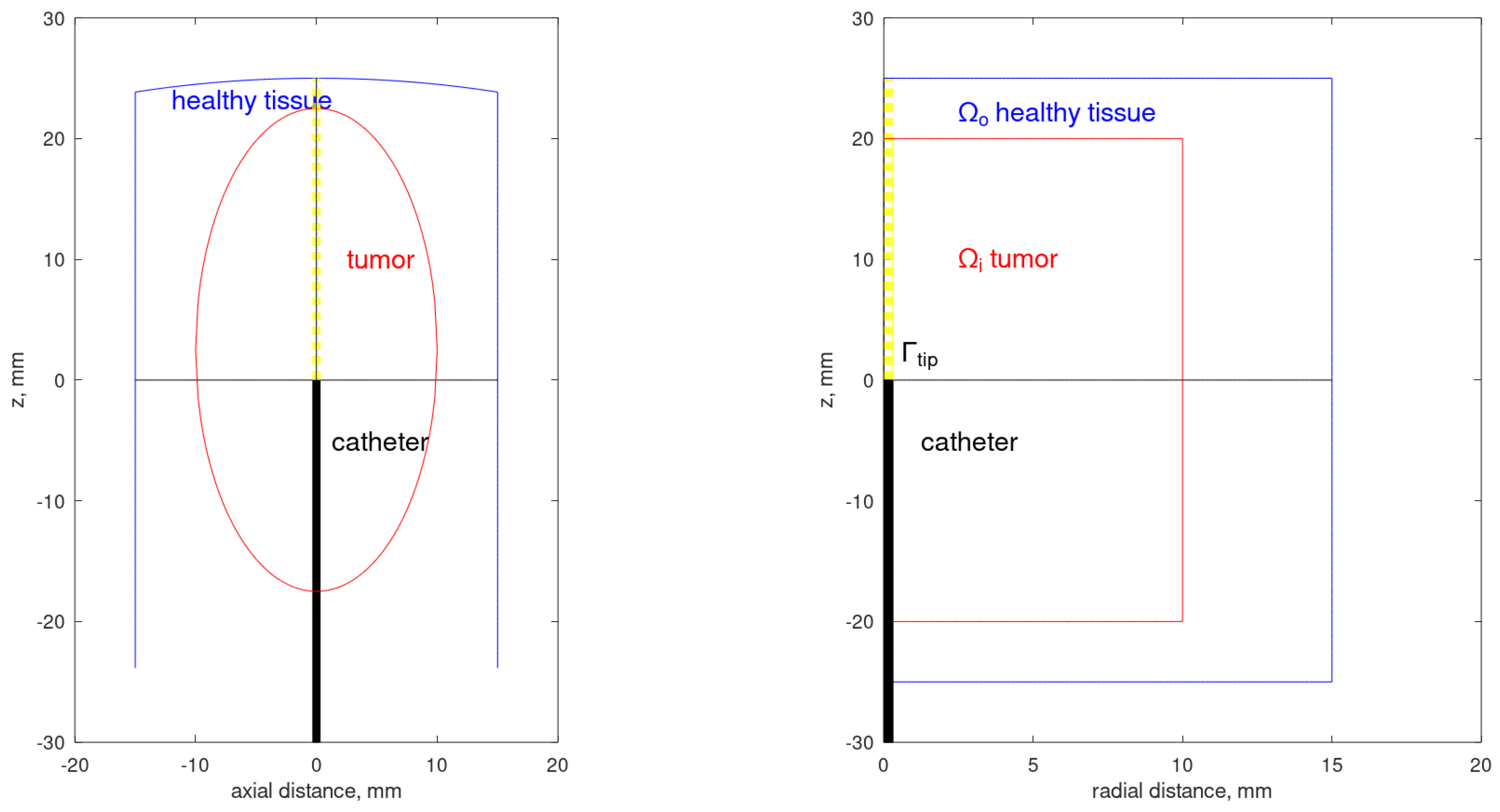
2. Mathematical Formulation

The laser applicator usually consists of an optical fiber (with radius $r_{\mathrm{f}}$) incorporated within a catheter. The diameter of the optical fiber for medical applications varies between 200 $\mathrm{\mu }$$\mathrm{m}$ and 600 $\mathrm{\mu }$$\mathrm{m}$ [35], while the laser beam diameter is 2 $\mathrm{m}$$\mathrm{m}$ [32]. Thus, we may assume $r_{\mathrm{f}}=0.25 \mathrm{m}\mathrm{m}$ [36]. The fiber–catheter system is represented along the longitudinal axis z, as shown in black in Figure 1, and is simply identified by the name catheter.

Both breast and prostate tumors can be modeled as ellipsoids (see [33,36] and references therein), as shown in Figure 1 (Left). For defining the domain of laser fluence or thermal effect, we deal with the ellipsoid shape of the tumors as usual as a cylindrical shape. We assume the geometry of the laser–tissue system to be as illustrated in Figure 1 (Right). The tumor ${\mathrm{\Omega }}_{\mathrm{i}}$ and surrounding healthy tissue ${\mathrm{\Omega }}_{\mathrm{o}}$ are represented by cylinders, with $r_{\mathrm{i}}$ and $r_{\mathrm{o}}$ as the inner and outer radius, respectively. Let us define the bidomain

$$\mathrm{\Omega }=\mathrm{int}({\overline{\mathrm{\Omega }}}_{\mathrm{i}}\cup {\mathrm{\Omega }}_{\mathrm{o}}).$$

Mean breast and prostatic carcinoma sizes may vary in different ranges. We assume the inner radius $r_{\mathrm{i}}=1 \mathrm{c}\mathrm{m}$. Although the primary goal is to destroy all malignant tissue, the surrounding nonmalignant tissue should be preserved. To evaluate this rim of surrounding tissue, the outer radius $r_{\mathrm{o}}$ will be determined such that the fluence rate vanishes. Indeed, the respective photons just “vanish” from the system due to the absorption of light reaching the system border.

The laser light is emitted from the distal end of the fiber on an active length that is approximately half the tumor size ([35], p. 82). By this reason, the distal end is assumed to be centered in the middle of the tumor; that is, the longitudinal coordinate is $-\ell <z<\ell$.

Three different instants of time are of reference: the temporal pulse width $t_p$ (also known as the pulse duration or pulse width, for short), the critical time $t_{\mathrm{crit}}$, and the exposure duration $t_{\mathrm{end}}$. The pulse width $t_p$ is the time measured across a pulse, at its full width at half maximum (FWHM). The critical time $t_{\mathrm{crit}}$ is introduced in Section 2.3. The exposure duration $t_{\mathrm{end}}$ consists of N pulse widths and $N-1$ pulse-to-pulse intervals $\Delta t$ (the so-called periods), which are ten times the pulse width [16].

2.1. Photon Transport

Photon transport is governed by the diffusion approximation of the radiative transfer equation (see, for instance, [21,35,37]):

$${\displaystyle \frac{1}{\nu }}{\partial }_t\varphi -D\Delta \varphi +{\mu }_{\mathrm{a}}\varphi =S\mathrm{in}\mathrm{\Omega }\times ]0;t_{\mathrm{end}}[,$$

(1)

where the light velocity in the tissue $\nu =c/n$. The Laplace operator $\Delta =\nabla ·\nabla$, with ∇ standing for the spatial gradient, and the time partial derivative ${\partial }_t=\partial /\partial t$.

The diffusion coefficient is

$$D={\displaystyle \frac{1}{3({\mu }_{\mathrm{a}}+{\mu }_{\mathrm{s}}^{\prime })}}.$$

Here, the reduced scattering coefficient ${\mu }_{\mathrm{s}}^{\prime }$ is a function of the wavelength $\lambda$, which is normalized by the reference wavelength 500 $\mathrm{n}$$\mathrm{m}$:

$${\mu }_{\mathrm{s}}^{\prime }=a{\left({\displaystyle \frac{\lambda }{500}}\right)}^{-b}$$

where a and b are known constants [38]. The reduced scattering coefficient ${\mu }_{\mathrm{s}}^{\prime }$ obeys ${\mu }_{\mathrm{s}}^{\prime }=(1-g){\mu }_{\mathrm{s}}$. The biological tissue is a strongly scattering medium, and then the scattering anisotropy coefficient g ranges from $0.7$ to $0.99$ for most biological tissues [35]. The optical parameters of the tissue are known (cf.

Table 1. Average optical parameters for breast and prostate (tumor and healthy) tissues [24,35,38].

		${\mathit{\mu }}_{\mathbf{a}}$	[cm−1]	a [mm−1]	b	n
$\mathbf{\lambda }$  [nm]	810	980	1064
Breast tumor	0.08	0.07	0.06	2.07	1.487	1.4
Prostate tumor	0.12	0.11	0.1	3.36	1.712	1.4
Breast tissue	0.17	0.2	0.3	1.68	1.055	1.35
Prostate tissue	0.6	0.5	0.4	3.01	1.549	1.37

), which are assumed to be temperature-independent [25]. The average of the absorption coefficient ${\mu }_{\mathrm{a}}$ and the reduced scattering coefficient ${\mu }_{\mathrm{s}}^{\prime }$ belong to the ranges of 0–0.6 and 0–20 cm⁻¹, respectively.

We consider the beam divergence to be negligible around the focus, and then the effects of the laser radiation in terms of the local absorption of light are in accordance with the Beer–Lambert law [37]. The source of the scattered photons S represents the power injected into the unit volume, and it is given by

$$S(r,z,t)={\displaystyle \frac{{\mu }_{\mathrm{s}}({\mu }_{\mathrm{t}}+g{\mu }_{\mathrm{a}})}{{\mu }_{\mathrm{a}}+{\mu }_{\mathrm{s}}^{\prime }}}E(r,t)exp[-{\mu }_{\mathrm{t}}z],$$

(2)

for $(r,z,t)\in ]0;r_{\mathrm{o}}[\times ]0;L[\times ]0;t_{\mathrm{end}}[$. Here, the total attenuation coefficient is

$${\mu }_{\mathrm{t}}={\mu }_{\mathrm{a}}+{\mu }_{\mathrm{s}}={\mu }_{\mathrm{a}}+{(1-g)}^{-1}a{(500/\lambda )}^b,$$

(3)

and the planar irradiance, over the exposure duration $t_{\mathrm{end}}$, is

$$E(r,t)={\displaystyle \frac{P_{\mathrm{peak}}}{\pi r_{\mathrm{f}}^2}}{\chi }_{[0;r_{\mathrm{f}}]}\left(r\right)\sum _{j=0}^{N-1}{\chi }_{[t_j;t_j+t_p]}\left(t\right),$$

(4)

with each pulse time $t_j=j(t_p+\Delta t)$ and ${\chi }_I$ standing for the characteristic function over the interval I. The number of pulses is $N=(t_{\mathrm{end}}+\Delta t)/(t_p+\Delta t)$.

The difference in relative refractive indices between tumor media and healthy tissue is positive, that is, the tumor refractive index $n_0=1.4>n_1$ (the refractive index of the medium of the transmitted ray). At the interfaces, where mismatched refractive indices occur, we may consider the Robin boundary conditions [37,39]:

$$\begin{array}{cc}\hfill -D{\displaystyle \frac{\partial \varphi }{\partial z}}+{\gamma }_r\varphi =-S_1& atz=\ell ;\hfill \end{array}$$

(5)

$$\begin{array}{cc}\hfill -2D{\displaystyle \frac{\partial \varphi }{\partial r}}+{\gamma }_r\varphi =0& atr=r_{\mathrm{i}}.\hfill \end{array}$$

(6)

Here, the coefficient ${\gamma }_r$ denotes a reflectance-dependent function [21,37], and

$$S_1(r,z)=g{\displaystyle \frac{{\mu }_{\mathrm{s}}}{{\mu }_{\mathrm{tr}}}}E(r,t_p)exp[-{\mu }_{\mathrm{t}}z],$$

with the transport attenuation coefficient ${\mu }_{\mathrm{tr}}={\mu }_{\mathrm{a}}+{\mu }_{\mathrm{s}}^{\prime }$. Note that the source of scattered photons $S=-\partial S_1/\partial z+S_2$ ([21], Equation (6.4)), where $S_2(r,z)={\mu }_{\mathrm{s}}\ast E(r,t_p)exp[-{\mu }_{\mathrm{t}}z]$ and

$$S_1(r,z)={\displaystyle \frac{g}{{\mu }_{\mathrm{t}}+g{\mu }_{\mathrm{a}}}}S(r,z,t_p).$$

(7)

Robin boundary conditions (5) and (6) mean that whenever light reaches the system borders, some photons are reflected back into the system.

The remaining interfaces, $z=0$ and $r=r_{\mathrm{f}}$, are indeed mathematical boundaries and not tissue borders. Thus, we assume the continuity of the fluence rate $\varphi$ and its flux.

2.2. Heat Transfer

The heat transfer due to the energy of light deposited is governed by the Pennes bioheat transfer equation that distinguishes nonliving medium:

$$\rho c_{\mathrm{p}}{\partial }_{t}T-\nabla ·(k\nabla T)+c_{\mathrm{b}}{\omega }_{\mathrm{b}}(T-T_{\mathrm{b}})=q\mathrm{in}\mathrm{\Omega }\times ]0;t_{\mathrm{end}}[,$$

(8)

where the blood perfusion rate ${\omega }_{\mathrm{b}}$ is obtained from the capillary bed. The temperature of the blood $T_{\mathrm{b}}$ is constant and assumed to be 38 °C. The blood perfusion rate ${\omega }_{\mathrm{b}}$ may have a nonlinear temperature dependence [40]. Here, we assume that ${\omega }_{\mathrm{b}}$ obeys linear time dependence (11).

The specific heat capacity per unit mass $c_{\mathrm{p}}$ and thermal conductivity k may be based on the following relationships ([35], pp. 68–69):

$$\begin{array}{cc}\hfill c_{\mathrm{p}}& =\left(1550+2800{\displaystyle \frac{{\rho }_{\mathrm{w}}}{\rho }}\right) \mathrm{J} {\mathrm{kg}}^{-1} {\mathrm{K}}^{-1};\hfill \\ \hfill k& =\left(0.06+0.57{\displaystyle \frac{{\rho }_{\mathrm{w}}}{\rho }}\right) \mathrm{W} {\mathrm{m}}^{-1} {\mathrm{K}}^{-1},\hfill \end{array}$$

where ${\rho }_{\mathrm{w}}$ denotes the density of the water. In particular, we denote the density and the specific heat capacity of the blood by ${\rho }_{\mathrm{b}}$ and $c_{\mathrm{b}}$, respectively. Furthermore, $c_{\mathrm{b}}{\omega }_{\mathrm{b}}$ accounts for the heat conducted in the direction of the contribution of flowing blood to the overall energy balance, before the critical coagulation temperature.

Metabolism behavior is neglected due to its small contribution to the temperature response. Then, the absorbed optical power density q, which stands for the laser-light-induced heat source, is governed by

$$q={\mu }_{\mathrm{a}}\varphi .$$

(9)

We refer to [41,42,43] for the thermal relaxation time in the conduction equation with both Fourier and non-Fourier effects instead of considering systems (8) and (9). In recent years, researchers have continued to propose various alternatives to the benchmark work developed by Pennes. We mention [44] and the references therein in which a local thermal non-equilibrium bioheat model was studied.

2.3. Thermal Damage to the Tissue

Thermal laser–tissue interaction exhibits four phases: coagulation, vaporization, carbonization, and melting (vacuolation) ([35], pp. 58–63).

A critical time $t_{\mathrm{crit}}$, which corresponds to the dimensionless indicator of damage when it is equal to one, $\mathrm{\Omega }\left(t_{\mathrm{crit}}\right)=1$, obeys the Arrhenius burn integration [40]

$${\displaystyle \frac{1}{A}}={\int }_0^{t_{\mathrm{crit}}}exp\left[-{\displaystyle \frac{E_{\mathrm{a}}}{RT(·,\tau )}}\right]\tau ,$$

(10)

in the domain $\mathrm{\Omega }$, where the Arrhenius factor A is also called by frequency factor.

The linear behavior of the blood perfusion rate ${\omega }_{\mathrm{b}}$ is defined by

$${\omega }_{\mathrm{b}}\left(t\right)={\omega }_0(1-t/t_{\mathrm{crit}}),\mathrm{for}0\le t\le t_{\mathrm{crit}},$$

(11)

with ${\omega }_0={\rho }_{\mathrm{b}}w$ denoting the initial value of the blood perfusion. We recall that the volumetric flow w stands for the volume of blood per second that flows through a unit volume of tissue, with an SI unit of 1/s, which means (m³/s)/m³. The blood perfusion rate ${\omega }_{\mathrm{b}}$ is set to zero if there is no blood perfusion, which is the case for $t>t_{\mathrm{crit}}$.

3. Analytical Solutions

Our objective is to build exact solutions that fit, specifically, the physiological problem under study,

$$\tau {\partial }_{t}u-\alpha \Delta u+Bu=f,$$

(12)

using the separable variable method in cylindrical coordinates, i.e., at position $(r,z)$ and time t. Using the Bernoulli–Fourier technique, we have

$$\left(\tau X^{\prime }\left(t\right)+[-\alpha (\beta +{\eta }^2)+B]X\left(t\right)\right)R\left(r\right)Z\left(z\right)=f(r,z,t),$$

(13)

where constants $\beta ,\eta \in \mathbb{R}$ are arbitrary,

• Radiative transfer: $\tau =1/\nu$, $\alpha =D$, $B={\mu }_{\mathrm{a}}$, and $f=S$ in Section 2.1;
• Heat transfer: $\tau =\rho c_{\mathrm{p}}$, $\alpha =k$, $B=c_{\mathrm{b}}{\omega }_{\mathrm{b}}\left(t\right)$, and $f=q$ in Section 2.2.

Functions X, Z, and R are elementary solutions to the system of ordinary differential equations (ODEs):

$$\left\{\begin{array}{c}{X}^{\prime }\left(t\right)=\zeta X\left(t\right)\hfill \\ Z^{″}\left(z\right)={\eta }^{2}Z\left(z\right)\hfill \\ {\left(r{R}^{\prime }\left(r\right)\right)}^{\prime }=\beta rR\left(r\right)\hfill \end{array}\right.$$

(14)

for some time parameter $\zeta \in \mathbb{R}$. The nonconstant behavior of ${\omega }_{\mathrm{b}}$ (cf. (11)) does not invalidate the application of this technique in determining an analytical solution for the heat transfer.

Firstly, a particular solution is available due to the Duhamel principle (for details, see [31] and the references therein). Secondly, let us search for elementary solutions for the ODE system (14).

The first-order ODE in (14) admits the elementary solution

$$X\left(t\right)=exp\left[{\int }_0^t\zeta \left(s\right)s\right],t>0.$$

(15)

The second-order ODE in (14), with constant coefficients, admits the elementary solutions

$$Z\left(z\right)=exp\left[\pm \eta z\right],z\in \mathbb{R}.$$

(16)

The second-order ODE in (14), with nonconstant coefficients, admits the Bessel functions of the first and second kind and of order 0, respectively, $J_0\left(\sqrt{\left|\beta \right|}r\right)$ and $Y_0\left(\sqrt{\left|\beta \right|}r\right)$, if $\beta <0$; or the modified Bessel functions of the first and second kind and of order 0, respectively, $I_0\left(\sqrt{\beta }r\right)$ and $K_0\left(\sqrt{\beta }r\right)$, if $\beta >0$ [45]. If $\beta =0$, the elementary solutions reduce to $R\left(r\right)=log\left[r\right]$ and the unity function.

Then, a general solution solving homogeneous Equation (13) ($f=0$) is available through the above elementary solutions if

$$\tau \zeta +B=\alpha (\beta +{\eta }^2).$$

(17)

Finally, we analyze PDE (12) at the period of time $0<t_j+t_p<t<t_{j+1}$, for any $j=0,\cdots ,N-1$. This case will describe the homogeneous problem, which is governed without a source ($f=0$) at one pulse-to-pulse interval $\Delta t$. For the sake of simplicity, we denote the initial instant of time $t_j+t_p$ by $t_0$ throughout this section.

For the initial condition $u(r,z,t_0)=u_{0}Z(\eta ;z)$, where $Z(\eta ;z)$ denotes a linear combination of the elementary solutions Z given as in (16), we apply the principle of superposition ([45], Chapter 3–4) to obtain the solution in the form of the Fourier–Bessel series:

$$u(r,z,t)=\sum _{m=1}^{\infty }{c}_m{J}_0\left(b_{m}r\right)Z(\eta ;z)exp\left[{\zeta }_m(t-t_0)\right]$$

(18)

which satisfies homogeneous PDE (12) ($f=0$) in a solid cylinder ($0<r<a$) with finite length L. The zero-order Bessel function of the second kind, $Y_0$, is excluded from the solution because the region includes the origin $r=0$, where $Y_0$ becomes infinite.

We adapt the homogeneous problems for heat equation ($B=0$) in $(r,z,t)$ variables ([45], pp. 127–131), namely Example 3–9 for a hollow cylinder of finite length and Example 3–10 for a solid cylinder of semi-infinite length.

To determine the coefficients $c_m$, we multiply both sides of (18) by $r{J}_0\left(b_{n}r\right)$ and integrate over the section of the cylinder, obtaining

$$u_0{\int }_0^{a}r{J}_0\left(b_{n}r\right)r=c_n{\int }_0^{a}r{J}_0^2\left(b_{n}r\right)r.$$

On the left-hand side, we used the initial condition, and on the right-hand side, we applied the orthogonality relationship of the eigenfunctions:

$${\int }_0^{a}r{J}_0\left(b_{m}r\right)J_0\left(b_{n}r\right)r={\delta }_{m,n}{\int }_0^{a}r{J}_0\left(b_{m}r\right)J_0\left(b_{n}r\right)r$$

(19)

where ${\delta }_{m,n}$ is the Kronecker delta and the eigenvalues $b_m$ are determined by the boundary condition.

For any $a,b>0$, by integration, we have the following ([45], Appendix IV):

$$\begin{array}{cc}\hfill {\int }_0^{a}r{J}_0\left(br\right)r=& {\displaystyle \frac{a}{b}}{J}_1\left(ba\right);\hfill \\ \hfill {\int }_0^{a}r{J}_0^2\left(br\right)r=& {\displaystyle \frac{a^2}{2}}\left(J_0^2\left(ba\right)-J_{-1}\left(ba\right)J_1\left(ba\right)\right).\hfill \end{array}$$

Recall that $W_{-1}\left(a\right)=-W_1\left(a\right)$ for any Bessel function of zero order, $W=J_0,Y_0,K_0,I_0$.

Then, the complete solution is

$$u(r,z,t)=\sum _{n=1}^{\infty }{u}_0{\displaystyle \frac{2}{b_{n}a}}{\displaystyle \frac{J_1\left(b_{n}a\right)}{J_0^2\left(b_{n}a\right)+J_1^2\left(b_{n}a\right)}}{J}_0\left(b_{n}r\right)Z(\eta ;z)exp\left[{\zeta }_n(t-t_0)\right].$$

(20)

4. Results

We focus on the study of the analytical solution for the fluence rate $\varphi$ in this section. We derive an exact solution in Section 4.1 and its applicability in Section 4.2. This section ends with some considerations for the temperature and respective tissue damage in Section 4.3.

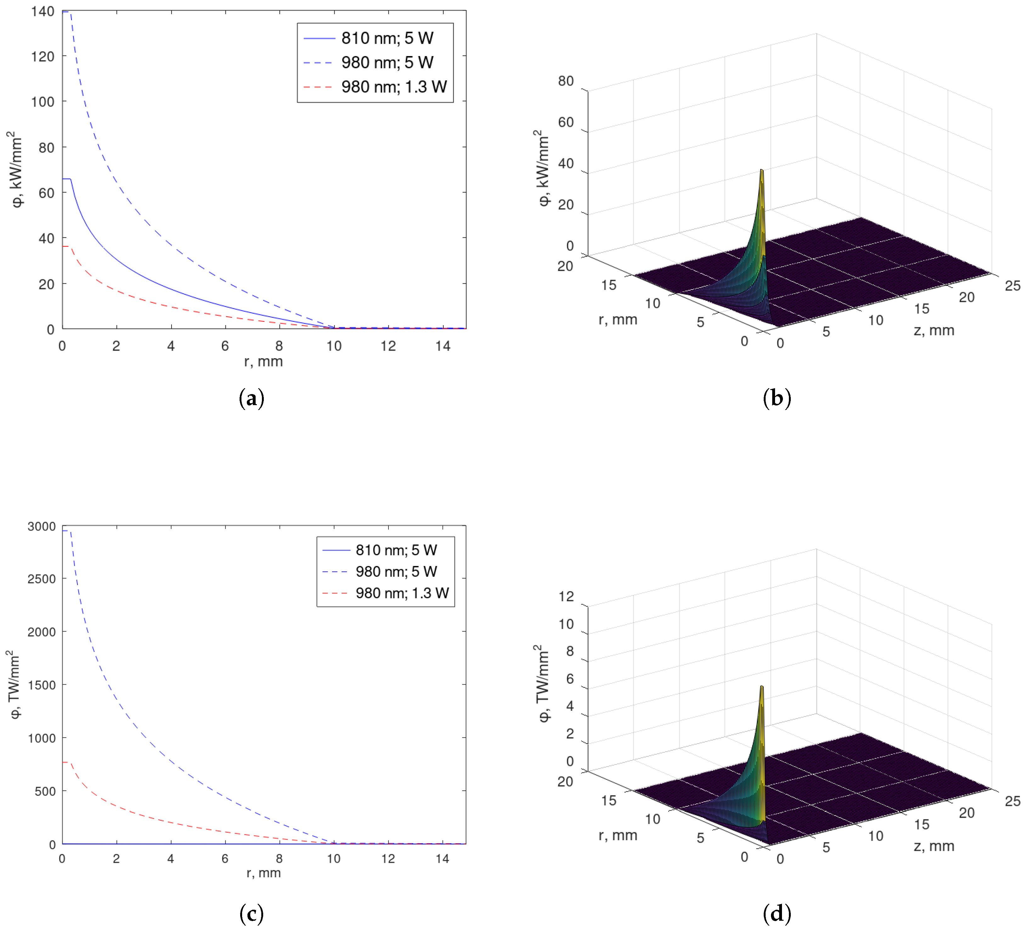
4.1. Exact Solution for the Fluence Rate $\varphi$

The time parameter in (17) is

$$\zeta =\nu (D{\mu }_{\mathrm{t}}^2-{\mu }_{\mathrm{a}})={\displaystyle \frac{c}{n}}\left({\displaystyle \frac{{({\mu }_{\mathrm{a}}+{(1-g)}^{-1}a{(500/\lambda )}^b)}^2}{3({\mu }_{\mathrm{a}}+a{(500/\lambda )}^b)}}-{\mu }_{\mathrm{a}}\right).$$

(21)

We denote $\zeta$ by ${\zeta }_{\mathrm{in}}$ in the tumor and ${\zeta }_{\mathrm{out}}$ in the healthy tissue. According to Table 1, ${\zeta }_{\mathrm{in}}>0$.

For $0\le r\le r_{\mathrm{f}}$, $0\le z\le \ell$, and $0\le t<t_p$, the transient solution of (1)–(2) is

$${\varphi }_f(z,t)\equiv {\displaystyle \frac{S(r_{\mathrm{f}},z,0)}{D{\mu }_{\mathrm{t}}^2-{\mu }_{\mathrm{a}}}}\left(exp\left[{\zeta }_{\mathrm{in}}t\right]-1\right).$$

(22)

Hereafter, let us set

$$S_{\mathrm{in}}={\displaystyle \frac{S(r_{\mathrm{f}},0,0)}{D^{\left(\mathrm{i}\right)}{\left({\mu }_{\mathrm{t}}^{\left(\mathrm{i}\right)}\right)}^2-{\mu }_{\mathrm{a}}^{\left(\mathrm{i}\right)}}}, \mathrm{for} \mathrm{i} = \mathrm{inner}.$$

(23)

Next, let us consider the solution of (1)–(2), at two pulses, $]0;t_p[$ and $]t_1;t_1+t_p[$, and the period between them $]t_p;t_1[$. For the general pulse width $]t_j;t_j+t_p[$ and the period $]t_j+t_p;t_{j+1}[$, we proceed mutatis mutandis.

For these two cases, let us extend the fluence rate $\varphi$ to the entire multidomain.

Case 

$0<t<t_p$. The fluence rate $\varphi$, as given in (22) and (23), verifies the initial condition $\varphi (t=0)=0$. The source S, as defined in (2)–(4), is dependent on the optical parameters, and the optical parameters are tissue-dependent. Then, S is a discontinuous function on the tumor–healthy interface, $z=\ell$, in both breast and prostate tissues. Indeed, S can be neglected for $z>\ell$, as mentioned in Section 4.2. Hence, we consistently consider $\varphi =0$ if $z>\ell$.

For $r_{\mathrm{f}}<r\le r_{\mathrm{o}}$ and $0\le z\le \ell$, by the interface continuity condition at $r=r_{\mathrm{f}}$ and the boundary condition (5) at $r_{\mathrm{i}}$, we may extend $\varphi$ as

$$\begin{array}{cc}\hfill \varphi (r,z,t)=& R_1\left(r\right)exp[-{\mu }_{\mathrm{t}}z]+R_3\left(r\right)exp[-{\mu }_{\mathrm{t}}z+{\zeta }_{\mathrm{in}}t]\mathrm{if}{r}_{\mathrm{f}}<r\le r_{\mathrm{i}};\hfill \\ \hfill =& R_2\left(r\right)exp[-{\mu }_{\mathrm{t}}z]+R_4\left(r\right)exp[-{\mu }_{\mathrm{t}}z+{\zeta }_{\mathrm{in}}t]\mathrm{otherwise}.\hfill \end{array}$$

The existence of $R_1$ and $R_3$ is shown in Appendices Appendix A.1 and Appendix A.2, respectively, and $R_2$ and $R_4$ are in accordance with Appendix B. In noting that the fluence rate $\varphi$ verifies the initial condition $\varphi (t=0)=0$, then $R_1\equiv -R_3$. This means that $S=0$ for $r>r_{\mathrm{f}}$, and we might consistently consider $\varphi =0$ for either $r>r_{\mathrm{f}}$ or $z>\ell$ if $0\le t<t_p$. As we do not expect a zero fluence rate at $t=t_p$, we assume discontinuous $\varphi$ in time.

The correspondent parameters are ${\beta }_1\left(0\right)$ and ${\beta }_1\left({\zeta }_{\mathrm{in}}\right)$, with ${\beta }_1$ defined in (A2), and ${\beta }_2\left(0\right)$ and ${\beta }_2\left({\zeta }_{\mathrm{in}}\right)$, with ${\beta }_2$ defined in (A6). In particular, we have

$${\beta }_2\left({\zeta }_{\mathrm{in}}\right)=\left({\displaystyle \frac{{\mu }_{\mathrm{a}}^{\left(\mathrm{o}\right)}+a^{\left(\mathrm{o}\right)}{(\lambda /500)}^{-b^{\left(\mathrm{o}\right)}}}{{\mu }_{\mathrm{a}}^{\left(\mathrm{i}\right)}+a^{\left(\mathrm{i}\right)}{(\lambda /500)}^{-b^{\left(\mathrm{i}\right)}}}}-1\right){\left({\mu }_{\mathrm{t}}^{\left(\mathrm{i}\right)}\right)}^2-\left({\mu }_{\mathrm{a}}^{\left(\mathrm{i}\right)}-{\mu }_{\mathrm{a}}^{\left(\mathrm{o}\right)}\right)/D^{\left(\mathrm{o}\right)},$$

where superscripts (i) and (o) stand for inner and outer regions, respectively.

For $-\ell <z<0$, the continuity of the fluence rate $\varphi$ and the requirement of (17) being satisfied imply the symmetry of $\varphi$ is relative to $z=0$.

Case 

$t_p\le t<t_1=t_p+\Delta t$. In this one pulse-to-pulse interval $\Delta t$, we seek a solution such that satisfies the homogeneous PDE (1) and the initial condition ${\varphi }_f(z,t_p)$. Moreover, the solution should decrease in time, with the time parameter $\zeta$ defined in (17). The principle of superposition now guarantees that the complete solution is constructed as (20), taking $\eta =-{\mu }_{\mathrm{t}}$ into account.

For $0\le r\le r_{\mathrm{f}}$ and $0\le z\le \ell$, we consider the Fourier–Bessel series

$$\varphi (r,z,t)=u_0\sum _{n=1}^{\infty }{\displaystyle \frac{2}{b_{n}a}}{\displaystyle \frac{J_1\left(b_{n}a\right)}{J_0^2\left(b_{n}a\right)+J_1^2\left(b_{n}a\right)}}{J}_0\left(\sqrt{|{\beta }_n|}r\right)exp[-{\mu }_{\mathrm{t}}z+{\zeta }_n(t-t_p)].$$

(24)

Initial constant $u_0={\varphi }_f(0,t_p)=S_{\mathrm{in}}\left(exp\left[{\zeta }_{\mathrm{in}}{t}_p\right]-1\right)$, a denotes the radius correspondent to the region under study of the multidomain, and $b_n=\sqrt{|{\beta }_n|}$.

For $0\le r\le r_{\mathrm{f}}$ and $\ell \le z\le L$, the function $\varphi$ may be given by

$$\begin{array}{c}\hfill \varphi (r,z,t)=u_0\sum _{n=1}^{\infty }{\displaystyle \frac{2}{b_{n}a}}{\displaystyle \frac{J_1\left(b_{n}a\right)}{J_0^2\left(b_{n}a\right)+J_1^2\left(b_{n}a\right)}}{J}_0\left(\sqrt{|{\beta }_n|}r\right)Z_{\ell }{Z}_n\left(z\right)exp\left[{\zeta }_n(t-t_p)\right],\end{array}$$

where

$$Z_n\left(z\right)=exp[-{\mu }_{\mathrm{t}}^{\left(\mathrm{i}\right)}\ell ]{\displaystyle \frac{sinh\left[{\eta }_n(L-z)\right]}{sinh\left[{\eta }_n(L-\ell )\right]}},$$

if parameters ${\eta }_n$ are determined by (17), that is, the sequence of parameters verifies ${\eta }_n^2=\left({\zeta }_n/\nu +{\mu }_{\mathrm{a}}^{\left(\mathrm{o}\right)}\right)/D^{\left(\mathrm{o}\right)}-{\beta }_n>0$ for o = outer, or

$$Z_n\left(z\right)=exp[-{\mu }_{\mathrm{t}}^{\left(\mathrm{i}\right)}\ell ]{\displaystyle \frac{sin\left[{\eta }_n(L-z)\right]}{sin\left[{\eta }_n(L-\ell )\right]}},$$

if ${\eta }_n^2=-\left(\left({\zeta }_n/\nu +{\mu }_{\mathrm{a}}^{\left(\mathrm{o}\right)}\right)/D^{\left(\mathrm{o}\right)}-{\beta }_n\right)>0$.

Constant $Z_{\ell }$ is determined by the Robin boundary condition (5) on function $\varphi$ at $z=\ell$, taking (7) into account.

For the remaining multidomain, we may proceed analogously considering the principle of superposition [45].

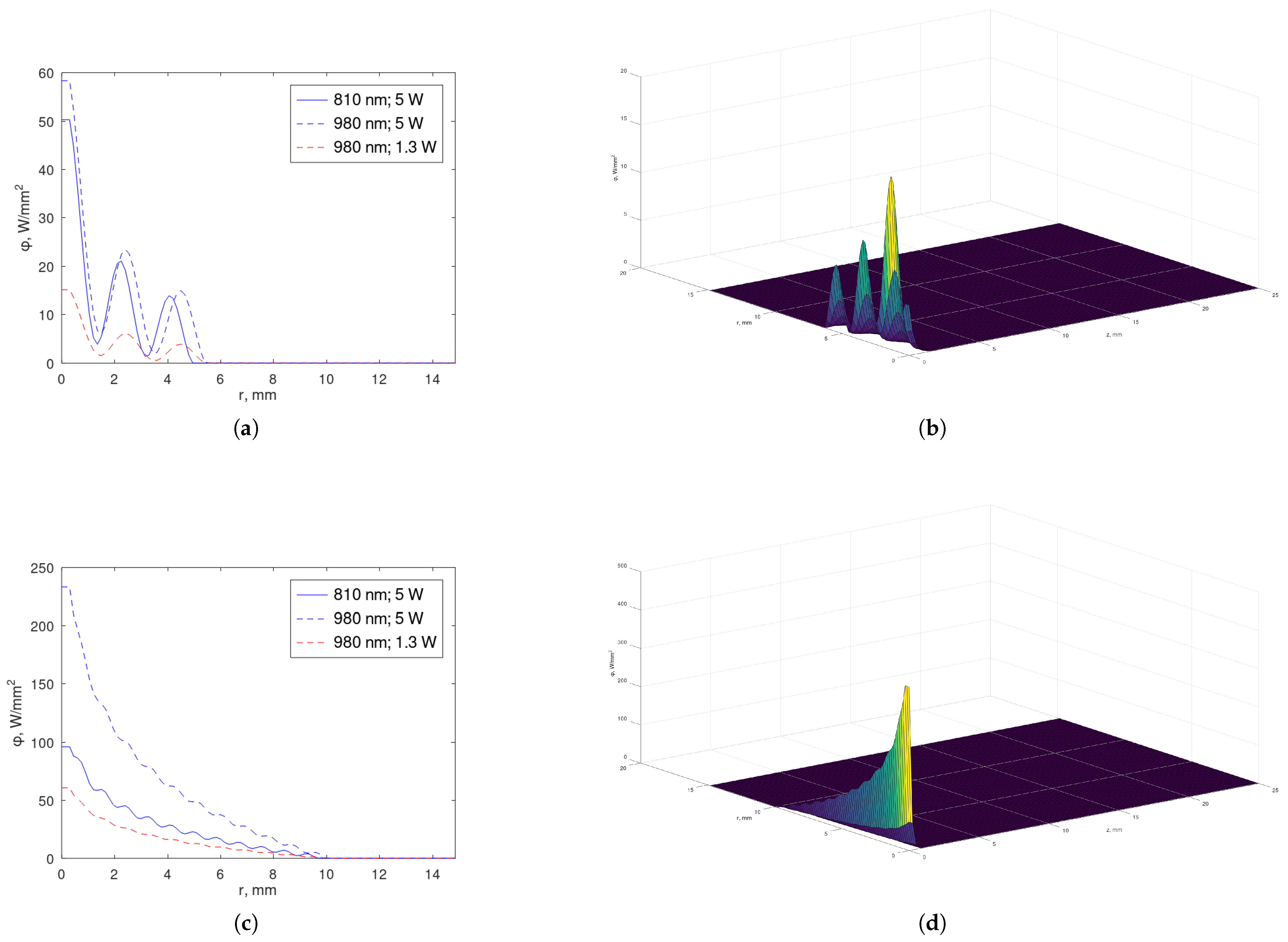
4.2. Profiles

In this study, we simulated results using the derived exact solution. The presented calculations were obtained using software GNU Octave version 7.2.0, under the optical parameters in Table 1.

Different wavelengths were used in this work to simulate two types of lasers: a Q-switched short-pulsed Nd:YAG laser operating at a wavelength of 1064 $\mathrm{n}$$\mathrm{m}$ and a diode short-pulsed laser operating at wavelengths of 810 $\mathrm{n}$$\mathrm{m}$ and 980 $\mathrm{n}$$\mathrm{m}$. Also, the values of the pulse widths vary. They can range from 500 ms to 2 ms in Nd:YAG lasers [16], from nanoseconds (1 $\mathrm{n}$$\mathrm{s}$ = $1\times {10}^{-9}$ $\mathrm{s}$) to picoseconds (1 $\mathrm{p}$$\mathrm{s}$ = $1\times {10}^{-12}$ $\mathrm{s}$) in most diode lasers, and are of femtosecond order (1 $\mathrm{f}$$\mathrm{s}$ = $1\times {10}^{-15}$ $\mathrm{s}$) in free-electron lasers.

We begin by analyzing the light absorption of the tissues according to the BL law. Figure 2 illustrates the linear and semi-log steady-state profiles of S for these operating wavelengths, under optical values of the carcinoma-adipose breast and tumor–healthy prostate tissues according to Table 1.

At the tip $z=0$, the source $S(0,0,t_p)$ has its maximum values according to

Table 2. Source values S [$\mathrm{W} {\mathrm{mm}}^{-3}$] at $z=0$ (maximum), and at the discontinuity $z=\ell$.

$\mathit{\lambda }$ [nm]	810	980	980	1064
${\mathit{P}}_{\mathbf{peak}}$ [W]	5	5	1.3	1.3
Maximum breast tumor	198	214	56	77
Minimum breast tumor	9.5 $\times {10}^{-28}$	6.8 $\times {10}^{-25}$	1.8 $\times {10}^{-25}$	3.9 $\times {10}^{-28}$
Maximum adipose breast	4.4 $\times {10}^{-42}$	6.3 $\times {10}^{-46}$	1.6 $\times {10}^{-46}$	3.1 $\times {10}^{-64}$
Maximum prostate tumor	647	828	215	420
Minimum prostate tumor	6.6 $\times {10}^{-62}$	2.2 $\times {10}^{-59}$	5.7 $\times {10}^{-60}$	2.7 $\times {10}^{-78}$
Maximum healthy prostate	2.6 $\times {10}^{-86}$	6.6 $\times {10}^{-100}$	1.7 $\times {10}^{-100}$	6.8 $\times {10}^{-200}$

. We emphasize that the source S does not exhibit expression in the outer region corresponding to the healthy tissue. The discontinuity of the source S, already mentioned in Section 4.1 [Case $0<t<t_p$], does not seem be addressed in the linear-scale graphical representations in (a) and (c) of Figure 2. Making recourse to the logarithmic scale for the y-direction, the discontinuity is clearly illustrated in (b) and (d) of Figure 2, whose minimum and maximum values are detailed in Table 2 for the tumor and healthy regions, respectively. Then, we may neglect the source S for $z>\ell$. For instance, at the power set at 5 $\mathrm{W}$ (in blue), with a wavelength of 810 $\mathrm{n}$$\mathrm{m}$ (solid line), we have $S(0,20,t_p)\simeq {10}^{-27} \mathrm{W} {\mathrm{mm}}^{-3}$ for the breast tumor border and $S(0,20,t_p)\simeq {10}^{-42} \mathrm{W} {\mathrm{mm}}^{-3}$ for the adipose breast border.

The fluence rate $\varphi$ has different graphical representations displayed in Figure 3, at diode pulse width $t_p=1\times {10}^{-11} \mathrm{s}$.

Figure 3 shows distributions of $\varphi$ for breast in (a) [$\mathrm{kW} {\mathrm{mm}}^{-2}$] and prostate in (c) [$\mathrm{TW} {\mathrm{mm}}^{-2}={10}^{12}\mathrm{W} {\mathrm{mm}}^{-2}$], as functions of the radius r, on different operating systems. Figure 3b shows distributions of $\varphi$ for breast for the power set at $1.3$ $\mathrm{W}$ and at a wavelength of 980 $\mathrm{n}$$\mathrm{m}$, corresponding to the red dashed line in (a). Figure 3d shows distributions of $\varphi$ for prostate for the power set at 5 $\mathrm{W}$ and at a wavelength of 810 $\mathrm{n}$$\mathrm{m}$, corresponding to the blue solid line in (b). At the referred values of pulse width in the order of $\mathrm{m}\mathrm{s}$ for Nd:YAG, the fluence rate $\varphi$ does not fit a coherent result. Indeed, the value of $exp\left[{\zeta }_{\mathrm{in}}{t}_p\right]\gg {10}^{+304}$. This drawback is due to the presence of the light velocity $\nu$ in the tissue.

Next, Figure 4 displays graphical representations of the fluence rate $\varphi$, at diode pulse width $t_p=1.0\mathrm{p}\mathrm{s}$. Figure 4 shows distributions of $\varphi$ for breast in (a) and prostate in (c), as functions of the radius r, on different operating systems. Again, the result relative to the situation of a wavelength of 1064 $\mathrm{n}$$\mathrm{m}$ is excluded for the same reason as before. Figure 4b and Figure 4d show distributions of $\varphi$ for breast and prostate, respectively, for the power set at $1.3$ $\mathrm{W}$ and at a wavelength of 980 $\mathrm{n}$$\mathrm{m}$, corresponding to the red dashed line in (a) and (b).

At the temporal pulse width $t_p$, the fluence rate does not rapidly decrease with distance from the tip surface, which implies that the Joule effect of heating is generated along the r-direction. Also, in Figure 4b,d, the slopes of curves in the z-direction illustrate that the fluence rate $\varphi$ is locally concentrated on the origin relative to the tip surface. The distributions of the fluence rate over time until $t_{\mathrm{end}}$ are the subject of study in forthcoming work. The analysis of the behavior of the outer radius $r_{\mathrm{o}}$ is still an open problem.

4.3. Temperature T and Tissue Damage

The time-dependent parameter $\zeta$ in (17) is

$$\zeta (\beta ;t)={\left(\rho c_{\mathrm{p}}\right)}^{-1}\left(k(\beta +{\mu }_{\mathrm{t}}^2)-c_{\mathrm{b}}{\rho }_{\mathrm{b}}w(1-t/t_{\mathrm{crit}})\right).$$

We set

$${\zeta }_1(\beta ;t)=\left\{\begin{array}{cc}\zeta (\beta ;0)\hfill & \mathrm{for} t<t_p\hfill \\ \zeta (\beta ;t)\hfill & \mathrm{for} t_p\le t<t_{\mathrm{crit}}\hfill \\ \zeta (\beta ;t_{\mathrm{crit}})\hfill & \mathrm{for} t\ge t_{\mathrm{crit}}\hfill \end{array}\right.$$

under parameter $\beta$, namely $\beta =0$, $\beta ={\beta }_1$, or $\beta ={\beta }_2$, according to Appendix A and Appendix B. Notice that $\zeta$ increases as a function of time and ${\zeta }_1$ obeys $\zeta (\beta ;0)\le {\zeta }_1(\beta ,t)\le \zeta (\beta ;t_{\mathrm{crit}})$ for all $t>0$. For the sake of simplicity, we write the constant ${\zeta }_0=\zeta (0;0)$. According to

Table 3. Average thermal parameters for blood and for breast and prostate (tumor and healthy) tissues [15,36].

	Unit	Blood	Breast Tumor	Prostate Tumor	Gland	Fatty Tissue
$\rho$	$\mathrm{kg} {\mathrm{m}}^{-3}$	1060.00	1000.00	999.00	1041.00	920.00
${\omega }_0$	$\mathrm{kg} {\mathrm{m}}^{-3}{\mathrm{s}}^{-1}$		0.5	0.416	0.54	0.32

, we can calculate ${\zeta }_0$ in the tumors (cf.

Table 4. Values for parameter ${\zeta }_0$ at different wavelengths.

$\mathit{\lambda }$ [nm]	Breast	Prostate
810	1.7 $\times {10}^3$	7.9 $\times {10}^3$
980	1.4 $\times {10}^3$	7.3 $\times {10}^3$
1064	1.7 $\times {10}^3$	1.2 $\times {10}^4$

).

The breast tumor is commonly located in the gland tissue. If the breast tumor is located in the adipose tissue, the healthy tissue will exhibit lower density and blood perfusion values than those of the tumor for the prostate values (cf. Table 3). Also, the density of any tumor varies from lower values at a primary stage to very high values.

Thanks to the Duhamel principle (for details, see [31]), the solution of (8) and (9) is, for $0\le r\le r_{\mathrm{f}}$ and $0\le z\le \ell$, as follows:

• If $0\le t<t_p$,

  $$\begin{array}{cc}\hfill T(r,z,t)& =T_{\mathrm{b}}+{\displaystyle \frac{{\mu }_{\mathrm{a}}}{\rho c_{\mathrm{p}}}}{\displaystyle \frac{S(r_{\mathrm{f}},z,0)}{D{\mu }_{\mathrm{t}}^2-{\mu }_{\mathrm{a}}}}{\int }_0^t\left(exp\left[{\zeta }_{\mathrm{in}}s\right]-1\right)exp\left[{\zeta }_0(t-s)\right]s\hfill \\ \hfill & =T_{\mathrm{b}}+{\mu }_{\mathrm{a}}{S}_{\mathrm{in}}exp[-{\mu }_{\mathrm{t}}z]\left({\displaystyle \frac{exp\left[{\zeta }_{\mathrm{in}}t\right]-exp\left[{\zeta }_{0}t\right]}{\rho c_{\mathrm{p}}({\zeta }_{\mathrm{in}}-{\zeta }_0)}}+{\displaystyle \frac{1-exp\left[{\zeta }_{0}t\right]}{k{\mu }_{\mathrm{t}}^2-c_{\mathrm{b}}{\rho }_{\mathrm{b}}w}}\right);\hfill \end{array}$$
• If $t\ge t_p$,

  $$T(r,z,t)=T(r_{\mathrm{f}},z,t_p)+{\displaystyle \frac{{\mu }_{\mathrm{a}}}{c_{\mathrm{p}}\rho }}{\int }_{t_p}^t\varphi (r_{\mathrm{f}},z,s)exp\left[{\int }_0^{t-s}{\zeta }_1(0;\tau )\tau \right]s.$$

We may extend the temperature T to the entire multidomain by proceeding as in Section 4.1.

To evaluate the thermal damage, we need to estimate $t_{\mathrm{crit}}$. From (10), we have

$${\displaystyle \frac{1}{A}}exp\left[{\displaystyle \frac{E_{\mathrm{a}}}{R{T}_{\max }}}\right]\le t_{\mathrm{crit}}\le {\displaystyle \frac{1}{A}}exp\left[{\displaystyle \frac{E_{\mathrm{a}}}{R{T}_{\min }}}\right],$$

(25)

where

$$T_{\max }=\underset{\mathrm{\Omega }\times ]0;t_{\mathrm{crit}}[}{sup}T;T_{\min }=\underset{\mathrm{\Omega }\times ]0;t_{\mathrm{crit}}[}{inf}T.$$

The minimum temperature $T_{\min }=T_{\mathrm{b}}$ and $t_{\mathrm{crit}}$ obeying (25) verify

$$t_{\mathrm{crit}}\le {\displaystyle \frac{1}{A}}exp\left[{\displaystyle \frac{E_{\mathrm{a}}}{R{T}_{\mathrm{b}}}}\right].$$

(26)

Typical values for prostate tumor are $E_{\mathrm{a}}=5.67\times {10}^5 \mathrm{J} {mol}^{-1}$ and $A=1.7\times {10}^{91} {\mathrm{s}}^{-1}$ [5]. Based on these values, (26) implies that $t_{\mathrm{crit}}$ obeys the upper bound $t_{\mathrm{crit}}\le 9.9\times {10}^3\mathrm{s}\sim 2.75 \mathrm{h}$. As commonly accepted, the maximum temperature with respect to produce complete in situ destruction of tissue is $T_{\max }=50$°C. Then, $t_{\mathrm{crit}}$ similarly obeys the lower bound $t_{\mathrm{crit}}\ge 2.8871\mathrm{s}$.

5. Discussion

We firstly emphasize that the validity of the diffusion approximation of the radiative transfer equation, namely Equation (1), is true. Some important findings include the fact that the criterion ${\mu }_{\mathrm{a}}\ll {\mu }_{\mathrm{s}}^{\prime }$ cannot be disregarded in the validity of the stationary diffusion approximation, as stated but not proven in [21] for any geometric domain: plane ([21], Section 6.4.1), spherical with an isotropic point source ([21], Section 6.4.2), or cylindrical ([21], Section 6.4.3). The criterion ${\mu }_{\mathrm{a}}\ll {\mu }_{\mathrm{s}}^{\prime }$ in the validity is precisely quantified in [39] as ${\mu }_{\mathrm{a}}/{\mu }_{\mathrm{s}}^{\prime }\sim 1/100$. According to Table 1, we calculated ${\mu }_{\mathrm{a}}/{\mu }_{\mathrm{s}}^{\prime }$ (cf.

Table 5. Values for ${\mu }_{\mathrm{a}}/{\mu }_{\mathrm{s}}^{\prime }$ at different wavelengths.

$\mathit{\lambda }$ [nm]	Breast Tumor	Breast Tissue	Prostate Tumor	Prostate Tissue
810	7.9 × ${10}^{-3}$	1.7 × ${10}^{-2}$	8.2 × ${10}^{-3}$	4.2 × ${10}^{-2}$
980	9.2 × ${10}^{-3}$	2.4 × ${10}^{-2}$	1.0 × ${10}^{-2}$	4.7 × ${10}^{-2}$
1064	8.9 × ${10}^{-3}$	4.0 × ${10}^{-2}$	1.1 × ${10}^{-2}$	4.3 × ${10}^{-2}$

).

The criterion is verified by all values. Although some of the values are indeed greater, they verify ${\mu }_{\mathrm{a}}/{\mu }_{\mathrm{s}}^{\prime }\sim 1/100$. In contrast, in [46], the authors argue that the $\delta$-Eddington approximation to the Boltzmann transport equation provides a small percentage error if ${\mu }_{\mathrm{s}}^{\prime }/{\mu }_{\mathrm{a}}\sim 100$.

Our first finding is that the source S does not reach the outer region correspondent to the healthy tissue when the laser emission tip surface is located at the middle of the tumor for one pulse width. Figure 2 and Table 2 confirm the local behavior of the source S. Its longitudinal discontinuity, shown in Figure 2b,d, is a consequence of the tissue dependence on the optical values.

Relationship (17) implies other conclusions regarding the diffusion approximation of the radiative transfer equation. If the source of the scattered photons S is given as a function of the effective attenuation coefficient ${\mu }_{\mathrm{eff}}=\sqrt{3{\mu }_{\mathrm{a}}({\mu }_{\mathrm{a}}+{\mu }_{\mathrm{s}}^{\prime })}$ [23], then relationship (17) reads $\zeta /\nu +{\mu }_{\mathrm{a}}=D{\mu }_{\mathrm{eff}}^2={\mu }_{\mathrm{a}}$. This means that the fluence rate will be in steady state because $\zeta =0$. In [37], the author presents a detailed analytical solution of the diffuse radiant fluence rate for the time-independent searchlight problem on flat-slab and semi-infinite geometries, under homogeneous Dirichlet conditions, using Green’s function method. Also, the author refers to some inaccuracies of the diffusion approximation.

In Section 4.1, we derive the fluence rate $\varphi$ as a solution of (1). Its simulations, throughout the inlet region, originated by the tumor, and the outlet region, originated by the healthy tissue, are illustrated in Figure 3 and Figure 4, with different pulse widths.

On the one hand, we observe that different behaviors occur at different pulse width values by comparing Figure 3 and Figure 4, which suggests that there are values of the pulse width that blow up the exponential function, namely at pulse widths $t_p=10 \mathrm{p}\mathrm{s}$ or above. Thus, the proposed exact solutions for the mathematical model may be a tool for FLA under diode lasers. However, they do not cover Nd:YAG lasers.

On the other hand, the present results in Figure 4a,c suggest that power alone is a stronger contributor of the profile magnitude than wavelengths. We observe that Figure 3c for the prostate tissue indicates the wavelength of the main contributor of the profile magnitude. However, taking into account the previous comment about the comparison between Figure 3 and Figure 4, we discard the last observation in order to avoid ambiguities and erroneous conclusions.

Moreover, we observe different oscillating patterns in the decreasing behavior of the fluence rate on the breast and prostate tissues. The simulation results in Figure 4 illustrate that the radial distribution has an oscillating pattern with a smaller amplitude and frequency in (c) and (d), correspondent to the prostate tissue, than in (a) and (b), correspondent to the breast tissue. This means that the configurations of the physical problem solved may differ in the presence of any perturbation on the data. In the cancer–laser literature, as mentioned in the Introduction section, experimental studies and numerical analyses have been focused on the temperature response to a given heat source. This source indeed varies, among radiofrequency, microwave, cryoablation, ultrasound, and laser techniques. The present work found new analytical solutions for a coupled PDE system modeling light penetration and heat transfer in biological tissues during focal laser ablation. As far as we know, the simulated results from the derived solutions are new, and their potential physical contributions are still open problems.

Evaluating the critical time $t_{\mathrm{crit}}$, as defined in Section 4.3 by Arrhenius burn integration (10), is based on the dependence of parameters A or $E_a$. A breaking point for either A or $E_a$ is reported in [47], at $T=54$ °C, which is greater than 50 °C (known as the maximum temperature with respect to producing complete in situ destruction of tissue). To produce the complete cure of the patient at the shortest treatment time (for instance, $t_{\mathrm{crit}}=2.8871 \mathrm{s}$ for prostate tumor) is the desired objective.

The various equations in the present paper allow us to calculate the light fluence rate as a function of $(r,z,t)$, within different regions in space. We apply them to breast and prostate tumors, but they may be applied to any tumor kind, based on the optical and thermal properties of the tissue under study. According to the experimental methods, we set higher optical values for the tumor tissue than for the healthy tissue, but our results may be replicated with inverse optical values. Finally, the optical parameters were assumed to be wavelength-dependent but temperature-independent according to [24,25,35,38]. We emphasize that the temperature is a function on the space–time coordinate system, which solves the Pennes bioheat transfer Equation (8). On the one hand, if the coefficients are space–time-dependent, they invalidate the application of the separable variable method. On the other hand, the coupled PDE system, (1) and (8), is nonlinear, and then we can only split it by considering a fixed point argument.

6. Conclusions

To study the heat exchange problem for ablation performed in biomedical sciences, it is important to precisely analyze its source, the absorbed optical power density (9). The derived solution might be a tool with which to generate quantitative and/or qualitative results. We detail their derivation to allow their application to various tumors through adjusting for their optical and thermal properties.

Our conclusions are the following:

• Although the validity of the diffusion approximation of the radiative transfer equation is achieved under the criteron ${\mu }_{\mathrm{a}}/{\mu }_{\mathrm{s}}^{\prime }\sim 1/100$, the exact solution for the fluence rate depends on the choice of the pulse width. Different pulse widths affect the fluence rate, with significant changes observed at pulse widths of 10 ps or more. This emphasizes the importance of diffusion approximation and the unsteady-state fluence rate, contributing to the understanding of biothermophysical problems.
• If the laser tip is fixed at the center of the tumor, its action is local. Then, a moving tip, as used in EVLA [31], should be the object of study in future research in order to find out if a better performance will be provided.
• The exact solutions are of the exponential type as functions of time. The increasing behavior during the temporal pulse width has greater contribution than the decreasing behavior during the subsequent period (the pulse-to-pulse interval). At pulse widths of order $\mathrm{p}\mathrm{s}$, we may conclude that a further study of the time-dependent searchlight problem is a priority.
• The treatment should have a moving focal point with a short exposure time $t_{\mathrm{end}}=t_{\mathrm{crit}}$ to preserve the healthy tissue.

References

1. Voeller, R.K.; Schuessler, R.B.; Damiano, R.J., Jr. Surgical Treatment of Atrial Fibrillation. In Cardiac Surgery in the Adult; Lh, C., Ed.; McGraw-Hill: New York, NY, USA, 2008; Chapter 59; pp. 1375–1394. [Google Scholar]
2. Fan, Y.; Xu, L.; Liu, S.; Li, J.; Xia, J.; Qin, X.; Li, Y.; Gao, T.; Tang, X. The state-of-the-art and perspectives of Laser Ablation for tumor treatment. Cyborg Bionic Syst. 2024, 5, 0062. [Google Scholar] [CrossRef] [PubMed]
3. Loiola, B.R.; Orlande, H.R.B.; Dulikravich, G.S. Thermal damage during ablation of biological tissues. Numer. Heat Transf. Part A Appl. 2018, 73, 685–701. [Google Scholar] [CrossRef]
4. Lazarovich, A.; Viswanath, V.; Dahmen, A.S.; Sidana, A. A narrative clinical trials review in the realm of focal therapy for localized prostate cancer. Transl. Cancer Res. 2024, 13, 6529–6539. [Google Scholar] [CrossRef] [PubMed]
5. He, X.; Bischof, J. Quantification of temperature and injury response in thermal therapy and cryosurgery. Crit. Rev. Biomed. Eng. 2003, 31, 355–421. [Google Scholar] [CrossRef]
6. Consiglieri, L.; dos Santos, I.; Haemmerich, D. Theoretical analysis of the heat convection coefficient in large vessels and the significance for thermal ablative therapies. Phys. Med. Biol. 2003, 48, 4125–4134. [Google Scholar] [CrossRef]
7. Consiglieri, L. Continuum models for the cooling effect of blood flow on thermal ablation techniques. Int. J. Thermophys. 2012, 33, 864–884. [Google Scholar] [CrossRef]
8. Pupo, A.; González, M.; Cabrales, L.; Reys, J.; Oria, E.; Nava, J.; Jiménez, R.; Sanchéz, F.; Ciria, H.; Cabrales, J. 3d current density in tumors and surrounding healthy tissues generated by a system of straight electrode arrays. Math. Comput. Simul. 2017, 138, 49–64. [Google Scholar] [CrossRef]
9. González-Suárez, A.; Pérez, J.J.; Irastorza, R.M.; D’Avila, A.; Berjano, E. Computer modeling of radiofrequency cardiac ablation: 30 years of bioengineering research. Comput. Methods Programs Biomed. 2022, 214, 106546. [Google Scholar] [CrossRef]
10. Chiang, J.; Birla, S.; Bedoya, M.; Jones, D.; Subbiah, J.; Brace, C.L. Modeling and validation of microwave ablations with internal vaporization. IEEE Trans. Biomed. Eng. 2015, 62, 657–663. [Google Scholar] [CrossRef]
11. Wang, J.; Wu, S.; Wu, Z.; Gao, H.; Huang, S. Influences of blood flow parameters on temperature distribution during liver tumor microwave ablation. Front. Biosci.-Landmark 2021, 26, 504–516. [Google Scholar] [CrossRef]
12. Franco, W.; Liu, J.; Wang, G.X.; Nelson, J.S.; Aguilar, G. Radial and temporal variations in surface heat transfer during cryogen spray cooling. Phys. Med. Biol. 2005, 50, 387. [Google Scholar] [CrossRef] [PubMed]
13. Boronyak, S.M.; Merryman, W.D. Development of a simultaneous cryo-anchoring and radiofrequency ablation catheter for percutaneous treatment of mitral valve prolapse. Ann. Biomed. Eng. 2012, 40, 1971–1981. [Google Scholar] [CrossRef] [PubMed]
14. Kumar, M.; Rai, K.N. Three phase bio-heat transfer model in three-dimensional space for multiprobe cryosurgery. J. Therm. Anal. Calorim. 2022, 147, 14491–14507. [Google Scholar] [CrossRef]
15. Ho, C.S.; Ju, K.C.; Cheng, T.Y.; Chen, Y.Y.; Lin, W.L. Thermal therapy for breast tumors by using a cylindrical ultrasound phased array with multifocus pattern scanning: A preliminary numerical study. Phys. Med. Biol. 2007, 52, 4585–4599. [Google Scholar] [CrossRef]
16. Mordon, S.; Buys, B.; Brunetaud, J.; Moschetto, Y. New directions in medical laser concept: Role of laser-tissue interaction modelization and feedback control. Lasers Med. Sci. 1989, 4, 317–327. [Google Scholar] [CrossRef]
17. Vogel, A.; Venugopalan, V. Pulsed Laser Ablation of Soft Biological Tissues. In Optical-Thermal Response of Laser-Irradiated Tissue; Welch, A.J., van Gemert, M.J., Eds.; Springer Science+Business Media B.V.: Dordrecht, The Netherlands, 2011; Chapter 14; pp. 551–615. [Google Scholar] [CrossRef]
18. Putzer, M.; Rogério da Silva, G.; Michael, K.; Schröder, N.; Schudeleit, T.; Bambach, M.; Wegener, K. Geometrical modeling of ultrashort pulse laser ablation with redeposition and analysis of the influence of spot size and shape. Mater. Des. 2024, 246, 113357. [Google Scholar] [CrossRef]
19. Vita, E.D.; Landro, M.D.; Massaroni, C.; Iadicicco, A.; Saccomandi, P.; Schena, E.; Campopiano, S. Fiber optic sensors-based thermal analysis of perfusion-mediated tissue cooling in liver undergoing laser ablation. IEEE Trans. Biomed. Eng. 2021, 68, 1066–1073. [Google Scholar] [CrossRef]
20. Schena, E.; Saccomandi, P.; Fong, Y. Laser Ablation for cancer: Past, Present and Future. J. Funct. Biomater. 2017, 8, 19. [Google Scholar] [CrossRef]
21. Star, W.M. Diffusion Theory of Light Transport. In Optical-Thermal Response of Laser-Irradiated Tissue; Welch, A.J., van Gemert, M.J., Eds.; Springer: New York, NY, USA, 1995; Chapter 6; pp. 131–206. [Google Scholar]
22. Liu, H.; Boas, D.; Zhang, Y.; Yodh, A.; Chance, B. Determination of optical properties and blood oxygenation in tissue using continuous NIR light. Phys. Med. Biol. 1995, 40, 1983–1993. [Google Scholar] [CrossRef]
23. Oden, J.T.; Diller, K.R.; Bajaj, C.; Browne, J.C.; Hazle, J.; Babuška, I.; Bass, J.; Biduat, L.; Demkowicz, L.; Elliott, A.; et al. Dynamic data-driven finite element models for laser treatment of cancer. Numer. Methods Partial Differ. Equ. 2007, 23, 904–922. [Google Scholar] [CrossRef]
24. Sandell, J.L.; Zhu, T.C. A review of in-vivo optical properties of human tissues and its impact on PDT. J. Biophotonics 2011, 4, 773–787. [Google Scholar] [CrossRef] [PubMed]
25. Whiting, P.; Dowden, J.; Kapadia, P.; Davis, M. A one-dimensional mathematical model of laser induced thermal ablation of biological tissue. Lasers Med. Sci. 1992, 7, 357–368. [Google Scholar] [CrossRef]
26. Durkee, J.J.; Antich, P.; Lee, C. Exact solutions to the multiregion time-dependent bioheat equation. I: Solution development. Phys. Med. Biol. 1990, 35, 847–867. [Google Scholar] [CrossRef]
27. Consiglieri, L. An analytical solution for a bio-heat transfer problem. Int. J. Bio-Sci. Bio-Technol. 2013, 5, 267–278. [Google Scholar] [CrossRef]
28. Consiglieri, L. Analytical solutions in the modeling of the local RF ablation. J. Mech. Med. Biol. 2016, 16, 1650071. [Google Scholar] [CrossRef]
29. Liu, J.; Chen, X.; Xu, L. New thermal wave aspects on burn evaluation of skin subjected to instantaneous heating. IEEE Trans. Biomed. Eng. 1999, 46, 420–428. [Google Scholar]
30. Paul, A.; Bandaru, N.; Narasimhan, A.; Das, S. Subsurface tumor ablation with near-infrared radiation using intratumoral and intravenous injection of nanoparticles. Int. J. Micro-Nano Scale Transp. 2014, 5, 69–80. [Google Scholar] [CrossRef]
31. Consiglieri, L. Analytical solutions in the modelling of the endovenous laser ablation. Rev. Acad. Colomb. Cienc. Exactas Fis. Nat. 2024, 48, 254–270. [Google Scholar] [CrossRef]
32. Banerjee, A.; Ogale, A.; Das, C.; Mitra, K.; Subramanian, C. Temperature distribution in different materials due to short pulse laser irradiation. Heat Transfer Eng. 2005, 26, 41–49. [Google Scholar] [CrossRef]
33. D’Alessandro, G.; Tavakolian, P.; Sfarra, S. A review of techniques and bio-heat transfer models supporting infrared thermal imaging for diagnosis of malignancy. Appl. Sci. 2024, 14, 1603. [Google Scholar] [CrossRef]
34. Manenti, G.; Perretta, T.; Nezzo, M.; Fraioli, F.; Carreri, B.; Gigliotti, P.; Micillo, A.; Malizia, A.; Di Giovanni, D.; Ryan, C.; et al. Transperineal Laser Ablation (TPLA) treatment of focal low-intermediate risk prostate cancer. Cancers 2024, 16, 1404. [Google Scholar] [CrossRef] [PubMed]
35. Niemz, M. Laser-Tissue Interactions: Fundamentals and Applications; Springer: Berlin/Heidelberg, Germany, 2007. [Google Scholar]
36. Marqa, M.F.; Colli, P.; Nevoux, P.; Mordon, S.; Betrouni, N. Focal Laser Ablation of prostate cancer: Numerical simulation of temperature and damage distribution. BioMed. Eng. OnLine 2011, 10, 45. [Google Scholar] [CrossRef] [PubMed]
37. Prahl, S.A. The diffusion approximation in three dimensions. In Optical-Thermal Response of Laser-Irradiated Tissue; Welch, A.J., Van Gemert, M.J.C., Eds.; Springer: New York, NY, USA, 1995; Chapter 7; pp. 207–231. [Google Scholar]
38. Jacques, S. Optical properties of biological tissues: A review. Phys. Med. Biol. 2013, 58, R37–R61. [Google Scholar] [CrossRef] [PubMed]
39. Capart, A.; Ikegaya, S.; Okada, E.; Machida, M.; Hoshi, Y. Experimental tests of indicators for the degree of validness of the diffusion approximation. J. Phys. Commun. 2021, 5, 025012. [Google Scholar] [CrossRef]
40. Rylander, M.; Feng, Y.; Bass, J.; Diller, K. Thermally induced injury and heat shock protein expression in cells and tissues. Ann. N. Y. Acad. Sci. 2005, 1066, 222–242. [Google Scholar] [CrossRef]
41. Guo, Z.; Kim, K. Ultrafast laser radiation transfer in heterogeneous tissues with the discrete ordinate method. Appl. Opt. 2003, 42, 2897–2905. [Google Scholar] [CrossRef]
42. Jaunich, M.; Raje, S.; Kim, K.; Mitra, K.; Guo, Z. Bio-heat transfer analysis during short pulse laser irradiation of tissues. Int. J. Heat Mass Transfer 2008, 51, 5511–5521. [Google Scholar] [CrossRef]
43. Tang, D.; Araki, N. On non-Fourier temperature wave and thermal relaxation time. Int. J. Thermophys. 1997, 18, 493–504. [Google Scholar] [CrossRef]
44. Dutta, J.; Kundu, B. An improved analytical model for heat flow in cancerous tumours to avoid thermal injuries during hyperthermia. Proc. Inst. Mech. Eng. Part H J. Eng. Med. 2021, 235, 500–514. [Google Scholar] [CrossRef]
45. Özisik, M. Heat Conduction; John Wiley & Sons, Ltd.: New York, NY, USA, 2012. [Google Scholar]
46. Carp, S.; Prahl, S.; Venugopalan, V. Radiative transport in the delta-P1 approximation: Accuracy of fluence rate and optical penetration depth predictions in turbid semi-infinite media. J. Biomed. Opt. 2004, 9, 632–647. [Google Scholar] [CrossRef]
47. Rylander, M.; Feng, Y.; Zimmermann, K.; Diller, K. Measurement and mathematical modeling of thermally induced injury and heat shock protein expression kinetics in normal and cancerous prostate cells. Int. J. Hyperthermia 2010, 26, 748–764. [Google Scholar] [CrossRef]
48. Olver, F. Bessel functions of integer order. In Handbook of Mathematical Functions with Formulas, Graphs, and Mathematical Tables; Abramonitz, M., Stegun, I., Eds.; United States Department of Commerce: Washington, DC, USA, 1972; Chapter 9; pp. 355–389. [Google Scholar]
Figure 1. Schematic representations of the laser–tissue system: the laser emission tip Γ tip = { ( x , y ) R 2 : x 2 + y 2 < r f 2 } × { 0 } , the light-emitting cylinder ] 0 ; r f [ × ] 0 ; L [ , the tumor Ω i = ] 0 ; r i [ × ] ; [ , and the surrounding healthy tissue Ω o = { ( x , y ) R 2 : x 2 + y 2 < r i 2 } × ] ; L [ { ( x , y ) R 2 : r i 2 < x 2 + y 2 < r o 2 } × ] 0 ; L [ . (Left) Sagittal view. (Right) Cylindrical coordinates ( r , z ) .
Photonics 12 00400 g001
Figure 2. Graphical representations of the source S [ W   mm 3 ] at different wavelengths and power sets. (a) Plot with linear axes of the breast source. (b) Plot using a logarithmic scale for the y-axis of the breast source. (c) Linear plot of the prostate source. (d) Semilog plot of the prostate source. For details, see Table 2.
Photonics 12 00400 g002
Figure 3. (a) Breast radial graphical representations of the fluence rate ϕ [ kW   mm 2 ] at different wavelengths and power sets. (b) Plot of the fluence rate ϕ [ kW   mm 2 ] for the tumor-adipose breast tissue at the wavelength of 980  n m and power set at 1.3   W . (c) Prostate radial graphical representations of the fluence rate ϕ [ TW   mm 2 ] at different wavelengths and power sets. (d) Plot of the fluence rate ϕ [ TW   mm 2 ] for the tumor–healthy prostate tissue at the wavelength of 810  n m and power set at 5  W .
Photonics 12 00400 g003
Figure 4. (a) Breast radial graphical representations of the fluence rate ϕ at different wavelengths and power sets. (b) Plot of the fluence rate ϕ for the tumor-adipose breast tissue at the wavelength of 980  n m and power set at 1.3   W . (c) Prostate radial graphical representations of the fluence rate ϕ at different wavelengths and power sets. (d) Plot of the fluence rate ϕ for the tumor–healthy prostate tissue at the wavelength of 980  n m and power set at 1.3   W .
Photonics 12 00400 g004