Metasurface-Refractive Hybrid Lens Modeling with Vector Field Physical Optics

Abstract

Metasurfaces (MSs) have emerged as a promising technology for optical system design. When combined with traditional refractive optics, MS-refractive hybrid lenses can enhance imaging performance, reduce optical aberrations, and introduce new functionalities such as polarization control. However, modeling these hybrid lenses requires advanced simulation techniques that usually go beyond conventional raytracing tools. This work presents a physical optics framework for modeling MS-refractive hybrid lenses. We introduce a ray-wave hybrid method that integrates multiple propagation techniques to account for vector wave propagation through various optical elements. At the center of the proposed framework is the Gaussian decomposition method for modeling beam propagation through refractive optics. Ray-path diffraction is automatically considered in this method, and complex input wavefront can be modeled as well. Several techniques are integrated to ensure accuracy in decomposing an incoming vector wave into Gaussian beamlets, such as adaptive consideration of local wavefront principal curvatures and best-fit beam width estimation from the local covariance matrix. To demonstrate the effectiveness of our method, we apply it to several hybrid lens designs, including polarization-sensitive MSs and aberration-correcting MSs integrated into complex optical systems.

1. Introduction

Metasurfaces (MSs) are flat optics providing flexible phase, amplitude, and polarization control by engineering the nano-structure of each meta-atom. Leveraging these unique properties, MSs have been utilized to address achromatic lenses [1,2,3,4], to enable polarization control or conversion [5,6,7,8], to realize multifunctional imaging [9,10,11,12], and even to be integrated with optoelectronic devices for on-chip light control [13,14]. Meanwhile, the integration of MSs with conventional refractive optics has led to novel lens designs, enabling the creation of MS-refractive hybrid lenses with enhanced versatility and functionality, particularly in applications demanding compact form factors and multi-functional lenses [15,16,17,18,19,20].

In the design of MS-refractive hybrid lenses, simulating imaging performance is a critical step. However, achieving a rigorous solution by electromagnetic field solvers poses substantial computational challenges, particularly for lenses with large apertures. This scale disparity between the meta-atom subwavelength features and the macroscopic lens aperture typically renders rigorous solvers impractical due to their high computational cost. Consequently, designers often rely on approximations through raytracing tools or physical optics solvers to balance computational feasibility with model accuracy.

Commercial optical design software, such as Code V (11.5 SR1) and Zemax (2022 R2.02), can simulate MS-refractive hybrid lenses by incorporating customized surfaces or source models to approximate MS response. For instance, Cuillerier et al. proposed a semi-analytical model where the MS is represented as a user-defined phase surface, allowing the MS phase modulation properties to be incorporated within the raytracing framework [21]; Chen et al. introduced a method to model an MS as an effective refractive surface, taking the meta-atom dispersion relation into account to more accurately reflect wavelength-dependent behaviors, and can lead to broadband aberration correction with MSs [22]. These approaches facilitate the integration of MSs in traditional lens designs, leveraging the built-in optimization capabilities of the software. However, these models typically rely on approximations that may not fully capture complex polarization effects or detailed wave-based interactions, which are important for hybrid lenses with polarization-sensitive MSs. Further, while some commercial packages, such as VirtualLab Fusion and RSoft, incorporate advanced techniques to simulate MS behavior and propagation across refractive optics [23], the underlying algorithms are proprietary and not fully disclosed to the public, limiting users’ ability to customize or extend the methods to meet specific needs. In contrast, this work intends to provide a transparent approach for simulating polarization-sensitive propagation in MS-refractive hybrid lenses.

A ray-wave hybrid method introduced in Reference [24] can be used to simulate scalar field propagation in MS-refractive hybrid lenses, which demonstrated potential for the inverse design of aberration-correcting MSs. This approach employs the angular spectrum method (ASM) to model free-space propagation accurately. For the propagation of wavefronts through curved refractive elements, a ray-field method (RFM) is used to enable efficient raytracing. In that method, the MS was treated as a polarization-insensitive phase surface, simplifying the model to focus on phase modulation effects.

Despite its utility, this method modeled light fields as scalar waves, omitting polarization effects. Such an assumption may be inadequate, particularly for hybrid lenses with polarization-sensitive MSs, or refractive elements with anti-reflection coatings. Moreover, the simplified formalism of the RFM restricts its applicability: Since the RFM disregards ray path diffraction, it is unsuitable for accurately simulating wavefront propagation to a focal point or over long distances, where diffraction effects significantly alter the beam profile.

To address these limitations, this work extends the ray-wave hybrid method to incorporate polarization effects, allowing polarization tracking across multiple observation planes within a hybrid lens. In the proposed approach, the MS introduces local phase and amplitude modulations based on meta-atom responses under the local uniformity approximation (LUA). This permits the use of rigorous coupled-wave analysis (RCWA) to obtain local complex transmission coefficients, capturing the polarization dependence and angular response of each meta-atom. Free-space propagation continues to be managed by the ASM for a full-wave solution, while the Gaussian decomposition method (GDM) is introduced for field propagation through refractive optics. GDM is a more generalized approach than RFM, as it naturally incorporates ray path diffraction effects. The numerical implementation of GDM and its advantages over RFM will be a key focus of this work.

These extensions enable physical optics modeling of complex beam propagation within MS-refractive hybrid lenses, allowing exploration of their performance while maintaining computational efficiency. Several examples are presented to demonstrate the proposed method’s versatility, including hybrid lenses (1) having aberration-correcting MSs, (2) designed to focus cylindrically polarized beams, (3) incorporating multifunctional MSs developed through adjoint gradient design techniques, and (4) for full-Stokes polarization sensing.

2. Formalism

Physical optics modeling involves propagating optical waves sequentially from a source through complex systems including several types of optical components. Referring to Figure 1, in the context of MS-refractive hybrid systems, appropriate physical optics propagators are essential to account for the distinct behaviors of different components. These propagators must manage: (1) the local phase and amplitude modulation imposed by MSs, (2) propagation through refractive optics with curved surfaces, and (3) transmission through the homogeneous media that connect these elements.

Table 1. Comparison of physical optics propagators for MS-refractive hybrid systems.

Method	Speed	Application Scope	Accuracy	Strengths	Limitations
ASM	Fast	Free-space	High	Provides full-wave solution for free-space propagation	Limited to homogeneous, non-refractive media
GDM	Moderate	Refractive optics and free-space	High	Captures diffraction effects, handles non-paraxial propagation	Slower than RFM; requires careful decomposition strategy
RFM	Very fast	Refractive optics and free-space	Moderate	Efficient for large-scale simulations; works well for smooth wavefronts	Cannot handle diffraction effects; inaccurate near foci or caustics
RCWA	Moderate	Nanostructured surfaces (e.g., MS) under the LUA	High for slow-varying structures	Efficiently models MS response including polarization and angular dependence	Limited to slow-varying MS; computationally expensive for large surfaces

provides a concise comparison of the physical optics propagators used in this work, outlining their applicability, accuracy, and computational efficiency in modeling MS-refractive hybrid systems. The following subsections provide a more detailed discussion of each method.

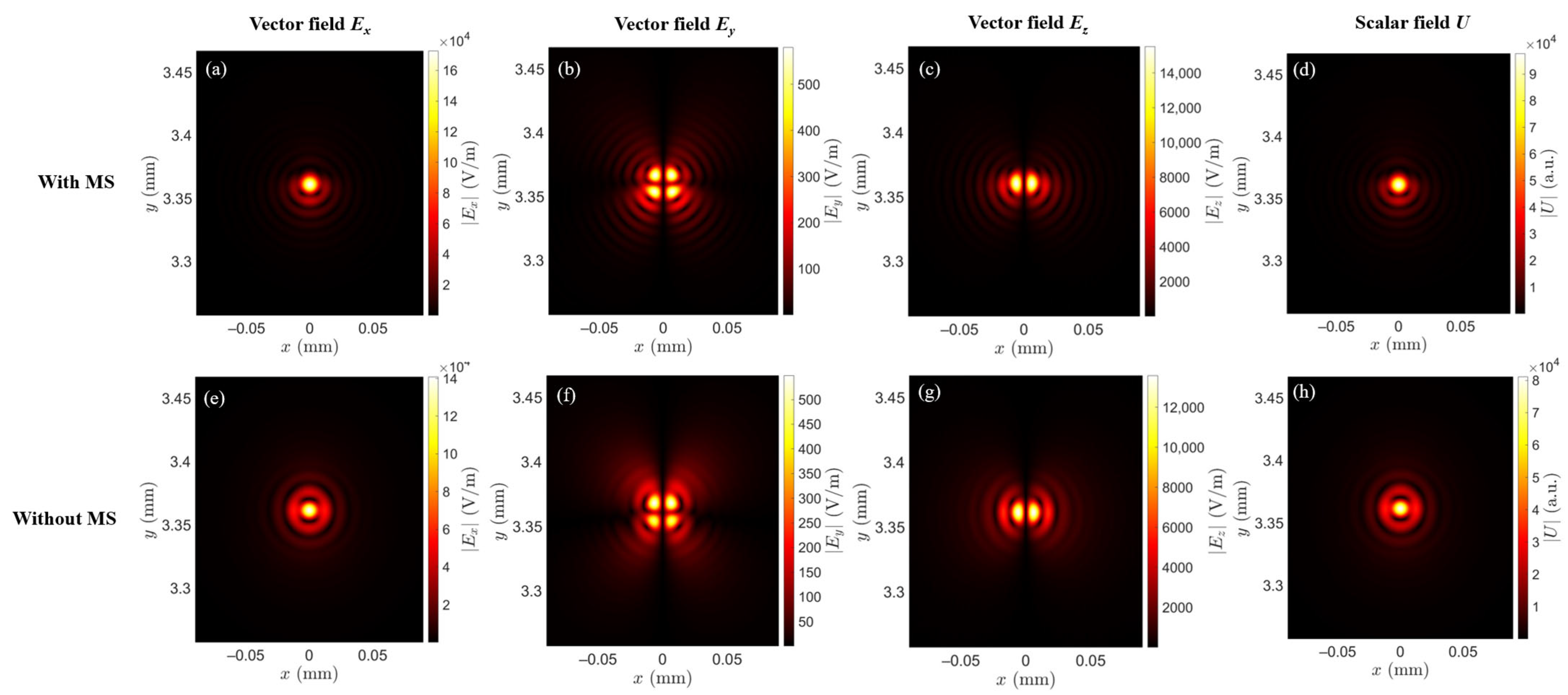
2.1. Properties of Vector Fields

We consider a model where input and output fields are defined on parallel planar surfaces, with optical component(s) sandwiched between them. The field is first prepared on an input plane, transmitted through optical component(s), and finally propagated to an output plane. This parallel planar configuration allows a more straightforward discussion as well as a simpler numerical implementation. A sequential connection of optical components is assumed such that an output field from one propagator becomes the input field of the next one. While it is possible to generalize this approach to non-parallel input and output planes using appropriate coordinate transformations, such extensions are beyond the scope of this work. Furthermore, for ease of data recording and computational efficiency, we assume that all fields are sampled on rectangular grids.

Before discussing the specifics of propagators, it is necessary to establish the vector field components to be addressed by them. We consider a monochromatic electromagnetic field with sign convention $\exp \left(-i\omega t\right)$, which comprises six components represented in Cartesian coordinates. With transverse electric field components E_x(x, y) and E_y(x, y) specified on a plane in a uniform media, the z-component electric field is dependent and can be calculated as [25]

$$E_z\left(x,y\right)=-{ℱ}^{-1}\left\{{\displaystyle \frac{k_xℱ\left\{E_x\right\}+k_yℱ\left\{E_y\right\}}{k_z}}\right\},$$

(1)

where $k_z=\sqrt{k^2-k_x^2-k_y^2}$, with k_x, k_y, and k_z being spatial wave numbers in the x-, y- and z-directions, respectively and k is wavenumber of the media; $ℱ\left\{\xi \right\}$ and ${ℱ}^{-1}\left\{\xi \right\}$ denote Fourier transform and its inverse, respectively. Moreover, we can evaluate the three magnetic field components on a plane as

$$H_l\left(x,y\right)={\displaystyle \frac{1}{k_0{Z}_0}}{ℱ}^{-1}\left\{k_mℱ\left\{E_n\right\}-k_nℱ\left\{E_m\right\}\right\},$$

(2)

where Z₀ is free space impedance, k₀ is free space wavenumber; l, m, and n are cyclic permutations of {x, y, z}. These relations between field components imply that only the transverse electric field components, E_x and E_y, need to be tracked as a wave propagates, and the other four components can be determined from Fourier transforms on demand. Consequently, the formulations for the propagators in the following sections will primarily focus on the evolution of E_x and E_y.

2.2. Propagation in Free Space

Firstly, we discuss vector field propagation in free space between optical components. In free space, all the field components are decoupled, and propagation can be done to each component separately using the ASM [25]. Considering input field components, $E_{x\left(y\right),\mathrm{in}}$, prepared on an input plane z = 0, we can determine output field components on an output plane z = d as

$$E_{x\left(y\right),\mathrm{out}}\left(x, y\right)={ℱ}^{-1}\left\{H\left(k_x, k_y\right)ℱ\left\{E_{x\left(y\right),\mathrm{in}}\left(x, y\right)\right\}\right\},$$

(3)

where

$$H\left(k_x,k_y\right)=\exp \left(i\sqrt{k^2-k_x^2-k_y^2}d\right)$$

(4)

is the transfer function for uniform space with k being wavenumber for the filling material between the two planes. While with its simple expression, various chirp z-transform techniques can be applied to shift the output window relative to the input window and to scale the window size up or down [24], which is particularly useful where beam size change drastically, such as propagating an off-axis, converging wavefront from the exit pupil of a system to its image plane. It should be noted that the GDM going to be described next can also be used for free-space propagation. However, the ASM is numerically more efficient and is widely employed in the MS-refractive hybrid system examples presented in this work.

2.3. Propagation Through Refractive Optics

Refractive elements are crucial in the design of MS-refractive hybrid lenses. Simulating beam propagation through such systems requires selecting a solver capable of handling curved elements. However, rigorous electromagnetic solvers like the finite-difference frequency-domain (FDFD) method become impractical for centimeter-scale lenses due to their computational complexity. This makes the use of a lightweight propagator essential. The RFM provides an approximate solution by decomposing an input scalar field (i.e., polarization effects are ignored) into pencil rays whose directions and magnitudes locally match with input wavefront; These rays are then traced through curved surfaces and information such as ray density, optical path length are used to estimate output scalar field. While it is possible to generalize RFM to account for polarization effects, its inherently simple formulation introduces several limitations: (1) it does not account for ray path diffraction, leading to inaccurate results near foci or caustics, and (2) it is not suitable to simulate complex wavefronts, such as vortex beams. These limitations will be illustrated in more detail later.

Consequently, a more general propagator for vector field propagation through refractive optics is required, and we introduce GDM to fill this gap. In GDM, an arbitrary field is initially broken down into Gaussian beams. These beams are subsequently propagated through an optical system in a locally paraxial manner along their central rays. The resulting field at any location, whether in the final plane or an intermediate one, is then reconstructed by coherently summing the complex field contributions from each Gaussian beam after its propagation. GDM has been implemented in commercial optical design software, such as FRED, though its numerical implementation has limited documentation. Recently, Ashcraft et al. provided a pedagogical overview of scalar field propagation through complex optical systems using GDM [26]. Building on their work, we developed our own GDM implementation with further consideration of the following factors: (1) explicit inclusion of beam polarization in the formulations, (2) adaptive Gaussian beam radii and curvatures on the input plane, and (3) allowance for non-zero Gaussian beam inclinations on the input plane. This results in a general propagator that, is given an input transverse electric field $E_{x\left(y\right),\mathrm{in}}$ on an input plane, can determine the corresponding output transverse electric field $E_{x\left(y\right),\mathrm{out}}$ after passing through refractive optics. In the following subsections, the steps of our GDM implementation are discussed.

2.3.1. Gaussian Beam Decomposition

The evolution of a Gaussian beam in a homogeneous media is most concisely expressed as

$$E\left(r,z\right)=E_0\exp \left(i{\displaystyle \frac{k}{2}}{r}^T{Q}^{-1}\left(z\right)r\right)\exp \left(ikz\right),$$

(5)

where E₀ is on-axis polarization, $Q^{-1}$ is a 2-by-2 complex beam parameter matrix that encodes information about wavefront curvatures and beam widths, z is the spatial coordinate along propagation direction, and $r={\left[x, y\right]}^T$ is the spatial coordinate on a z-plane transversal to propagation axis with origin centered at the propagation axis.

Given E_x(y),in on an input plane, the first step is decomposing $E_{x\left(y\right),\mathrm{in}}$ into gaussian beams described by Equation (5). Since the two field components are generally independent, decomposition must be performed separately. The process is similar for both components, so we use $U_{\mathrm{in}}$ to represent either component, noting specific considerations for each component where relevant. The objective is to determine a set of Gaussian beams whose superposition best approximates $U_{\mathrm{in}}$. Based on Equation (5), each Gaussian beam on the input plane is generally astigmatic and is defined by five parameters: (1) axis position, (2), direction, (3) wavefront curvatures, (4) beam widths, and (5) polarization. Due to the non-orthogonality of Gaussian beams, there is no unique solution for determining these parameters across all beams [26]. In the following, we outline our approach, starting with the selection of beam center positions.

Various sampling schemes for placing Gaussian beams have been proposed in the literature [26,27,28]. In this work, we adopt a Fibonacci spiral pattern for positioning Gaussian beams on the input plane, as this pattern has been shown to offer higher accuracy for input fields lacking clear symmetry [27]. Given N Gaussian beams to be arranged in a Fibonacci spiral pattern with radius R, Gaussian beam center positions in polar coordinates are given by

$$r_{\mathbf{i}}=R \sqrt{{\displaystyle \frac{i}{N}}},$$

(6a)

$${\theta }_i={\displaystyle \frac{4\pi }{1+\sqrt{5}}}i,$$

(6b)

where i = {1, 2…N} is the index of the Gaussian beams. In general, the origin of a pattern is shifted to the amplitude centroid of U_in, and the pattern radius R is estimated from the amplitude’s second moment width measured with respect to amplitude centroid. On the other hand, the number of Gaussian beams N depends largely on the complexity of the input field. In this work where we employ GBD to propagate complex and highly structured input fields, we typically set N = 10,000. For beams with simpler profiles, such as a super Gaussian beam with a flat wavefront, an accurate representation can be achieved using only a small number (N < 1000) of Gaussian beams in the decomposition process.

Refer to Figure 2a, a Gaussian beam starting on an input plane with position $r_{\mathrm{in}}$ has a propagation direction ${\widehat{k}}_{\mathrm{in}}$, which can be estimated from phase gradient as

$${\widehat{k}}_{\mathrm{in}}=k_{x,\mathrm{in}}\widehat{x}+k_{y,\mathrm{in}}\widehat{y}+k_{z,\mathrm{in}}\widehat{z}={\displaystyle \frac{1}{k_{\mathrm{in}}}}\left[{\displaystyle \frac{\partial {\varphi }_{\mathrm{in}}}{\partial x}}\widehat{x}+{\displaystyle \frac{\partial {\varphi }_{\mathrm{in}}}{\partial y}}\widehat{y}+\sqrt{k_{\mathrm{in}}^2-{\left({\displaystyle \frac{\partial {\varphi }_{\mathrm{in}}}{\partial x}}\right)}^2-{\left({\displaystyle \frac{\partial {\varphi }_{\mathrm{in}}}{\partial y}}\right)}^2}\widehat{z}\right],$$

(7)

with $k_{\mathrm{in}}$ being input region wavenumber and ${\varphi }_{\mathrm{in}}=\mathrm{Arg}\left[U_{\mathrm{in}}\right]$. Finite difference calculation can be applied to approximate the partial derivatives. To help discussion (Figure 2a), we will refer to planes transverse to ${\widehat{k}}_{\mathrm{in}}$ as input transverse planes ${\mathrm{P}}_{\mathrm{in}}$, with the one intersecting $r_{\mathrm{in}}$ denoted as the principal input transverse plane ${\mathrm{P}}_{\mathrm{in},0}$. Note that each Gaussian beam has a unique ${\mathrm{P}}_{\mathrm{in},0}$ but can have an infinite number of ${\mathrm{P}}_{\mathrm{in}}$.

An input field may exhibit a converging or diverging wavefront with non-zero phase curvature. To achieve the best fit while minimizing the number of Gaussian beams used in a decomposition step, Gaussian wavefront curvatures can be incorporated by approximating the local wavefront near each Gaussian beam with a quadratic function defined by its principal curvatures (Figure 2b). Principal curvatures represent the maximum and minimum curvature values at a point, with the directions in which these extrema occur known as the principal directions. To obtain principal curvatures and principal directions for a Gaussian beam on the input plane, we first construct the shape operator matrix [29]:

$$S={\displaystyle \frac{1}{\sqrt{1+z_x^2+z_y^2}}}{\left[\begin{array}{cc}1+z_x^2& z_x{z}_y\\ z_x{z}_y& 1+z_y^2\end{array}\right]}^{-1}\left[\begin{array}{cc}{z}_{xx}& z_{xy}\\ z_{xy}& z_{yy}\end{array}\right],$$

(8)

where $z=-{\displaystyle \frac{\mathrm{Arg}\left[U_{\mathrm{in}}\right]}{k_{z,\mathrm{in}}}}$ and the subscripts denote partial derivatives (e.g., $z_{xx}={\displaystyle \frac{{\partial }^{2}z}{\partial x^2}}$). This matrix is constructed using the following basis on the principal input transverse plane:

$$u=\widehat{x}+z_x\widehat{z},$$

(9a)

$$v=\widehat{y}+z_y\widehat{z}.$$

(9b)

Principal curvatures and principal directions are obtained from solving the eigen-problem:

$$S=O{C}_{\left(s,p\right)}{O}^{-1},$$

(10)

where

$$C_{\left(s,p\right)}=\left[\begin{array}{cc}{C}_s& 0\\ 0& C_p\end{array}\right],$$

(11)

and

$$O=\left[\begin{array}{cc}{s}_{uv}& p_{uv}\end{array}\right]=\left[\begin{array}{cc}{s}_u& p_u\\ s_v& p_v\end{array}\right],$$

(12)

with C_s and C_p are principal curvatures; $s_{uv}$ and $p_{uv}$ are the associated principal directions in the (u, v) basis. The principal directions serve as a convenient basis to express a Gaussian beam in input region, as they are orthogonal and lie on ${\mathrm{P}}_{\mathrm{in},0}$. In the global coordinate system, they are expressed as

$${\widehat{s}}_{\mathrm{in}}={\displaystyle \frac{s_{u}u+s_{v}v}{\left|s_{u}u+s_{v}v\right|}},$$

(13a)

$${\widehat{p}}_{\mathrm{in}}={\displaystyle \frac{p_{u}u+p_{v}v}{\left|p_{u}u+p_{v}v\right|}}.$$

(13b)

Note (${\widehat{s}}_{\mathrm{in}}, {\widehat{p}}_{\mathrm{in}}, {\widehat{k}}_{\mathrm{in}}$) form an orthonormal basis for a Gaussian beam in the input region.

Principal curvatures give the local wavefront curvature and are part of the information required to construct the complex beam parameter matrix $Q^{-1}$ in Equation (5). What remains to be determined is beam width. This is achieved by computing the covariance matrix of input field amplitude centered at each Gaussian beam on the input plane:

$${\Sigma }_{\left(x,y\right)}=\left[\begin{array}{cc}{\mathsf{\Sigma }}_{xx}& {\mathsf{\Sigma }}_{yx}\\ {\mathsf{\Sigma }}_{xy}& {\mathsf{\Sigma }}_{yy}\end{array}\right],$$

(14)

where

$${\mathsf{\Sigma }}_{xx}={{\displaystyle \iint }}_{\mathsf{\Lambda }}{\overline{U}}_{\mathrm{in}}\left(\overline{x},\overline{y}\right){\overline{x}}^{2}dxdy,$$

(15a)

$${\mathsf{\Sigma }}_{yy}={{\displaystyle \iint }}_{\mathsf{\Lambda }}{\overline{U}}_{\mathrm{in}}\left(\overline{x},\overline{y}\right){\overline{y}}^{2}dxdy,$$

(15b)

$${\mathsf{\Sigma }}_{xy}={\mathsf{\Sigma }}_{yx}={{\displaystyle \iint }}_{\mathsf{\Lambda }}{\overline{U}}_{\mathrm{in}}\left(\overline{x},\overline{y}\right)\overline{x}\overline{y}dxdy.$$

(15c)

Λ is a covariance bound to limit beam width and ${\overline{U}}_{\mathrm{in}}$ is the magnitude of $U_{\mathrm{in}}$ normalized to unity in Λ; $\overline{x}$ and $\overline{y}$ are relative positions on the input plane centered at the Gaussian beam center. Referring to Figure 2c, ${\Sigma }_{\left(x,y\right)}$ represents amplitude distribution calculated on the input plane and is expressed in the $\left(\widehat{x}, \widehat{y}\right)$ basis, while what we need is a distribution on ${\mathrm{P}}_{\mathrm{in},0}$ and expressed in the (${\widehat{s}}_{\mathrm{in}}, {\widehat{p}}_{\mathrm{in}}$) basis. Approximation based on geometrical projection is made by first finding the principal axes, $e_1$ and $e_2$, of the ellipse associated with ${\Sigma }_{\left(x,y\right)}$, and projecting them onto ${\mathrm{P}}_{\mathrm{in},0}$:

$$e_1^{\prime }=e_1-\left(e_1\cdot {\widehat{k}}_{\mathrm{in}}\right){\widehat{k}}_{\mathrm{in}},$$

(16a)

$$e_2^{\prime }=e_2-\left(e_2\cdot {\widehat{k}}_{\mathrm{in}}\right){\widehat{k}}_{\mathrm{in}}.$$

(16b)

Here, $e_1^{\prime }$ and $e_2^{\prime }$ are a set of conjugated axes for an ellipse on ${\mathrm{P}}_{\mathrm{in},0}$. The corresponding principal axes of the ellipse are obtained from superposition of $e_1^{\prime }$ and $e_2^{\prime }$ [30]:

$$p_1=e_1^{\prime }\cos (t_0)+e_2^{\prime }\sin (t_0),$$

(17a)

$$p_2=e_1^{\prime }\cos (t_0+\pi /2)+e_2^{\prime }\sin (t_0+\pi /2),$$

(17b)

with

$$t_0={\displaystyle \frac{1}{2}}{\cot }^{-1}\left({\displaystyle \frac{e_1^{\prime }\cdot e_1^{\prime }-e_2^{\prime }\cdot e_2^{\prime }}{2e_1^{\prime }\cdot e_2^{\prime }}}\right).$$

(18)

The principal axes $p_1$ and $p_2$ are on the ${\mathrm{P}}_{\mathrm{in},0}$ as well. The covariance matrix in the (${\widehat{s}}_{\mathrm{in}}, {\widehat{p}}_{\mathrm{in}}$) basis is then obtained with a proper change of basis:

$${\Sigma }_{\left(s,p\right)}=O_{\left(s,p\right)\leftarrow \left(p_1,p_2\right)}{\Sigma }_{\left(p_1,p_2\right)}{O}_{\left(p_1,p_2\right)\leftarrow \left(s,p\right)},$$

(19)

where

$${\Sigma }_{\left(p_1,p_2\right)}=\left[\begin{array}{cc}\left|p_1\right|& 0\\ 0& \left|p_2\right|\end{array}\right],$$

(20)

$$O_{\left(s,p\right)\leftarrow \left(p_1,p_2\right)}=O_{\left(p_1,p_2\right)\leftarrow \left(s,p\right)}^{-1}=\left[\begin{array}{cc}{\widehat{s}}_{\mathrm{in}}\cdot {\widehat{p}}_1& {\widehat{s}}_{\mathrm{in}}\cdot {\widehat{p}}_2\\ {\widehat{p}}_{\mathrm{in}}\cdot {\widehat{p}}_1& {\widehat{p}}_{\mathrm{in}}\cdot {\widehat{p}}_2\end{array}\right].$$

(21)

An estimation of the complex beam parameter matrix of a Gaussian beam on ${\mathrm{P}}_{\mathrm{in},0}$ can be made as

$$Q_{\mathrm{in},0}^{-1}=-C_{\left(s,p\right)}+{\displaystyle \frac{i}{k_{\mathrm{in}}}}{\Sigma }_{\left(s,p\right)}^{-1},$$

(22)

The next step is to calculate the amplitude coefficients of individual Gaussian beams. Referring to Figure 2a, the normalized amplitudes contributed by a Gaussian beam (with index j) to sampling points $r_i$, i = {1, 2…M}, on the input plane are

$$g_j\left(r_i\right)={\displaystyle \frac{1}{\sqrt{\det \left|A_{\mathrm{in}}+B_{\mathrm{in}}{Q}_{\mathrm{in},0}^{-1}\right|}}}\exp \left(i{k}_{\mathrm{in}}\left({\displaystyle \frac{1}{2}}{\overline{r}}_i^T{Q}_{\mathrm{in}}^{-1}{\overline{r}}_i+{\mathsf{\Delta }}_{\mathrm{in}}\right)\right),$$

(23)

where

$${\overline{r}}_i=\left[\begin{array}{c}\left(r_i-r_{\mathrm{in}}\right)\cdot {\widehat{s}}_{\mathrm{in}}\\ \left(r_i-r_{\mathrm{in}}\right)\cdot {\widehat{p}}_{\mathrm{in}}\end{array}\right]$$

(24)

is relative position of $r_i$ with respect to $r_{\mathrm{in}}$ in the (${\widehat{s}}_{\mathrm{in}}, {\widehat{p}}_{\mathrm{in}}$) basis, and

$$Q_{\mathrm{in}}^{-1}=\left(C_{\mathrm{in}}+D_{\mathrm{in}}{Q}_{\mathrm{in},0}^{-1}\right){\left(A_{\mathrm{in}}+B_{\mathrm{in}}{Q}_{\mathrm{in},0}^{-1}\right)}^{-1}$$

(25)

is the complex beam parameter matrix on the ${\mathrm{P}}_{\mathrm{in}}$ that intersects $r_i$, with

$$M_{\mathrm{in}}=\left[\begin{array}{cc}{A}_{\mathrm{in}}& B_{\mathrm{in}}\\ C_{\mathrm{in}}& D_{\mathrm{in}}\end{array}\right]=\left[\begin{array}{cc}I& {\mathsf{\Delta }}_{\mathrm{in}}I\\ 0& I\end{array}\right],$$

(26)

is transfer matrix for free space in the input region over a signed distance ${\mathsf{\Delta }}_{\mathrm{in}}=\left(r_i-r_{\mathrm{in}}\right)\cdot {\widehat{k}}_{\mathrm{in}}$; 0 and I are 2-by-2 zero matrix and identity matrix, respectively. Ideally, for a set of N Gaussian beams and M sampling points with known input field amplitudes, the amplitude coefficient of individual Gaussian beam $c_j$, j = {1, 2…N}, is determined such that the following matrix equation is satisfied:

$$\underset{G}{\underbrace{\left[\begin{array}{ccc}{g}_1\left(r_1\right)& \cdots & g_N\left(r_1\right)\\ ⋮& \ddots & ⋮\\ g_1\left(r_M\right)& \cdots & g_N\left(r_M\right)\end{array}\right]}}\underset{c}{\underbrace{\left[\begin{array}{c}{c}_1\\ ⋮\\ c_N\end{array}\right]}}\triangleq \underset{U}{\underbrace{\left[\begin{array}{c}{U}_{\mathrm{in}}\left(r_1\right)\\ ⋮\\ U_{\mathrm{in}}\left(r_M\right)\end{array}\right]}},$$

(27)

Generally, $M\gg N$ so the pseudo-inverse of G could be applied to obtain the amplitude coefficients as

$$\mathbf{c}={\left({\mathbf{G}}^{†}\mathbf{G}\right)}^{-1}{\mathbf{G}}^{†}\mathbf{U},$$

(28)

where the daggers denote Hermitian conjugates. In practice, Gaussian beams are highly compact such that the matrix G is constructed as a sparse matrix and is solved efficiently as a least squared problem in MATLAB (R2024a) as c = lsqminnorm(G, U). The accuracy of this step can be estimated as

$$\mathrm{RMS} \mathrm{error}:={\displaystyle \frac{{\sum }_i\left[{\overline{U}}_{\mathrm{in}}\left(r_i\right)-U_{\mathrm{in}}\left(r_i\right)\right]{\left[{\overline{U}}_{\mathrm{in}}\left(r_i\right)-U_{\mathrm{in}}\left(r_i\right)\right]}^{*}}{{\sum }_i{U}_{\mathrm{in}}\left(r_i\right)U_{\mathrm{in}}{\left(r_i\right)}^{*}}},$$

(29)

where the asterisks denote complex conjugates, and ${\overline{U}}_{\mathrm{in}}\left(r_i\right)=\sum _j{c}_j{g}_j\left(r_i\right)$ is input field reconstructed from Gaussian beam superposition. A small error can be attained with an increased number of Gaussian beams used in a decomposition process. For all experiments in this work, we treat an RMS error below 0.01% as an accepted accuracy standard. Finally, for a Gaussian beam with amplitude coefficient c, the associated polarization is estimated from the orthogonality condition $E_{\mathrm{in}}\cdot {\widehat{k}}_{\mathrm{in}}=0$ as

$${\mathbf{E}}_{\mathrm{in}}=\{\begin{array}{ll}c\hat{\mathbf{x}}-\frac{k_{x,\mathrm{in}}c}{k_{z,\mathrm{in}}}\hat{\mathbf{z}}& \mathrm{for} U_{\mathrm{in}}≔E_{x,\mathrm{in}}\\ c\hat{\mathbf{y}}-\frac{k_{y,\mathrm{in}}c}{k_{z,\mathrm{in}}}\hat{\mathbf{z}}& \mathrm{for} U_{\mathrm{in}}≔E_{y,\mathrm{in}}\end{array}.$$

(30)

To conclude, for a transversal field component $E_{x\left(y\right),\mathrm{in}}$, a set of Gaussian beams is prepared on the input plane with positions arranged as a Fibonacci spiral pattern and beam directions calculated from wavefront normal (Equation (7)); Local wavefront curvatures and amplitude variations are used to construct the complex beam parameter matrix of the individual beam (Equation (22)), and a least square fit is applied to determine beam polarizations (Equation (30)).

2.3.2. Gaussian Beam Propagation

Once an input field component is decomposed into a set of Gaussian beams, each beam is propagated through the refractive optics to the output plane. Given the highly localized nature of Gaussian beams around their waists, field contributions become negligible at distances far from these waists. This locality allows the GDM to effectively simulate propagation through non-paraxial refractive optics. Two main aspects of Gaussian beam propagation are addressed in this section: (1) beam profile evolution, modeled with a 4-by-4 differential transfer matrix [26], and (2) polarization evolution, involving polarization ray tracing technique [31]. Details for these calculations are provided in this section.

Gaussian beam tracing is a well-established approach that formulates a 4-by-4 differential transfer matrix and evaluates the evolution of complex beam parameter along an individual Gaussian beam path. The finite difference technique is used to construct the transfer matrix. Referring to Figure 3, a base ray aligned with an individual Gaussian beam on the input plane is defined, along with four parabasal rays positioned around it. Among them, two are shifted from the base ray:

$$r_{\mathrm{in}}^{\left(s,\mathsf{\Delta }h\right)}=r_{\mathrm{in}}+\mathsf{\Delta }h{\widehat{s}}_{\mathrm{in}},$$

(31a)

$$r_{\mathrm{in}}^{\left(p,\mathsf{\Delta }h\right)}=r_{\mathrm{in}}+\mathsf{\Delta }h{\widehat{p}}_{\mathrm{in}},$$

(31b)

and the other two are tilted with respect to the base ray:

$${\widehat{k}}_{\mathrm{in}}^{\left(s,\mathsf{\Delta }k\right)}={\displaystyle \frac{{\widehat{k}}_{\mathrm{in}}+\mathsf{\Delta }k{\widehat{s}}_{\mathrm{in}}}{\left|{\widehat{k}}_{\mathrm{in}}+\mathsf{\Delta }k{\widehat{s}}_{\mathrm{in}}\right|}},$$

(32a)

$${\widehat{k}}_{\mathrm{in}}^{\left(p,\mathsf{\Delta }k\right)}={\displaystyle \frac{{\widehat{k}}_{\mathrm{in}}+\mathsf{\Delta }k{\widehat{p}}_{\mathrm{in}}}{\left|{\widehat{k}}_{\mathrm{in}}+\mathsf{\Delta }k{\widehat{p}}_{\mathrm{in}}\right|}}.$$

(32b)

In Equations (31) and (32), the first character in the superscripts indicates the transverse direction (${\widehat{s}}_{\mathrm{in}}$ or ${\widehat{p}}_{\mathrm{in}}$), while the second character specifies whether it represents a shift ($\mathsf{\Delta }h$) or a tilt ($\mathsf{\Delta }k$). This notation will be used hereafter. Parabasal rays are launched to estimate the differential ray data of a base ray, requiring a small shift or tilt. In this work, we set $\mathsf{\Delta }h={10}^{-9} \mathrm{m}$ and $\mathsf{\Delta }k={10}^{-9}$.

The base ray is initiated on the input plane and traced through the refractive optics to the output plane. As illustrated in Figure 3, this base ray reaches a position $r_{\mathrm{out}}$ with direction ${\widehat{k}}_{\mathrm{out}}$ on the output plane. In the output region, similar to the input region, planes transverse to ${\widehat{k}}_{\mathrm{out}}$ are referred to as the output transverse planes ${\mathrm{P}}_{\mathrm{out}}$, with the one intersecting $r_{\mathrm{out}}$ designated as the principal output transverse plane ${\mathrm{P}}_{\mathrm{out},0}$. Meanwhile, the four paraxial rays are initiated on ${\mathrm{P}}_{\mathrm{in},0}$, traced to ${\mathrm{P}}_{\mathrm{out},0}$, and denoted following the aforementioned notations. For example, $r_{\mathrm{out}}^{\left(p,\mathsf{\Delta }h\right)}$ represents the position on ${\mathrm{P}}_{\mathrm{out},0}$ for the parabasal ray shifted in the ${\widehat{p}}_{\mathrm{in}}$ direction.

The objective is to find the transfer matrix $M_c$ relating complex beam parameters across ${\mathrm{P}}_{\mathrm{in},0}$ to ${\mathrm{P}}_{\mathrm{out},0}$. This is achieved by first defining an orthogonal basis on ${\mathrm{P}}_{\mathrm{out},0}$:

$${\widehat{s}}_{\mathrm{out}}={\widehat{k}}_{\mathrm{out}}\times \widehat{z},$$

(33a)

$${\widehat{p}}_{\mathrm{out}}={\widehat{k}}_{\mathrm{out}}\times {\widehat{s}}_{\mathrm{out}}.$$

(33b)

(${\widehat{s}}_{\mathrm{out}}, {\widehat{p}}_{\mathrm{out}}, {\widehat{k}}_{\mathrm{out}}$) is an orthonormal basis for a Gaussian beam in the output region. Note it is assumed that the output plane has a surface normal in the z-direction, which conforms to our model as described in Section 2.1. To obtain $M_c$, it is convenient to express a base ray on ${\mathrm{P}}_{\mathrm{out},0}$ using the (${\widehat{s}}_{\mathrm{out}}, {\widehat{p}}_{\mathrm{out}}, {\widehat{k}}_{\mathrm{out}}$) basis:

$${\tilde{r}}_{\mathrm{out}}=O_{\left(s_{\mathrm{out}},p_{\mathrm{out}},k_{\mathrm{out}}\right)\leftarrow \left(x,y,z\right)}{r}_{\mathrm{out}}=\left[\begin{array}{c}{\tilde{x}}_{\mathrm{out}}\\ {\tilde{y}}_{\mathrm{out}}\\ {\tilde{z}}_{\mathrm{out}}\end{array}\right],$$

(34a)

$${\tilde{\widehat{k}}}_{\mathrm{out}}=O_{\left(s_{\mathrm{out}},p_{\mathrm{out}},k_{\mathrm{out}}\right)\leftarrow \left(x,y,z\right)}{\widehat{k}}_{\mathrm{out}}=\left[\begin{array}{c}{\tilde{l}}_{\mathrm{out}}\\ {\tilde{m}}_{\mathrm{out}}\\ {\tilde{n}}_{\mathrm{out}}\end{array}\right],$$

(34b)

where

$$O_{\left(s_{\mathrm{out}},p_{\mathrm{out}},k_{\mathrm{out}}\right)\leftarrow \left(x,y,z\right)}=\left[\begin{array}{c}\begin{array}{c}{\widehat{s}}_{\mathrm{out}}^T\\ {\widehat{p}}_{\mathrm{out}}^T\end{array}\\ {\widehat{k}}_{\mathrm{out}}^T\end{array}\right].$$

(35)

is a unitary matrix for basis transformation. Similar operations are applied to the parabasal rays. For example, ${\tilde{r}}_{\mathrm{out}}^{\left(p,\mathsf{\Delta }h\right)}=O_{\left(s_{\mathrm{out}},p_{\mathrm{out}},k_{\mathrm{out}}\right)\leftarrow \left(x,y,z\right)}{r}_{\mathrm{out}}^{\left(p,\mathsf{\Delta }h\right)}={\left[\begin{array}{ccc}{\tilde{x}}_{\mathrm{out}}^{\left(p,\mathsf{\Delta }h\right)}& {\tilde{y}}_{\mathrm{out}}^{\left(p,\mathsf{\Delta }h\right)}& {\tilde{z}}_{\mathrm{out}}^{\left(p,\mathsf{\Delta }h\right)}\end{array}\right]}^T$. With all rays transferred to the (${\widehat{s}}_{\mathrm{out}}, {\widehat{p}}_{\mathrm{out}}, {\widehat{k}}_{\mathrm{out}}$) basis, the finite difference technique can be applied to obtain the transfer matrix $M_c$:

$$M_c=\left[\begin{array}{cc}{A}_c& B_c\\ C_c& D_c\end{array}\right]=\left[\begin{array}{cc}\underset{A_c}{\underbrace{\left[\begin{array}{cc}{\displaystyle \frac{{\tilde{x}}_{\mathrm{out}}^{\left(s,\mathsf{\Delta }h\right)}-{\tilde{x}}_{\mathrm{out}}}{\mathsf{\Delta }h}}& {\displaystyle \frac{{\tilde{x}}_{\mathrm{out}}^{\left(p,\mathsf{\Delta }h\right)}-{\tilde{x}}_{\mathrm{out}}}{\mathsf{\Delta }h}}\\ {\displaystyle \frac{{\tilde{y}}_{\mathrm{out}}^{\left(s,\mathsf{\Delta }h\right)}-{\tilde{y}}_{\mathrm{out}}}{\mathsf{\Delta }h}}& {\displaystyle \frac{{\tilde{y}}_{\mathrm{out}}^{\left(s,\mathsf{\Delta }h\right)}-{\tilde{y}}_{\mathrm{out}}}{\mathsf{\Delta }h}}\end{array}\right]}}& \underset{B_c}{\underbrace{\left[\begin{array}{cc}{\displaystyle \frac{{\tilde{x}}_{\mathrm{out}}^{\left(s,\mathsf{\Delta }k\right)}-{\tilde{x}}_{\mathrm{out}}}{\mathsf{\Delta }k}}& {\displaystyle \frac{{\tilde{x}}_{\mathrm{out}}^{\left(p,\mathsf{\Delta }k\right)}-{\tilde{x}}_{\mathrm{out}}}{\mathsf{\Delta }k}}\\ {\displaystyle \frac{{\tilde{y}}_{\mathrm{out}}^{\left(s,\mathsf{\Delta }k\right)}-{\tilde{y}}_{\mathrm{out}}}{\mathsf{\Delta }k}}& {\displaystyle \frac{{\tilde{y}}_{\mathrm{out}}^{\left(p,\mathsf{\Delta }k\right)}-{\tilde{y}}_{\mathrm{out}}}{\mathsf{\Delta }k}}\end{array}\right]}}\\ \underset{C_c}{\underbrace{\left[\begin{array}{cc}{\displaystyle \frac{{\tilde{l}}_{\mathrm{out}}^{\left(s,\mathsf{\Delta }h\right)}-{\tilde{l}}_{\mathrm{out}}}{\mathsf{\Delta }h}}& {\displaystyle \frac{{\tilde{l}}_{\mathrm{out}}^{\left(p,\mathsf{\Delta }h\right)}-{\tilde{l}}_{\mathrm{out}}}{\mathsf{\Delta }h}}\\ {\displaystyle \frac{{\tilde{m}}_{\mathrm{out}}^{\left(s,\mathsf{\Delta }h\right)}-{\tilde{m}}_{\mathrm{out}}}{\mathsf{\Delta }h}}& {\displaystyle \frac{{\tilde{m}}_{\mathrm{out}}^{\left(p,\mathsf{\Delta }h\right)}-{\tilde{m}}_{\mathrm{out}}}{\mathsf{\Delta }h}}\end{array}\right]}}& \underset{D_c}{\underbrace{\left[\begin{array}{cc}{\displaystyle \frac{{\tilde{l}}_{\mathrm{out}}^{\left(s,\mathsf{\Delta }k\right)}-{\tilde{l}}_{\mathrm{out}}}{\mathsf{\Delta }k}}& {\displaystyle \frac{{\tilde{l}}_{\mathrm{out}}^{\left(p,\mathsf{\Delta }k\right)}-{\tilde{l}}_{\mathrm{out}}}{\mathsf{\Delta }k}}\\ {\displaystyle \frac{{\tilde{m}}_{\mathrm{out}}^{\left(s,\mathsf{\Delta }k\right)}-{\tilde{m}}_{\mathrm{out}}}{\mathsf{\Delta }k}}& {\displaystyle \frac{{\tilde{m}}_{\mathrm{out}}^{\left(s,\mathsf{\Delta }k\right)}-{\tilde{m}}_{\mathrm{out}}}{\mathsf{\Delta }k}}\end{array}\right]}}\end{array}\right].$$

(36)

The complex beam parameter matrix on ${\mathrm{P}}_{\mathrm{out},0}$ is calculated through its matrix elements as

$$Q_{\mathrm{out},0}^{-1}=\left(C_c+D_c{Q}_{\mathrm{in},0}^{-1}\right){\left(A_c+B_c{Q}_{\mathrm{in},0}^{-1}\right)}^{-1},$$

(37)

and will be used in the next subsection for Gaussian beam superposition.

In this work, a clipping rule is employed during raytracing when a hard aperture is encountered: a Gaussian beam is entirely blocked if any associated ray, whether the base ray or parabasal rays, is obstructed. While more advanced methods to model edge effects on Gaussian beams are reported [32], they are beyond the scope of this study.

Equation (37) describes the evolution of the beam profile as a Gaussian beam propagates from the input region to the output region, but it does not account for polarization changes across interfaces in between. To track polarization throughout the propagation, we adopt the concept of polarization ray tracing [31]. In this approach, the polarization of a base ray is updated as it is traced through each surface. Given that the associated Gaussian beam is sufficiently compact, its local polarization can be considered homogeneous and effectively represented by the base ray’s polarization.

Considering an incident ray with direction ${\widehat{k}}_i$ and polarization $E_i$ has an intercept with a refractive surface with surface normal at the intercept is $\widehat{n}$. The refracted ray has a direction ${\widehat{k}}_o$ determined from the Snell’s law, and the objective is to find an expression of refracted ray polarization $E_o$ in the global coordinate system. Still, it is convenient to first define surface-ray interactions in a surface’s local coordinate systems:

$${\widehat{s}}_i={\widehat{s}}_o={\widehat{k}}_i\times \widehat{n},$$

(38a)

$${\widehat{p}}_i={\widehat{k}}_i\times {\widehat{s}}_i,$$

(38b)

$${\widehat{p}}_o={\widehat{k}}_o\times {\widehat{s}}_o.$$

(38c)

(${\widehat{s}}_i, {\widehat{p}}_i, {\widehat{k}}_i$) represents an orthonormal basis for the incident ray, and (${\widehat{s}}_o, {\widehat{p}}_o, {\widehat{k}}_o$) represents an orthonormal basis for the refracted ray. Using these two bases allows for efficient calculation of transmission coefficients across the interface in its local coordinates, while the overall polarization of the refracted ray is expressed in the global coordinate system. The impact of an interface on the ray polarization state is described by a 3-by-3 polarization raytracing matrix, P:

$$E_o=P{E}_i,$$

(39)

where

$$P=O_{o}T{O}_i^{-1}.$$

(40)

$O_i^{-1}$ is a matrix to transfer from the global coordinate system to the input side local coordinate system:

$$O_i^{-1}=\left[\begin{array}{c}{\widehat{s}}_i^T\\ {\widehat{p}}_i^T\\ {\widehat{k}}_i^T\end{array}\right],$$

(41)

$O_o$ is a matrix to transfer from the output side local coordinate system to the global coordinate system:

$$O_{\mathrm{out}}=\left[\begin{array}{ccc}{\widehat{s}}_o& {\widehat{p}}_o& {\widehat{k}}_o\end{array}\right],$$

(42)

and $T$ is a matrix with transmission coefficients as matrix elements; For a refractive surface, it is

$$\mathbf{T}=\left[\begin{array}{ccc}{t}_s& 0& 0\\ 0& t_p& 0\\ 0& 0& 1\end{array}\right]$$

(43)

with $t_s$ and $t_p$ being transmission coefficients for s- and p-polarizations, respectively. For an uncoated surface, these coefficients are described by the Fresnel equations; For a coated one, thin-film transmission coefficients should be used instead. Standard methods such as the transfer matrix method (TMM) [33] can be applied to obtain these coefficients. Incorporating these coefficients into polarization ray tracing requires careful attention to phase correction. Additionally, an ideal anti-reflection coating can be modeled by selecting appropriate values for these coefficients, as detailed in Section S1 of the Supplementary Information.

For a ray traced through N surfaces, we can concatenate the polarization raytracing matrix at each surface such that

$$\mathbf{P}={\mathbf{P}}_N\cdots {\mathbf{P}}_2{\mathbf{P}}_1$$

(44)

with P_i being the polarization raytracing matrix for the i-th surface. For each Gaussian beam, a polarization matrix as in Equation (41) is constructed to relate polarization on the input plane $E_{\mathrm{in}}$ (Equation (30)) to polarization on the output plane $E_{\mathrm{out}}=P{E}_{\mathrm{in}}$. Note that the phase accumulated from optical path length, being polarization-independent, is not considered in Equation (44).

In conclusion, each Gaussian beam in the input region is represented by a base ray and four parabasal rays, which are traced to the output region to capture the evolution of the individual beam profiles. The base ray also characterizes polarization variations resulting from refractions at interfaces.

2.3.3. Gaussian Beam Superposition

Referring to Figure 4, once Gaussian beam parameters in the output region are obtained from raytracing, the output field at any query point $r_o$ on the output plane can be computed through a superposition of the Gaussian beams. However, recall that Equation (37) defines the complex beam parameter matrix for a Gaussian beam on ${\mathrm{P}}_{\mathrm{out},0}$. To evaluate the field profile at $r_o$, a translation is needed from P_out,0 to P_out, which intersects with r_o. The corresponding transfer matrix is

$$M_{\mathrm{out}}=\left[\begin{array}{cc}{A}_{\mathrm{out}}& B_{\mathrm{out}}\\ C_{\mathrm{out}}& D_{\mathrm{out}}\end{array}\right]=\left[\begin{array}{cc}I& {\mathsf{\Delta }}_{\mathrm{out}}I\\ \mathbf{0}& I\end{array}\right],$$

(45)

where ${\mathsf{\Delta }}_{\mathrm{out}}=\left(r_o-r_{\mathrm{out}}\right)\cdot {\widehat{k}}_{\mathrm{out}}$, and the complex beam parameter matrix on ${\mathrm{P}}_{\mathrm{out}}$ is

$$Q_{\mathrm{out}}^{-1}=\left(C_{\mathrm{out}}+D_{\mathrm{out}}{Q}_{\mathrm{out},0}^{-1}\right){\left(A_{\mathrm{out}}+B_{\mathrm{out}}{Q}_{\mathrm{in},0}^{-1}\right)}^{-1}.$$

(46)

Finally, the output field contributed from an individual Gaussian beam at $r_o$ is

$$E\left(r_o\right)={\displaystyle \frac{E_{\mathrm{out}}}{\sqrt{\det \left|A_{\mathrm{out}}+B_{\mathrm{out}}{Q}_{\mathrm{out},0}^{-1}\right|}}}\exp \left(i\left({\displaystyle \frac{k_{\mathrm{out}}}{2}}{\overline{r}}_o^T{Q}_{\mathrm{out}}^{-1}{\overline{r}}_o+k_{\mathrm{out}}{\mathsf{\Delta }}_{\mathrm{out}}+k_0\mathrm{OPL} \right)\right),$$

(47)

with $k_{\mathrm{out}}$ being output region wavenumber, OPL being the optical path length of the base ray from ${\mathrm{P}}_{\mathrm{in},0}$ to ${\mathrm{P}}_{\mathrm{out},0}$, and

$${\overline{r}}_o=\left[\begin{array}{c}\left(r_o-r_{\mathrm{out}}\right)\cdot {\widehat{s}}_{\mathrm{out}}\\ \left(r_o-r_{\mathrm{out}}\right)\cdot {\widehat{p}}_{\mathrm{out}}\end{array}\right]$$

(48)

being the relative position of $r_o$ with respect to rout in the (${\widehat{s}}_{\mathrm{out}}, {\widehat{p}}_{\mathrm{out}}$) basis. The overall output field is obtained by summing the contributions from two sets of Gaussian beams: one representing $E_{x,\mathrm{in}}$ and the other representing $E_{y,\mathrm{in}}$. Following the discussion in Section 2.1, only the transverse components of the output field, $E_{x,\mathrm{out}}$ and $E_{y,\mathrm{out}}$, are recorded for further analysis or propagation. It is worth noting that the GDM formalism can be equally applied to reflective optics, although this work focuses exclusively on refractive optics. A simplified flowchart for key steps in GDM is shown in Figure 5.

Brief discussions on the numerical implementation of GDM are appropriate here. Although the formalism is expressed for individual Gaussian beams in prior sections, most vector-matrix and matrix-matrix operations can be efficiently broadcast across all beams, and GPU acceleration supports this process. Notably, we separate Gaussian beam propagation into two parts: one from ${\mathrm{P}}_{\mathrm{in},0}$ to ${\mathrm{P}}_{\mathrm{out},0}$ and the other from ${\mathrm{P}}_{\mathrm{out},0}$ to ${\mathrm{P}}_{\mathrm{out}}$ intersecting a query point $r_o$ (see Figure 4). This division could, in theory, be combined, allowing for simplification where calculation of the complex beam parameter matrix on ${\mathrm{P}}_{\mathrm{out},0}$ (Equation (37)) is bypassed, and the corresponding transfer matrices in Equations (36) and (45) are condensed into a single matrix $M=M_{\mathrm{out}}{M}_c$. Note that each Gaussian beam has a single pair of ${\mathrm{P}}_{\mathrm{in},0}$ and ${\mathrm{P}}_{\mathrm{out},0}$, resulting in one $M_c$. However, since $M_{\mathrm{out}}$ varies with $r_o$, data management proportional to the number of query points is required throughout propagation to directly compute $M$ for all combinations of Gaussian beams and query points, which can be computationally demanding when a large output window with fine resolution is involved. Our implementation limits array broadcasts across all query points to only when absolutely necessary.

To accelerate the Gaussian beam superposition process, interpolation can be applied, particularly when many query points $r_o$ are specified on the output plane. This approach involves calculating the output fields $E_{x\left(y\right),\mathrm{out}}\left(r_o\right)$ at a subset of $r_o$ points rigorously, then using scattered interpolation to estimate the output fields at the remaining points. Direct interpolation of $E_{x\left(y\right),\mathrm{out}}\left(r_o\right)$ is challenging due to possible rapid phase variations. To address this, the base rays of the Gaussian beams are further traced to an imaginary z-plane where their RMS spot radius is minimized, with the intensity-weighted centroid of the spot designated as $r_c=\left(x_c, y_c, z_c\right)$. The phase of a spherical wave centered at $r_c$ is then subtracted from $E_{x\left(y\right),\mathrm{out}}\left(r_o\right)$, yielding a slowly varying component for interpolation:

$$A_{x\left(y\right),\mathrm{out}}\left(r_o\right)=E_{x\left(y\right),\mathrm{out}}\left(r_o\right)\exp \left(is{k}_{\mathrm{out}}\left|r_{\mathrm{o}}-r_c\right|\right).$$

(49)

Here, $s=\mathrm{sgn}\left(z_c-z_{\mathrm{out}}\right)$, where $z_{\mathrm{out}}$ is the z-coordinate of the output plane, accounts for whether the base rays are converging or diverging. A scattered interpolation is then performed on the slow-varying data $A_{x\left(y\right),\mathrm{out}}\left(r_o\right)$ for the entire set of query points. Once interpolation is complete, the spherical phase is reintroduced to the data, reconstructing the full output fields at each query point.

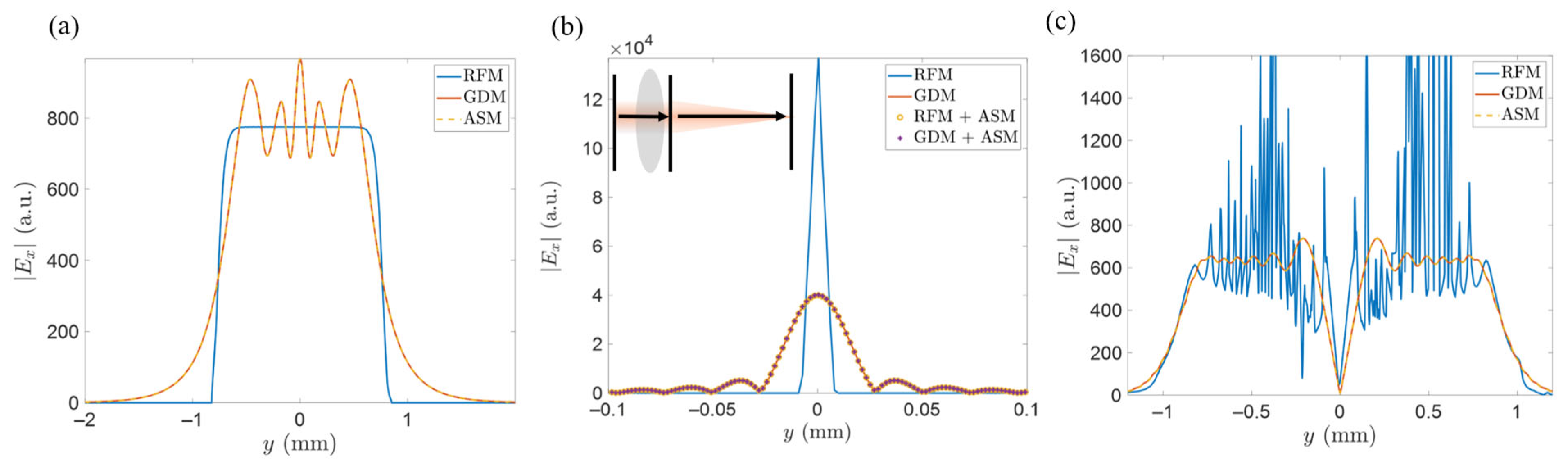
2.4. Comparison to Ray-Field Method

As noted at the start of Section 2.3, GDM is considered to provide greater accuracy than RFM. In the following sections, we first present an overview of RFM, including a generalization to account for ray polarization. This is followed by a comparison of the two methods to justify this accuracy claim.

Similar to the GDM, RFM involves decomposing an input field component $U_{\mathrm{in}}$ into a set of rays with directions determined from Equation (7). While the GDM uses Gaussian beams with finite width, the RFM assumes pencil rays throughout such that ray polarization at a point $r_{i\mathrm{n}}$ on the input plane is directly determined from the input field at that point:

$$E_{\mathrm{in}}\left(r_{\mathrm{in}}\right)=\{\begin{array}{cc}{E}_{x,\mathrm{in}}\left(r_{\mathrm{in}}\right)\widehat{x}-{\displaystyle \frac{k_{x,\mathrm{in}}{E}_{x,\mathrm{in}}\left(r_{\mathrm{in}}\right)}{k_{z,\mathrm{in}}}}\widehat{z} & \mathrm{for} U_{\mathrm{in}}:=E_{x,\mathrm{in}}\\ E_{y,\mathrm{in}}\left(r_{\mathrm{in}}\right)\widehat{y}-{\displaystyle \frac{k_{y,\mathrm{in}}{E}_{y,\mathrm{in}}\left(r_{\mathrm{in}}\right)}{k_{z,\mathrm{in}}}}\widehat{z} & \mathrm{for} U_{\mathrm{in}}:=E_{y,\mathrm{in}}\end{array}.$$

(50)

Furthermore, RFM does not consider ray path diffraction, and ray data including position, density, and optical path length are integrated to determine the output field. For a ray traced to output plane with position $r_{\mathrm{out}}$, the RFM gives the field at that point as

$$E_{\mathrm{out}}\left(r_{\mathrm{out}}\right)=\alpha \exp \left(i{k}_0\mathrm{OPL}\right)P{E}_{\mathrm{in}}\left(r_{\mathrm{in}}\right),$$

(51)

where OPL and P is optical path length and polarization raytracing matrix of a ray from input plane to output plane, respectively; α is a geometrical factor to ensure energy conservation, and is given as [25]

$$\alpha =\sqrt{{\displaystyle \prod }_{i=1}^N{\displaystyle \frac{{\widehat{k}}_i\cdot {\widehat{n}}_i}{{\widehat{k}}_{i-1}\cdot {\widehat{n}}_i}}{\displaystyle \frac{W_{\mathrm{in}}{\widehat{k}}_{\mathrm{in}}\cdot \widehat{z}}{W_{\mathrm{out}}{\widehat{k}}_{\mathrm{out}}\cdot \widehat{z}}}},$$

(52)

with ${\widehat{k}}_i$ and ${\widehat{n}}_i$ being ray direction after and surface normal at the i-th surface, respectively; The product of sequence is over all surfaces in between the input and output planes; W_in and $W_{\mathrm{out}}$ are effective cross sections subtended by a ray on the input and output planes, respectively. In practice, these cross sections are calculated by creating parabasal rays in addition to a given base ray under consideration. For N base rays with positions $r_{\mathrm{in}}$ on the input plane, Equation (51) provides output fields only at the corresponding positions $r_{\mathrm{out}}$ of each base ray. To calculate the output field at arbitrary locations, scattered interpolation is necessary to estimate values between these defined points.

While having a much simpler formalism than GDM, RFM is suitable primarily for beams that: (1) propagate over short distances such that path diffraction can be ignored, (2) are located away from foci and optical caustics where geometrical intensity law is not violated (i.e., $W_{\mathrm{out}}$ in Equation (52) is not close to zero), and (3) have relatively simple wavefronts such that base ray patterns remain stable during propagation so scattered interpolation can be applied. Some numerical experiments are presented below to illustrate these limitations.

We first examine the free-space propagation of a x-polarized super-Gaussian beam over a distance of 15 mm, comparing results obtained from three methods: ASM, RFM, and GDM. The ASM result is considered the ground truth. Here, we set the beam wavelength to 4 μm and its radius to 1 mm. Figure 6a presents a comparison of the output beam’s y-slices from each method. Over longer distances, diffraction effects become more pronounced. The GDM result closely resembles the ASM result, which suggests that GDM effectively accounts for ray path diffraction. In contrast, the RFM does not reflect changes in the beam profile with propagation distance, as it does not consider diffraction effects, resulting in an unchanged output beam profile in comparison to the input one. The discrepancy between the RFM and ASM/GDM results highlights the limitations of RFM for simulating long-distance propagation.

Next, we examine the propagation of the same super-Gaussian beam through a singlet, illustrated schematically in the inset of Figure 6b. The singlet has radii of curvature $R_1=-R_2=20 \mathrm{mm}$, a thickness of 5 mm, a refractive index of 2, and its front surface positioned 3 mm after the input plane. We consider the singlet to have an ideal coating that is infinitely thin and provides perfect transmission at each surface. Propagation can be conducted in two ways: (1) a single-step approach, where the input beam is directly propagated to the rear focal plane using either RFM or GDM; or (2) a two-step approach, where the input beam is first propagated to a plane immediately following the singlet using either method, then the resulting field is relayed to the rear focal plane using the ASM.

The y-slices of the output beams on the rear focal plane for each approach are compared in Figure 6b, revealing some key observations. Both the GDM single-step and the two-step approach combining GDM and ASM produce highly similar results, closely resembling an Airy pattern. This similarity suggests that GDM, whether alone or combined with ASM, effectively captures diffraction effects. In practice, the two-step approach is more efficient, as the down-sampling strategy for GDM (Equation (49)) can be applied at the output plane after the singlet but cannot be applied in the single-step approach, where the field is evaluated directly near a focus. Thus, we generally use the ASM to propagate a field to its focus for the design examples in Section 3.

Meanwhile, the two-step approach with RFM and ASM yields comparable results, as the short propagation distance the RFM involved minimizes the impact of diffraction. However, the single-step RFM approach produces an unrealistic result near the focal region, where diffraction effects become significant and cannot be neglected. This example highlights the limitations of RFM in simulating beam behavior in regions of strong focus.

The final experiment examines the propagation of an optical vortex beam in free space. The beam parameters are consistent with those used in the previous examples, with the addition that the beam is left circularly polarized and has a topological charge of +1 on the input plane. Figure 6c presents the y-slices at the output plane, located 10 mm beyond the input plane. In this figure, results from the GDM closely match those from the ASM, which can be considered as the ground truth. A clear minimum can be observed on the optical axis, which is a key feature for optical vortex beams. In Section 3, we will further demonstrate propagation of an optical vortex beam through refractive optics. Meanwhile, the RFM introduces significant errors due to the optical vortex beam’s complex, helical wavefront. This wavefront causes substantial spatial variation in the base ray pattern during propagation, resulting in notable errors from the scattered interpolation required in RFM.

These experiments validate that, while the formalism for GDM is more complex than RFM, it provides reliable accuracy for simulating the propagation of complex beams through refractive optics and is an integral part of this work for physical optics modeling of MS-refractive hybrid lenses.

2.5. Propagation Through Metasurfaces

Up to this point, we have discussed propagators for simulating field propagation through free space and refractive optics. Next, we need a method to model the interaction between a transmissive MS and an incoming field. Our discussion is limited to MSs with a fixed, subwavelength pitch size for meta-atoms across the entire surface, excluding pure freeform MSs. The transmitted field from such an MS can be engineered by designing the nanostructures of the meta-atoms in each unit cell.

While full-wave simulations of MSs offer a more rigorous approach, they often suffer from long computational times or impractical simulation sizes, particularly for large-scale MS designs. A common method for modeling macroscale MS response is to utilize the inherent properties of subwavelength meta-atoms, a technique known as the LUA, frequently used in MS designs [34,35,36,37]. This method simulates a single meta-atom unit cell replicated infinitely in the x-y plane via periodic boundary conditions, as illustrated by the cross-section in Figure 7a; the simulation volume is denoted by input/output planes and dot black lines showing the sides with periodic boundary conditions. Under the LUA, each meta-atom is treated as if surrounded by an infinite array of identical meta-atoms and has been shown to provide a good approximation for slowly varying phase profiles [38]. LUA response to incident plane waves can be simulated through RCWA, which rigorously solves Maxwell’s equations for a 2D periodic array. Polarization-dependent transmission coefficients (including amplitude and phase) can be estimated using RCWA. This method inherently neglects near-field coupling between disparate meta-atoms. Although more advanced methods exist [39,40,41,42], they fall beyond the scope of this work. It is important to note, however, that LUA remains a widely adopted method in many MS design studies due to its balance between simplicity and effectiveness.

The core principles of RCWA and its numerical implementation are well documented in the literature [43], and we provide a concise introduction here relevant to our discussion. For more in-depth treatment, we refer interested readers to the original references. Consider a plane wave with polarization $E_{\mathrm{in}}=E_{x,\mathrm{in}}\widehat{x}+E_{y,\mathrm{in}}\widehat{y}+E_{z,\mathrm{in}}\widehat{z}$ launched from the input region of a meta-atom periodic array with a propagation direction ${\widehat{k}}_{\mathrm{in}}=k_{x,\mathrm{in}}\widehat{x}+k_{y,\mathrm{in}}\widehat{y}+k_{z,\mathrm{in}}\widehat{z}$. The plane of polarization must be orthogonal to the propagation direction such that ${\widehat{k}}_{\mathrm{in}}\cdot E_{\mathrm{in}}=0$. Thus, for a given ${\widehat{k}}_{\mathrm{in}}$, we can use two electric field components to uniquely specify input polarization while the third component can be calculated from the orthogonality condition. We choose the x- and y-directions to specify an input polarization, which conforms to the model we had in Section 2.1.

For a specified meta-atom structure and incident wave vector ${\widehat{k}}_{\mathrm{in}}$, the primary outcome from RCWA is the transmission coefficients. These coefficients establish a relationship between the input field components and the resulting output field components:

$$\left[\begin{array}{c}{E}_{x,\mathrm{out}}\\ E_{y,\mathrm{out}}\end{array}\right]=\left[\begin{array}{cc}{t}_{xx}& t_{xy}\\ t_{yx}& t_{yy}\end{array}\right] \left[\begin{array}{c}{E}_{x,\mathrm{in}}\\ E_{y,\mathrm{in}}\end{array}\right].$$

(53)

Due to the linearity of Maxwell’s equations (assuming all materials are linear), the overall output field from a meta-atom can be interpreted as a superposition of output fields from different input polarization components. As a consequence, to obtain matrix elements $t_{xx}$ and $t_{yx}$, we launch an input plane wave with polarization:

$$E_{\mathrm{in}}^{\left(x\right)}=\widehat{x}-{\displaystyle \frac{k_{x,\mathrm{in}}}{k_{z,\mathrm{in}}}}\widehat{z}.$$

(54)

Note it has a unity x-component, and the z-component can be determined from the incident wave vector. For a subwavelength meta-atom structure, we only need to consider the zero-order transmitted field [38], which gives $t_{xx}$ and $t_{yx}$ as its field components such that

$$E_{\mathrm{out}}^{\left(x\right)}=t_{xx}\widehat{x}+t_{yx}\widehat{y}+E_z^{\left(x\right)}\widehat{z}.$$

(55)

A similar expression also exists for reflections, but this work focuses solely on transmissive meta-atoms. We can get the other two matrix elements, $t_{xy}$ and $t_{yy}$, by exciting the meta-atom with another input plane with polarization:

$$E_{\mathrm{in}}^{\left(y\right)}=\widehat{y}-{\displaystyle \frac{k_{y,\mathrm{in}}}{k_{z,\mathrm{in}}}}\widehat{z},$$

(56)

which gives zero-order transmitted field:

$$E_{\mathrm{out}}^{\left(y\right)}=t_{xy}\widehat{x}+t_{yy}\widehat{y}+E_z^{\left(y\right)}\widehat{z}.$$

(57)

Typically, it is not needed to record the transmitted electric field z-component, as it can be obtained from the orthogonality condition ${\widehat{k}}_{\mathrm{out}}\cdot E_{\mathrm{out}}=0$ on demand. It should be noted that the matrix elements determined in this manner are complex transmission coefficients that account for amplitude and phase change, and also any potential impedance mismatch between the input and output regions due to material differences.

Considering, as an example, an MS that is formed from meta-atoms in Figure 7b. The only free parameter for this polarization-insensitive meta-atom is the hole radius R, also indicated in the figure. Thus, an MS built on this meta-atom structure has a radius $R\left(x, y\right)$ for each meta-atom site (x, y) across the aperture. We refer to a specific arrangement $R\left(x, y\right)$ as a layout and this can be designed to provide optimal spatial modulation of phase across the aperture. To optimize a layout, we need to expediently generate output fields given an arbitrary input field and this needs to be done across the whole aperture with varying meta-atoms. To do so, we pre-compile a multi-dimensional database spanning meta-atom radii, incident angles, wavelengths, and polarizations. This mapping of local input fields to local output fields between the two planes is computed in the LUA using RCWA following Equation (53) and is used as a look-up table during optimization.

Figure 7c,d display two matrix elements, $t_{xx}$ and $t_{xy}$, from a database at a wavelength of 4 μm. Since the meta-atom is designed to be polarization-insensitive, the off-diagonal element $t_{xy}$ has a significantly smaller magnitude compared to the diagonal element $t_{xx}$ at small incident zenith angles and shows only weak dependence on the incident azimuthal angle. Due to the symmetry of the meta-atom, the remaining two matrix elements exhibit similar behavior.

With a meta-atom polarization database, simple steps can be followed to estimate the output field $E_{x\left(y\right),\mathrm{out}}\left(x, y\right)$ after an MS when an input field $E_{x\left(y\right),\mathrm{in}}\left(x, y\right)$ is specified. Since the two input field components are generally independent, these steps have to be performed separately. Taking $E_{x,\mathrm{in}}\left(x, y\right)$ for example, Equation (7) can be used to find local wave vector ${\widehat{k}}_{\mathrm{in}}\left(x, y\right)$. Next, we convert wave vector components to incident zenith and azimuthal angles as

$$\theta \left(x,y\right)={\cos }^{-1}\left(k_{z,\mathrm{in}}\left(x,y\right)\right),$$

(58a)

$$\varphi \left(x,y\right)={\tan }^{-1}\left({\displaystyle \frac{k_{y,\mathrm{in}}\left(x,y\right)}{k_{x,\mathrm{in}}\left(x,y\right)}}\right).$$

(58b)

Given $R\left(x, y\right), \theta \left(x,y\right), \varphi \left(x,y\right)$, and the input field wavelength, we can compute the output field (Figure 7a). First, we sample the input field at each meta-atom site to compute the amplitude and orientation of an x-polarized plane wave approximating the local input field at that site. We apply an interpolation to the meta-atom polarization database to obtain transmission matrix elements $t_{xx}\left(x, y\right)$ and $t_{yx}\left(x, y\right)$ across the aperture. This is repeated for $E_{y,\mathrm{in}}\left(x, y\right)$ to obtain $t_{xy}\left(x, y\right)$ and $t_{yy}\left(x, y\right)$. Finally, Equation (53) can be used to obtain $E_{x\left(y\right),\mathrm{out}}\left(x, y\right)$. This approach implies that the finest resolution for fields across a MS is determined by the pitch of individual meta-atom. As the meta-atoms are subwavelength in size, only the zero-order transmission mode exists, resulting in the field being considered to be locally homogeneous within each meta-atom pitch [38].

Another commonly-seen category of MS utilizes geometric phase to control polarized wavefront. Figure 8a shows an archetypal anisotropic meta-atom design, where the pillar rotation angle, ${\theta }_r\left(x, y\right)$, can be rotated across the MS plane to control the phase applied to the input field. To model this type of MS, we construct a meta-atom polarization database similar to the one described before, but including a parameter sweep over ${\theta }_r$ (Figure 8b).

Furthermore, we can make use of the geometric phase relation to reduce simulation load:

$$\left[\begin{array}{cc}{t}_{xx}& t_{xy}\\ t_{yx}& t_{yy}\end{array}\right]\approx \left[\begin{array}{cc} \cos {\theta }_r& -\sin {\theta }_r\\ \sin {\theta }_r& \cos {\theta }_r\end{array}\right]\left[\begin{array}{cc}{t}_{xx}^{\left(0\right)}& 0\\ 0& t_{yy}^{\left(0\right)}\end{array}\right]\left[\begin{array}{cc} \cos {\theta }_r& \sin {\theta }_r\\ -\sin {\theta }_r& \cos {\theta }_r\end{array}\right] ,$$

(59)

where the principal transmission coefficients, $t_{xx}^{\left(0\right)}$ and $t_{yy}^{\left(0\right)}$, are rigorously simulated in RCWA with ${\theta }_r=0$ for on-axis, crossed linear polarizations as inputs. Equation (59) is generally sufficient for paraxial incident angles and suffices for several design examples in the following section. When large incident angles are present, a comprehensive database should be constructed rigorously to account for non-paraxial effects. Figure 8b shows the $t_{xx}$ component is uniform for input (air) angles < 30$°$; beyond that the approximation in Equation (59) breaks down for this particular meta-atom basis.

3. Design Examples

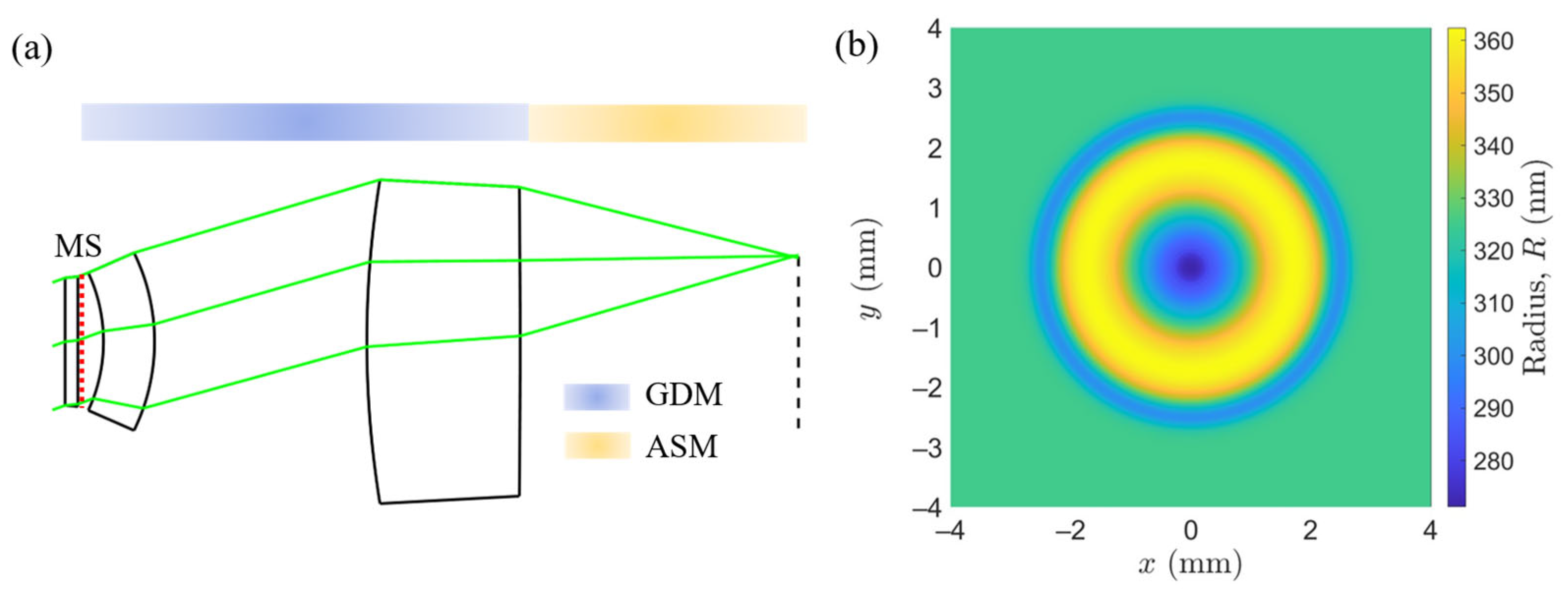
3.1. Hybrid Lens with Aberration-Correcting Metasurface

The first example examines a hybrid lens that incorporates an MS aberration corrector. A range of optical systems employing MSs for aberration correction have been documented in the literature, with MS wavefront correction achievable through optical design software like Zemax [15,21], theoretical optimization [17], or inverse designs [24].

As depicted in Figure 9a, we consider a configuration in which an MS is positioned in the object space of an F/2, 40° field-of-view (FOV), 10-mm effective focal length (EFL) lens, comprising two germanium refractive elements. We assume an ideal anti-reflection coating on all refractive surfaces. The MS is based on the polarization-insensitive meta-atom design in Figure 7b, and its meta-atom radius layout $R\left(x, y\right)$, shown in Figure 9b, has been optimized through an inverse design process to correct aberrations across the FOV in the mid-wave infrared (MWIR) range [18]. The MS is added to correct aberrations without carrying much optical power so that a slowly-varying radius layout is achieved.

To evaluate the performance of optimized hybrid lenses, a point spread function (PSF) calculation is performed. An x-polarized, super Gaussian beam at the maximum field angle with a wavelength of 4 μm is prepared as the input field. To compare the PSFs of the lens with and without the MS, we employ a propagation scheme as illustrated in Figure 9a: the input field is propagated through the MS aberration corrector using the meta-atom polarization database; GDM then propagates the field through the two refractive optics, followed by the ASM to bring the field to the image plane. Note that the meta-atom polarization database already considers the presence of substrate, so the input field is prepared in the substrate when the MS aberration corrector is inserted. This example follows Reference [24] only now we are able to include vector fields and polarization.

Figure 10a–d show the field components on the image plane of the MS-refractive hybrid lens, along with the counterpart obtained using scalar field propagation, which was used in the design phase of the hybrid lens [24]. Figure 10e–h further display the corresponding results without the MS in place. From these figures, it is clear that the x-component dominates the field, with a pattern that closely resembles that observed under the scalar field approximation. This agreement indicates that the MS design is effectively polarization-insensitive, allowing it to be well-described by a scalar field model without significant polarization effects. The y-component remains relatively small because the system is polarization-insensitive. In contrast, the z-component becomes more prominent near focus due to the lens’s focusing effect, which naturally induces a longitudinal field component—especially for tightly focused beams, as is characteristic of high numerical aperture (NA) systems. Meanwhile, the inclusion of the MS significantly impacts the imaging performance, as evidenced by the smaller size of the PSF when the MS is presented. This improvement highlights the MS’s role in enhancing image quality by correcting aberrations from the refractive optics, and the ability of GDM to correctly capture small wavefront variations during its decomposition process. It should be mentioned this system could be simulated using the RFM described in Section 2.4 for propagation through refractive optics—since path diffraction effects across them are minimal and the wavefronts are relatively simple—the corresponding results obtained are included in the Supplementary Information Section S2.

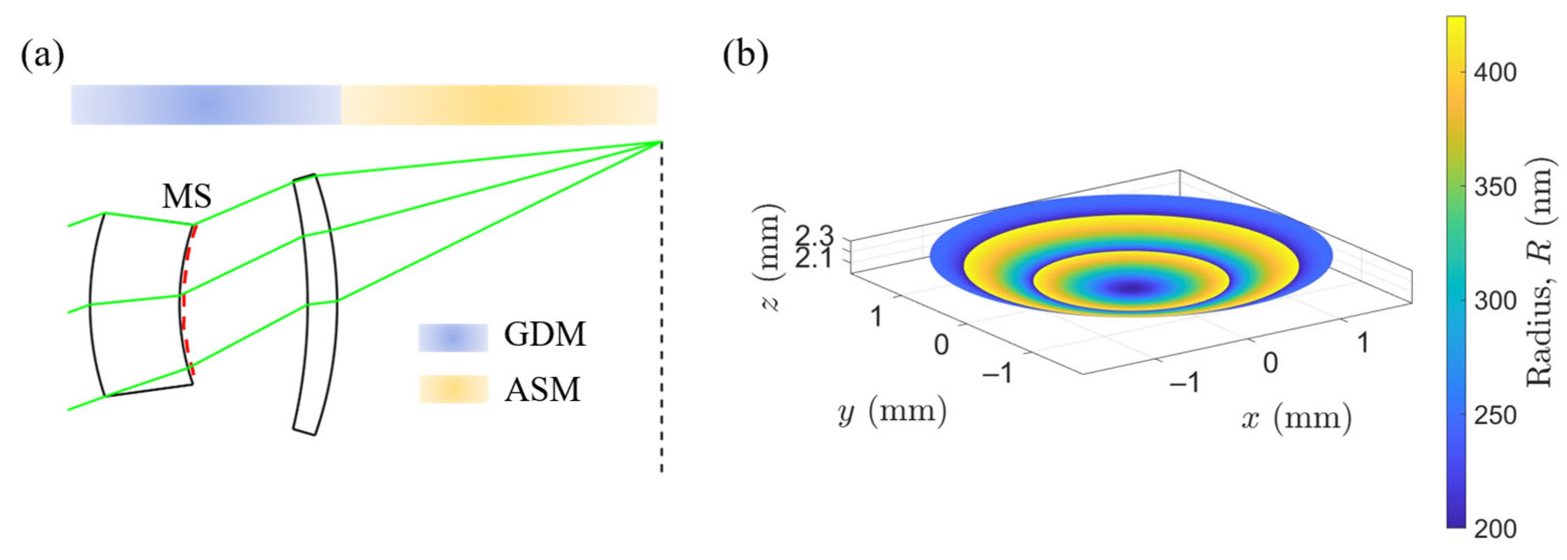
3.2. Hybrid Lens with a Curved Metasurface

While MSs are typically flat optics fabricated on planar substrates—leading to the wave-based propagation method outlined in Section 2.5—an alternative ray-based approach can be employed for MSs composed of polarization-insensitive meta-atoms (e.g., the hole meta-atoms in Figure 7b). This method, which is compatible with both GDM and RFM, modifies the underlying polarization raytracing to account for the MS response. Furthermore, the formulation can be extended to model propagation through a curved MS, which enables broader applicability in hybrid optical systems. The details of such generalization are given in the Supplementary Information, Section S3.

Figure 11a shows a hybrid lens with a curved MS. The F/2, 40° FOV, 10-mm EFL hybrid lens was optimized in Zemax, where the MS was initially treated as a parameterized phase surface and optimized alongside the refractive surfaces to minimize RMS spot sizes. After optimization, the phase profile at the central wavelength of 4 μm was mapped to a meta-atom hole layout, as shown in Figure 11b. To reduce surface reflections, a simple quarter-wave anti-reflection coating at 4 μm is applied to all refractive surfaces.

As in the previous example, an x-polarized super-Gaussian beam at the maximum field angle and a wavelength of 4 μm is used as the input field. The GDM is used to propagate the field through the two optics and is followed by the ASM to bring the field to the image plane. A comparison of PSFs with and without the MS is shown in Figure 12, showing the effectiveness of the MS.

It is important to note that the current implementation of curved MS modeling using either GDM or RFM is limited to polarization-insensitive MSs. For polarization-sensitive MSs, such as those based on geometric phase (e.g., Figure 8a), the meta-atoms induce polarization-dependent splitting, generating separate rays for different eigenpolarization states. Accurately modeling such behavior requires an extended framework capable of tracking child rays, which is beyond the scope of this work.

3.3. Focusing a Cylindrical Radially-Polarized Beam

In the previous examples, the systems have simple wavefronts with minimal polarization effects. To demonstrate the GDM can treat more complex wavefronts and provide full polarization tracking, we now consider a system illustrated in Figure 13a. An MS is positioned in front of a commercially available doublet lens (Thorlabs AC254-050-E) with diffraction-limited image quality. The MS is specifically designed to transform a homogeneous input beam into a radially polarized beam, which is subsequently focused by the doublet lens. This example was selected for the following reasons: (1) the complex beam profile after the MS prohibits the use of the simpler RFM; (2) near focus the PSF has a distinctive polarization structure due to the radially polarized input resulting in a strong, localized longitudinal component—a behavior not observed with homogeneously polarized beams [44]; (3) it enables a comparison with a semi-analytical model, offering additional validation of the accuracy of GDM, and (4) the generation and manipulation of vectorial.

An axial, x-polarized, super-Gaussian beam with a 3-mm-radius is positioned just before the MS; the wavelength is 4 μm. The MS is composed of anisotropic meta-atoms, as shown in Figure 8a, with a rotation angle layout ${\theta }_r\left(x, y\right)={\displaystyle \frac{1}{2}}{\tan }^{-1}{\displaystyle \frac{y}{x}}$. This layout imparts the desired radial polarization to the beam. Note that an azimuthally polarized beam would be generated instead if the input beam were y-polarized. This meta-atom is optimized at a wavelength of 4 μm and is intended to convert the hardness of circularly polarized light along the optical axis. The meta-atom polarization database in Figure 8b is utilized to obtain the transmitted field components after the MS. The propagation steps proceed as follows: the field is first propagated through the MS to a plane immediately in front of the doublet lens using the ASM; The GDM is then employed to simulate propagation through the doublet lens, after which ASM is used again to focus the beam to the image plane of the hybrid lens.

Figure 13b,c illustrate the x-component of the field before and after the doublet lens, respectively. Despite the beam’s highly inhomogeneous profile, it is effectively managed by the GDM with adaptive beam widths. Figure 13d presents y-slices of the field components at the image plane of the hybrid lens, where a cylindrical coordinate system is applied. The radial component displays the characteristic donut shape, while a compact longitudinal component is also observed—both are features of a radially polarized beam near focus [44].

In this example, we consider an on-axis, x-polarized input beam to demonstrate the functionality of the hybrid lens. For completeness, an additional case involving an on-axis, y-polarized input beam is presented in the Supplementary Information, Section S4, where the hybrid lens produces an azimuthally polarized focused beam. Furthermore, to highlight the generality of the proposed method, we also investigate the system’s response under off-axis incidence.

Since the doublet lens in the system is diffraction-limited, it can be substituted by an equivalent thin lens at its image space principal plane, as illustrated in Figure 14a. In this thin lens model, the polarization effect across the lens is assumed to be ideal and treated geometrically, as detailed in the Supplementary Information, Section S4. By applying the ASM for all propagation steps in this model, we obtain the resultant PSF shown in Figure 14b, which can be directly compared with the realistic setup (Figure 13d). Minor deviations are largely due to polarization differences propagating through the real doublet lens versus the idealized thin lens. Despite these differences, the close resemblance between the two PSFs strongly validates the reliability of the GDM approach for MS-refractive hybrid lens simulations. It is noted that the thin lens model is designed to have an ideal phase profile at the target wavelength of 4 μm. However, it can introduce defocus at other wavelengths, in contrast to the achromatic off-the-shelf doublet lens, which better maintains focus across a broader spectral range.

3.4. Adjoint Gradient Optimization

Inverse design has emerged as a powerful tool to optimize MSs down to the individual meta-atoms placed across the aperture. It works by starting with an objective function and computationally refining meta-atom geometries or layouts to approach that objective. By iteratively adjusting design parameters, the inverse design achieves control over optical properties such as phase, amplitude, and polarization modulation. This approach has proven effective for creating MSs that enable aberration correction [45], amplitude control [46], and multifunctional beam manipulation [47].

To highlight the utility of the ray-wave method in MS inverse design, we present a design example of an MS-refractive hybrid lens optimized through the adjoint gradient method (AGM)—a subset of inverse design techniques. AGM leverages both forward and backward wave propagation: the input beam propagates forward through the system, while an adjoint field propagates backward from a target plane. By analyzing both fields collectively, we compute the gradient of the objective function with respect to the MS parameters, enabling optimization of the MS layout. This example highlights how physical optics techniques, such as the ASM and GDM, can be integrated with adjoint optimization for polarization-sensitive MS designs within hybrid lenses. Surprisingly, these physical optics techniques work for adjoint fields which are not real electromagnetic fields and do not strictly obey Maxwell’s Equations; however, some considerations on bounds, stability, convergence, and energy conservation need to be made.

Consider a system illustrated in Figure 15a, which consists of an MS placed just before a germanium double-convex lens with an EFL of 5.15 mm. Ideal coating is assumed on both surfaces of the lens. This MS-refractive hybrid lens is designed to asymmetrically separate two input fields, each with a homogeneous polarization and a radius of 0.7 mm. The input polarization states are $J=\widehat{x}+\sqrt{2}\left(1+i\right)\widehat{y}$ and its orthogonal state $J_{\perp }$. As the fields propagate through the system, each incident polarization state is converted into its complex conjugate ($J^{*}$ and $J_{\perp }^{*}$, respectively). These converted states are spatially separated and focused onto an image plane positioned 1 mm beyond the focal plane of the refractive lens, enabling polarization conversion, spatial separation, and focusing in a single system. Notably, the deliberate positioning of the image plane beyond the lens focal plane requires the MS to impart additional optical power and the two targeted positions on the image plane are also purposefully made asymmetric, emphasizing the flexibility of MSs and optimization via AGM.

We make some simplifying assumptions to streamline the example, but all these can be treated more rigorously as discussed in Section 2. We consider on-axis incident light and use Equation (59) to describe the interaction of the MS with incident fields. We treat the principal transmission coefficients, $t_{xx}^{\left(0\right)}$ and $t_{yy}^{\left(0\right)}$, and rotation angles ${\theta }_r$ across the MS as free parameters to be optimized by the AGM; this by-passes pre-compiling an LUA database but introduces risk that certain combinations of $t_{xx}^{\left(0\right)}$, $t_{yy}^{\left(0\right)}$ and ${\theta }_r$ may not be realizable in a given meta-atom basis. Further, the MS is assumed to function through phase modulation alone, meaning that each transmission coefficient takes the form $t_{xx}^{\left(0\right)}=\exp \left(i{\varphi }_{xx}^{\left(0\right)}\right)$ and similarly for $t_{yy}^{\left(0\right)}$; This yields phase control without altering amplitude. The detailed formulation of AGM is provided in Supplementary Information, Section S5, while the following provides an outline of key steps in the MS optimization process.

For each input field, an adjoint field representing the target beam profile is defined on a plane immediately after the lens, as labeled in Figure 15a. Taking the incident state $J$ as an example, the adjoint field is set with a spherical wavefront centered at the target point on the image plane, with its profile illustrated in Figure 15b. The GDM is then employed to propagate this adjoint field backward through the lens, as shown in Figure 15c, followed by ASM propagation to the MS plane. With both the incident and adjoint field profiles across the MS calculated, iterative updates to the MS parameters can be made such that the transmitted field after the MS has maximized resemblance to the adjoint field. In practice, the orthogonal input state $J_{\perp }$ requires a similar adjoint field setup, and the AGM uses both sets of fields to optimize MS parameters jointly.

In this example, the adjoint field only has to be determined and propagated to the backside of the MS a single time; no changes to the backward propagation occur during MS optimization. Similarly, the input field is only computed once. The techniques, nonetheless, are robust and fast enough to support more complicated system optimizations such as co-optimizing refractive elements and/or optimizing with multiple MSs.

An objective function is defined as the mean of the inner products between the transmitted fields (obtained after the MS) and their corresponding adjoint fields at each iteration, normalized by the adjoint field magnitude. As shown in Figure 16a, this metric tracks convergence during the iterative optimization, offering a quantitative measure of agreement between the transmitted and adjoint field profiles as the MS parameters are updated. A value of unity indicates perfect agreement. The final objective function value of 0.9850 demonstrates the effectiveness of the AGM in achieving the desired transformation. A similar analysis can be performed on the target plane in Figure 15a, given a value of 0.9642.

Figure 16b shows the optimized phase layout ${\varphi }_{xx}^{\left(0\right)}$ from the AGM, revealing a complex, asymmetric pattern necessary for the MS to achieve the specified functionalities. While the layout of the other two MS parameters exhibits similar characteristics. Once the MS is optimized, forward propagation of the input fields through the system yields the PSFs on the image plane, as shown in Figure 16c,d. Each output field is projected onto the designated conjugate polarization states $J^{*}$ and $J_{\perp }^{*}$, confirming that the system achieves the targeted spatial separation for the two orthogonal states, as specified in Figure 15a.

Finally, it is important to note that adjoint fields, though mathematically constructed to reflect the system’s desired functionalities, can still be effectively propagated using AGM and GDM, provided that these functionalities can be expressed as smooth field profiles. This ensures that adjoint fields align with physically viable solutions, facilitating efficient convergence toward the desired MS design within a physical optics framework.

3.5. Full-Stokes Polarization Sensing

In this section, we present a final design example: a full-Stokes polarization camera that can sense the polarization state of a scene. This example is chosen to demonstrate the capability of the GDM in modeling refractive lenses with relatively complex geometries. As illustrated in Figure 17a, the system comprises an MS-refractive hybrid lens designed for polarization sensing. The primary refractive lens is an F/2, 3-mm EFL system with a 60° FOV. Its role is to focus and separate incoming fields from various field angles, while the MS, positioned near the image plane, is used to analyze the polarization states of the focused fields.

The primary lens system consists of four refractive elements and a separate stop. To ensure high image quality across the FOV, the final element in the lens is aspherical. The system is optimized for operation at a wavelength of 4 μm with diffraction-limited image quality across the FOV and a small distortion (<2%). Quarter-wave anti-reflection coating is applied to all refractive surfaces. The paraxial assumption will be made such that Equation (59) can be used to calculate transmissions across the MS. Consequently, the primary lens is further designed to be telecentric in image space. This ensures that the chief ray angle remains small across the FOV, resulting in converging beams near the focal point having axes as parallel to the optical axis as possible. Such a configuration supports accurate polarization analysis while maintaining spatial resolution.

The GDM is implemented to propagate incident fields to a plane immediately in front of the MS. The primary lens separates fields from different incident angles while preserving the polarization state of the scene. Meanwhile, the MS functions as a polarization splitter. Referring to Figure 17b, a converging field after the primary lens passes through the MS, which analyzes the polarization state of the field and sorts it into four quadrants on the super-pixel. Each quadrant corresponds to an analyzing polarization state $J_i$, i = {1, 2, 3, 4}, chosen to be the vertices of a regular tetrahedron inscribed in the Poincaré sphere. This configuration maximizes the sensitivity of the polarization analysis device [48].

As with the previous example, the MS is modeled as lossless and defined by three parameters: ${\varphi }_{xx}^{\left(0\right)}$, ${\varphi }_{yy}^{\left(0\right)}$, and ${\theta }_r$. Once the primary lens design is fixed and the four analyzing polarization states are defined, the MS can be designed following the strategy outlined in Supplementary Information, Section S6. As an example, Figure 17c illustrates the layout for ${\varphi }_{xx}^{\left(0\right)}$ within a super-cell. The ASM is used to propagate the field after the MS to the image plane. By examining the intensity distribution across a super-pixel, the polarization state of the incoming field can be reconstructed.

For example, when the incident field has a left-circular polarization state $J_1$, the z-component of the electric field after the primary lens, simulated using the GDM, is shown in Figure 18a. The spiral pattern indicates it stays left-circular polarized after propagation. After propagating through the MS to the image plane, this field produces the intensity distribution in Figure 18b. Four distinct spots are observed, with the brightest in the first quadrant corresponding to $J_1$. Energy still appears in other quadrants as the MS design must account for multiple polarization states during optimization. Using the measured quadrant powers $P={\left[\begin{array}{cc}{P}_1& \begin{array}{cc}{P}_2& \begin{array}{cc}{P}_3& P_4\end{array}\end{array}\end{array}\right]}^T$ in a super-pixel, a device matrix B (see the Supplementary Information, Section S6) can reconstruct the incident Stokes vector $S=BP$. Here, the device matrix is calibrated solely for on-axis incidence. Figure 18c shows good agreement between the predicted and ground truth polarization ellipses. Similar analyses for other incident polarizations, such as the state orthogonal to $J_3$, also confirm the system’s ability to analyze polarization states accurately (Figure 18d–f).

However, accuracy degrades for off-axis fields at larger field angles, as the field after the primary lens diverges from the symmetric spherical wavefront assumed in the MS design. Figure 19 shows that at half field (15°), the system can still reliably estimate polarization, but at full field (30°), noticeable deviations from the ground truth occur. Despite these limitations, it should be emphasized that the ray-wave hybrid propagation method can be used to estimate system performance beyond idealized on-axis conditions. This approach enables comprehensive evaluations that support further improvements. For instance, the primary lens design could constrain the ray cone shapes to remain symmetric across the FOV, and an angular-dependent device matrix could account for variations in beam shape (Figure S7).

4. Discussions

To the best of our knowledge, this is the first work that presents a transparent discussion on strategies for physical optics modeling of MS-refractive hybrid lenses, where full-wave solvers are computationally impractical. Our proposed model extends beyond traditional raytracing by employing a ray-wave hybrid scheme, enabling the analysis of electromagnetic field distributions at any plane within a hybrid lens. While the concept of ray-wave hybridization has been explored in prior literature [24,25], existing approaches are often limited—either relying on the simplified RFM discussed in Section 2.4 or assuming scalar wave approximations that neglect complex wavefront and polarization evolution. Full-path vectorial diffraction calculations based on the chirp z-transform have also been proposed for efficiently simulating complex optical systems [49]. However, these approaches typically assume ideal lenses that strictly obey Abbe’s sine condition. As a result, lens-induced polarization effects are idealized, and aberrations are not accounted for. In contrast, the method introduced in this work provides a more generalized and physically rigorous framework that captures vectorial field behavior in real, non-ideal lenses, including polarization effects and aberrations across the entire system.

We believe this framework will contribute meaningfully to the advancement of modeling, simulation, and even inverse optimization of MS-refractive hybrid lenses. Although this work focuses on transmissive systems, it can be readily extended to reflective optics such as mirrors or reflective MSs by (1) incorporating mirror reflection coefficients into the polarization raytracing matrix (Equation (43)) and (2) modeling reflective metasurface responses via zero-order reflection coefficients, as described in the meta-atom polarization database (Equation (53)). Also, the proposed method could potentially be used to simulate systems with other diffractive optics, such as holograms, and can benefit from computational imaging algorithms [50] to fulfill high-fidelity imaging.

The design examples presented in the prior section demonstrate the effectiveness of the proposed method. However, there are assumptions that should be acknowledged. Central to this work is the use of the LUA for simulating largescale MS responses. An important assumption underlying this approach is that meta-atom near-field effects are neglected. These non-local effects may become more significant in MSs that are functionally dependent on resonances [51], characterized by a freeform topology [52], or exhibit rapid variations in meta-atom geometry relative to the wavelength. To accurately capture the coupling effects in such non-local metasurfaces, full-wave electromagnetic solvers, such as the FDFD method, can be employed for smaller MS apertures. Alternatively, several more efficient methods for capturing these coupling effects have been proposed in the literature, such as using a global statistical learning optimization approach to optimize 2D resonant MSs while accounting for coupling effects [51], applying coupled mode theory to design propagation phase-based MSs by modeling the meta-atoms as truncated waveguides [42], or leveraging deep learning techniques to estimate the near-field interactions based on the meta-atom and its neighboring elements [39]. Another approach involves decomposing the MS into overlapping domains and applying full-wave simulations to each domain individually [41]. In principle, these advanced methods could replace the meta-atom look-up table approach outlined in Section 2.5 and could also be integrated with the GDM and ASM to provide a more accurate simulation of MS-refractive hybrid lenses.

Further, this work focuses on developing numerical methods to model and design MS-refractive optics. While experimental validation is not presented at the current stage, to ensure the validity of the proposed method, we conduct data-driven analyses such as verifying energy conservation across perfectly anti-reflective coated refractive optics and in free space. Also, in Section 3.3, the thin-lens model, which can be simulated simply using the ASM, is used to ensure the GDM calculation is physically sound. Furthermore, for designs such as the MS aberration corrector in Section 3.1, we demonstrated our modulation transfer function (MTF) calculation result (following Reference [24]) closely matches those generated by Zemax, providing additional confidence in the modeling accuracy. These steps, while not direct experimental validation, collectively indicate that the proposed method offers physically sound and reliable predictions for practical optical system design.

5. Conclusions

This work presents a ray-wave hybrid framework for simulating and designing MS-refractive hybrid optical systems. It introduces computationally light and rigorous physical optics modeling of wave propagation and polarization effects in such systems. Central to this framework is the GDM, which enables efficient and accurate modeling of wavefront propagation through hybrid systems by bridging the gap between ray-based and wave-based approaches. The GDM is particularly advantageous for hybrid designs, as it provides high precision in the analysis of polarization and optical aberrations while maintaining computational efficiency.

We demonstrated the versatility of this approach through several design examples. These include the optimization of MSs for aberration correction, focusing a radially polarized beam, spatial separation of polarization states with asymmetric focusing, and the design of a full-Stokes polarization camera leveraging the complex geometry of a multi-element refractive lens. These examples illustrate the capability of the proposed method to accommodate varying degrees of complexity in hybrid systems, including polarization manipulation and integration with advanced refractive optics. An example presented also highlights the power of adjoint gradient optimization when combined with the GDM and ASM. This combination enables efficient optimization over MS parameters, facilitating designs that meet performance criteria defined as an objective function.

The proposed method could be improved in several ways. While this study employed the LUA for MS modeling, its limitations, such as neglecting near-field interactions, were acknowledged. Future extensions to include advanced near-field modeling could refine simulation accuracy further. For example, with a meta-atom polarization database having angular responses, a two-dimensional discrete-space impulse response can be used to map fields across an MS [40]. Meanwhile, a fixed Gaussian pattern is assumed in the GDM. Adaptive decomposition processes [53], which determine the best positions to place Gaussian beams, can be adopted to further reduce decomposition error and/or boost speed. While the GDM considers path diffraction, edge diffraction is not considered in our implementation because we clip entire Gaussian beamlets when an aperture is encountered; this could be improved, for example, by resampling fields at limiting apertures using truncated Gaussian beams at the edge as proposed in Reference [32].

References

1. Safaei, A.; Vázquez-Guardado, A.; Franklin, D.; Leuenberger, M.N.; Chanda, D. High Efficiency Broadband Mid-infrared Flat Lens. Adv. Optical Mater. 2018, 6, 1800216. [Google Scholar] [CrossRef]
2. Chen, W.-T.; Zhu, A.Y.; Sisler, J.; Bharwani, Z.; Capasso, F. A Broadband Achromatic Polarization-insensitive Metalens Consisting of Anisotropic Nanostructures. Nat. Commun. 2019, 10, 355. [Google Scholar] [CrossRef] [PubMed]
3. Shrestha, S.; Overvig, A.C.; Lu, M.; Stein, A.; Yu, N.-F. Broadband Achromatic Dielectric Metalenses. Light Sci. Appl. 2018, 7, 85. [Google Scholar] [CrossRef]
4. Zhou, H.-P.; Chen, L.; Shen, F.; Guo, K.; Guo, Z.-Y. Broadband Achromatic Metalens in the Midinfrared Range. Phys. Rev. Appl. 2019, 11, 024066. [Google Scholar] [CrossRef]
5. Hu, S.; Wei, L.; Long, Y.; Huang, S.; Dai, B.; Qiu, L.; Zhuang, S.; Zhang, D. Longitudinal Polarization Manipulation Based on All-Dielectric Terahertz Metasurfaces. Opt. Express 2024, 32, 6963–6976. [Google Scholar] [CrossRef]
6. Wang, B.; Dong, F.; Feng, H.; Yang, D.; Song, Z.; Xu, L.; Chu, W.; Gong, Q.; Li, Y. Rochon-Prism-Like Planar Circularly Polarized Beam Splitters Based on Dielectric Metasurfaces. ACS Photonics 2018, 5, 1660–1664. [Google Scholar] [CrossRef]
7. Zhang, F.; Yu, H.; Fang, J.; Zhang, M.; Chen, S.; Wang, J.; He, A.; Chen, J. Efficient Generation and Tight Focusing of Radially Polarized Beam from Linearly Polarized Beam with All-Dielectric Metasurface. Opt. Express 2016, 24, 6656–6664. [Google Scholar] [CrossRef]
8. Zhang, B.; Hu, Z.; Wang, J.; Wu, J.; Tian, S. Creating Perfect Composite Vortex Beams with a Single All-Dielectric Geometric Metasurface. Opt. Express 2022, 30, 40231–40242. [Google Scholar] [CrossRef]
9. Zang, H.; Zhou, X.; Yang, Z.; Yu, Q.; Zheng, C.; Yao, J. Polarization Multiplexed Multifunctional Metasurface for Generating Longitudinally Evolving Vector Vortex Beams. Phys. Lett. A 2024, 497, 129336. [Google Scholar] [CrossRef]
10. Huo, P.; Zhang, C.; Zhu, W.; Liu, M.; Zhang, S.; Zhang, S.; Chen, L.; Lezec, H.J.; Agrawal, A.; Lu, Y.; et al. Photonic Spin-Multiplexing Metasurface for Switchable Spiral Phase Contrast Imaging. Nano Lett. 2020, 20, 2791–2798. [Google Scholar] [CrossRef]
11. Wen, D.; Yue, F.; Ardron, M.; Chen, X. Multifunctional Metasurface Lens for Imaging and Fourier Transform. Sci. Rep. 2016, 6, 27628. [Google Scholar] [CrossRef]
12. Ge, S.; Li, X.; Liu, Z.; Zhao, J.; Wang, W.; Li, S.; Zhang, W. Polarization-Multiplexed Metasurface Enabled Tri-Functional Imaging. Opt. Lett. 2023, 48, 5683–5686. [Google Scholar] [CrossRef]
13. Zheng, C.L.; Ni, P.N.; Xie, Y.Y.; Genevet, P. On-Chip Light Control of Semiconductor Optoelectronic Devices Using Integrated Metasurfaces. Opto-Electron. Adv. 2025, 8, 240159. [Google Scholar] [CrossRef]
14. Fu, P.; Ni, P.-N.; Wu, B.; Pei, X.-Z.; Wang, Q.-H.; Chen, P.-P.; Xu, C.; Kan, Q.; Chu, W.-G.; Xie, Y.-Y. Metasurface Enabled On-Chip Generation and Manipulation of Vector Beams from Vertical Cavity Surface-Emitting Lasers. Adv. Mater. 2022, 34, 202204286. [Google Scholar] [CrossRef] [PubMed]
15. Chen, W.-T.; Zhu, A.Y.; Sisler, J.; Huang, Y.-W.; Yousef, K.; Lee, E.; Qiu, C.-W.; Capasso, F. Broadband Achromatic Metasurface-Refractive Optics. Nano Lett. 2018, 18, 7801–7808. [Google Scholar] [CrossRef] [PubMed]
16. Hu, T.; Wang, S.; Wei, Y.; Wen, L.; Feng, X.; Yang, Z.; Zheng, J.; Zhao, M. Design of a Centimeter-Scale Achromatic Hybrid Metalens with Polarization Insensitivity in the Visible. Opt. Lett. 2023, 48, 1898–1901. [Google Scholar] [CrossRef]
17. Sawant, R.; Andrén, D.; Martins, R.J.; Khadir, S.; Verre, R.; Käll, M.; Genevet, P. Aberration-Corrected Large-Scale Hybrid Metalenses. Optica 2021, 8, 1405–1411. [Google Scholar] [CrossRef]
18. Chu, Y.; Xiao, X.; Ye, X.; Chen, C.; Zhu, S.; Li, T. Design of Achromatic Hybrid Metalens with Secondary Spectrum Correction. Opt. Express 2023, 31, 21399–21406. [Google Scholar] [CrossRef]
19. Liu, M.; Zhao, W.; Wang, Y.; Huo, P.; Zhang, H.; Lu, Y.-Q.; Xu, T. Achromatic and Coma-Corrected Hybrid Meta-Optics for High-Performance Thermal Imaging. Nano Lett. 2024, 24, 7609–7615. [Google Scholar] [CrossRef]
20. Thomas, S.; George, J.G.; Ferranti, F.; Bhattacharya, S. Metaoptics for Aberration Correction in Microendoscopy. Opt. Express 2024, 32, 9686–9698. [Google Scholar] [CrossRef]
21. Cuillerier, A.C.; Borne, J.; Thibault, S. Fast Metasurface Hybrid Lens Design Using a Semi-Analytical Model. J. Opt. Soc. Am. B 2023, 40, 72–78. [Google Scholar] [CrossRef]
22. Chen, W.; Shih, K.-H.; Renshaw, C.K. Dispersive Sweatt Model for Broadband Lens Design with Metasurfaces. Photonics 2025, 12, 43. [Google Scholar] [CrossRef]
23. Ding, Y.; Stone, B.D.; Bahl, M.; Heller, E.; Scarmozzino, R. Hybrid Refractive-Metalens Design for Imaging Applications. In Proceedings of the SPIE 12666, Current Developments in Lens Design and Optical Engineering XXIV, San Diego, CA, USA, 20–25 August 2023. [Google Scholar] [CrossRef]
24. Shih, K.-H.; Renshaw, C.K. Hybrid Meta/Refractive Lens Design with an Inverse Design Using Physical Optics. Appl. Opt. 2024, 63, 4032–4043. [Google Scholar] [CrossRef] [PubMed]
25. Wyrowski, F.; Kuhn, M. Introduction to Field Tracing. J. Modern Opt. 2010, 58, 449–466. [Google Scholar] [CrossRef]
26. Ashcraft, J.N.; Douglas, E.S.; Kim, D.; Riggs, A.J.E. Hybrid Propagation Physics for the Design and Modeling of Astronomical Observatories: A Coronagraphic Example. J. Astron. Telesc. Instrum. Syst. 2023, 9, 048003. [Google Scholar] [CrossRef]
27. Worku, N.G.; Hambach, R.; Gross, H. Decomposition of a Field with Smooth Wavefront into a Set of Gaussian Beams with Non-Zero Curvatures. J. Opt. Soc. Am. A 2018, 35, 1091–1102. [Google Scholar] [CrossRef]
28. Harvey, J.E.; Irvin, R.G.; Pfisterer, R.N. Modeling Physical Optics Phenomena by Complex Ray Tracing. Opt. Eng. 2015, 54, 035105. [Google Scholar] [CrossRef]
29. Bergbauer, S.; Pollard, D.D. How to Calculate Normal Curvatures of Sampled Geological Surfaces. J. Struct. Geol. 2003, 25, 277–289. [Google Scholar] [CrossRef]
30. McCartin, B.J. A Matrix Analytic Approach to Conjugate Diameters of an Ellipse. Appl. Math. Sci. 2013, 7, 1797–1810. [Google Scholar] [CrossRef]
31. Yun, G.; Crabtree, K.; Chipman, R.A. Three-Dimensional Polarization Ray-Tracing Calculus I: Definition and Diattenuation. Appl. Opt. 2011, 50, 2855–2865. [Google Scholar] [CrossRef]
32. Worku, N.G.; Gross, H. Propagation of Truncated Gaussian Beams and Their Application in Modeling Sharp-Edge Diffraction. J. Opt. Soc. Am. A 2019, 36, 859–868. [Google Scholar] [CrossRef]
33. Luce, A.; Mahdavi, A.; Marquardt, F.; Wankerl, H. TMM-Fast, a Transfer Matrix Computation Package for Multilayer Thin-Film Optimization: Tutorial. J. Opt. Soc. Am. A 2022, 39, 1007–1013. [Google Scholar] [CrossRef] [PubMed]
34. Shalaginov, M.Y.; An, S.-S.; Yang, F.; Su, P.; Lyzwa, D.; Agarwal, A.M.; Zhang, H.-L.; Hu, J.-J.; Gu, T. Single-Element Diffraction-Limited Fisheye Metalens. Nano Lett. 2020, 20, 7429–7437. [Google Scholar] [CrossRef]
35. Fan, C.-Y.; Lin, C.-P.; Su, G.-D.J. Ultrawide-Angle and High-Efficiency Metalens in Hexagonal Arrangement. Sci. Rep. 2020, 10, 15677. [Google Scholar] [CrossRef] [PubMed]
36. Arbabi, A.; Arbabi, E.; Kamali, S.M.; Horie, Y.; Han, S.; Faraon, A. Miniature Optical Planar Camera Based on a Wide-Angle Metasurface Doublet Corrected for Monochromatic Aberrations. Nat. Commun. 2016, 7, 13682. [Google Scholar] [CrossRef] [PubMed]
37. Groever, B.; Chen, W.-T.; Capasso, F. Meta-Lens Doublet in the Visible Region. Nano Lett. 2017, 17, 4902–4907. [Google Scholar] [CrossRef]
38. Pestourie, R.; Pérez-Arancibia, C.; Lin, Z.; Shin, W.; Capasso, F.; Johnson, S.G. Inverse Design of Large-Area Metasurfaces. Opt. Express 2018, 26, 33732–33747. [Google Scholar] [CrossRef]
39. An, S.; Zheng, B.; Shalaginov, M.Y.; Tang, H.; Li, H.; Zhou, L.; Dong, Y.; Haerinia, M.; Agarwal, A.M.; Rivero-Baleine, C.; et al. Deep Convolutional Neural Networks to Predict Mutual Coupling Effects in Metasurfaces. Adv. Opt. Mater. 2022, 10, 2102113. [Google Scholar] [CrossRef]
40. Torfeh, M.; Arbabi, A. Modeling Metasurfaces Using Discrete-Space Impulse Response Technique. ACS Photonics 2020, 7, 941–950. [Google Scholar] [CrossRef]
41. Lin, Z.; Johnson, S.G. Overlapping Domains for Topology Optimization of Large-Area Metasurfaces. Opt. Express 2019, 27, 32445–32453. [Google Scholar] [CrossRef]
42. Wu, Z.; Huang, X.; Yu, N.; Yu, Z. Inverse Design of a Dielectric Metasurface by the Spatial Coupled Mode Theory. ACS Photonics 2024, 11, 3019–3025. [Google Scholar] [CrossRef]
43. Rumpf, R.C. Improved Formulation of Scattering Matrices for Semi-Analytical Methods That Is Consistent with Convention. Prog. Electromagn. Res. B 2011, 35, 241–261. [Google Scholar] [CrossRef]
44. Zhan, Q.; Leger, J.R. Focus Shaping Using Cylindrical Vector Beams. Opt. Express 2002, 10, 324–331. [Google Scholar] [CrossRef] [PubMed]
45. Backer, A.S. Computational Inverse Design for Cascaded Systems of Metasurface Optics. Opt. Express 2019, 27, 30308–30331. [Google Scholar] [CrossRef]
46. Wang, Z.-Q.; Li, F.-J.; Deng, Q.-M.; Wan, Z.; Li, X.; Deng, Z.-L. Inverse-Designed Jones Matrix Metasurfaces for High-Performance Meta-Polarizers. Chin. Opt. Lett. 2024, 22, 023601. Available online: https://opg.optica.org/col/abstract.cfm?URI=col-22-2-023601 (accessed on 17 April 2025). [CrossRef]
47. Zheng, H.; He, M.; Zhou, Y.; Kravchenko, I.I.; Caldwell, J.D.; Valentine, J.G. Compound Meta-Optics for Complete and Lossless Field Control. ACS Nano 2022, 16, 15100–15107. [Google Scholar] [CrossRef]
48. Soma, G.; Komatsu, K.; Ren, C.; Nakano, Y.; Tanemura, T. Metasurface-Enabled Non-Orthogonal Four-Output Polarization Splitter for Non-Redundant Full-Stokes Imaging. Opt. Express 2024, 32, 34207–34222. [Google Scholar] [CrossRef]
49. Hu, Y.; Wang, Z.; Wang, X.; Ji, S.; Zhang, C.; Li, J.; Zhu, W.; Wu, D.; Chu, J. Efficient Full-Path Optical Calculation of Scalar and Vector Diffraction Using the Bluestein Method. Light Sci. Appl. 2020, 9, 119. [Google Scholar] [CrossRef]
50. Rosen, J.; Alford, S.; Allan, B.; Anand, V.; Arnon, S.; Arockiaraj, F.G.; Art, J.; Bai, B.; Balasubramaniam, G.M.; Birnbaum, T.; et al. Roadmap on Computational Methods in Optical Imaging and Holography [Invited]. Appl. Phys. B 2024, 130, 166. [Google Scholar] [CrossRef]
51. Isnard, E.; Héron, S.; Lanteri, S.; Elsawy, M. Advancing Wavefront Shaping with Resonant Nonlocal Metasurfaces: Beyond the Limitations of Lookup Tables. Sci. Rep. 2024, 14, 1555. [Google Scholar] [CrossRef]
52. Chung, H.; Miller, O.D. High-NA Achromatic Metalenses by Inverse Design. Opt. Express 2020, 28, 6945–6965. [Google Scholar] [CrossRef] [PubMed]
53. Xia, D.; Ma, L.; Bai, M.; Shao, X. Fast Algorithm of Arbitrary Beam Propagation Based on Adaptive Elliptical Gaussian Beam Decomposition. In Proceedings of the 2019 International Applied Computational Electromagnetics Society Symposium (ACES), Miami, FL, USA, 14–19 April 2019; Available online: https://ieeexplore.ieee.org/document/8712898 (accessed on 15 April 2025).
Figure 1. Schematic diagram for an MS-refractive hybrid lens. A vector field is sequentially propagated through the optical elements until the image plane using suitable physical optics propagators.
Photonics 12 00401 g001
Figure 2. Illustrations for Gaussian decomposition process. (a) Individual Gaussian beam is prepared on the input plane with center position r in and direction k ^ in . Input transverse planes Pin are defined to be transversal to k ^ in . Among them, the one intersects r in is the principal input transverse plane Pin,0. (b) Principal directions, s ^ in and p ^ in , for a Gaussian beam are defined on Pin,0 and serve as a convenient basis to described the Gaussian beam in local coordinate system. (c) Projections of amplitude covariance matrix principal axes, e 1 and e 2 , onto Pin,0 give a pair of conjugated axes, e 1 and e 2 , which define an ellipse on Pin,0 with principal axes being p 1 and p 2 .
Photonics 12 00401 g002
Figure 3. Illustrations for Gaussian differential raytracing. A base ray (shown in red) on the input plane is accompanied by four parabasal rays (with only two depicted in the figure). These rays are traced to the output region, where their positions and directions are utilized to compute the transfer matrix Mc for the base ray from the principal input transverse plane Pin,0 to the principal output transverse plane Pout,0.
Photonics 12 00401 g003
Figure 4. Illustration for Gaussian beam superposition on the output plane. To determine the field contribution of a Gaussian beam at a query point ro, a free space transfer matrix Mout is constructed, and the phase accumulated along the ray path is also accounted for.
Photonics 12 00401 g004
Figure 5. Flowchart for Gaussian decomposition method.
Photonics 12 00401 g005
Figure 6. Comparison y-slices of output field x-component from various propagators for (a) free space propagation of a super-Gaussian beam, (b) propagation of a super-Gaussian beam through a singlet to its rear focal plane, and (c) free space propagation of an optical vortex beam.
Photonics 12 00401 g006
Figure 7. (a) Illustration of an MS composed of hole meta-atoms. The local response of the MS is modeled from meta-atom response under the LUA. A single meta-atom is highlighted, whose response can be simulated by the RCWA. (b) Unit-cell for Polarization-insensitive hole meta-atom to control wavefront by varying its hole radius, R. Amplitude for transmission matrix elements (c) txx and (d) txy as functions of incidence zenith angle in air θ air , incidence azimuthal angle ϕ, and hole radius R at a wavelength of 4 μm.
Photonics 12 00401 g007
Figure 8. (a) Anisotropic meta-atom with a pillar for geometric phase modulation. (b) Amplitude for transmission matrix element txx as functions of incidence zenith angle in air θ air , incidence azimuthal angle ϕ, and pillar orientation angle θr at a wavelength of 4 μm. The remaining three matrix elements have similar behaviors.
Photonics 12 00401 g008
Figure 9. (a) A MS-refractive hybrid lens with an MS located in front of a refractive lens for aberration correction. Sections with different propagators are indicated, along with chief and marginal rays for a 20° field. (b) Meta-atom hole radius layout on the MS.
Photonics 12 00401 g009
Figure 10. (ac) Magnitude of electric field components on the image plane of the MS-refractive hybrid lens in Figure 9a, and (d) is the corresponding scalar field magnitude. (eh) are the corresponding results when the MS in the hybrid lens was removed.
Photonics 12 00401 g010
Figure 11. (a) An MS-refractive hybrid lens with a curved MS. Sections using different propagators are indicated, along with chief and marginal rays for a 20° field. (b) Meta-atom hole radius layout on the curved MS.
Photonics 12 00401 g011
Figure 12. (a,b) Magnitude of electric field transverse components on the image plane of the MS-refractive hybrid lens in Figure 11a. (c,d) are the corresponding results when the MS in the hybrid lens was removed.
Photonics 12 00401 g012
Figure 13. (a) An MS-refractive hybrid lens with an MS located in front of a doublet lens for radially polarized beam focusing. Sections using different propagators are indicated, along with chief and marginal rays for an on-axis field. (b,c) Real part of electric field x-component in front of and after the doublet lens, respectively. (d) Magnitude of beam cylindrical component y-slices on the image plane.
Photonics 12 00401 g013
Figure 14. (a) Thin lens model for the hybrid lens in Figure 13a. The ASM is used for propagation. Chief and marginal rays for an on-axis field are shown. (b) Magnitude of beam cylindrical component y-slices on the image plane.
Photonics 12 00401 g014
Figure 15. (a) Illustration for adjoint gradient optimization for a polarization-splitting hybrid lens. Sections using different propagators are indicated. (b) Real part of the x-component of the adjoint field defined on the target plane for incident polarization state J and (c) its backward propagation through the lens.
Photonics 12 00401 g015
Figure 16. (a) Evolution of objective function for the adjoint gradient optimization. (b) Optimized MS layout for ϕ x x ( 0 ) . (c,d) PSFs on the image plane for incident polarization states J and J , respectively.
Photonics 12 00401 g016
Figure 17. (a) Illustration for an MS-refractive hybrid lens consists of a primary lens and a polarization-splitting MS. Sections using different propagators are indicated, along with chief and marginal rays for a 30° field. (b) A converging beam after the primary lens is passed through a super-cell on the MS and the power is sorted to the four quadrants on the sensor super-pixel. (c) MS super-cell layout for ϕ x x ( 0 ) .
Photonics 12 00401 g017
Figure 18. (a) The real part of electric field z-component after the primary lens, (b) the z-component Poynting vector on the image plane, and (c) comparison of polarization ellipses between the estimated polarization state (blue) and the ground truth (red) under an incident polarization J1. (df) are the corresponding results under an incident polarization that is orthogonal to J3.
Photonics 12 00401 g018
Figure 19. Comparisons of Stokes vectors for the detected states (blue) and the incident states (red) for an incident angle of (a) 15° and (b) 30°.
Photonics 12 00401 g019