On a Different Vision of Kerr Law in Nonlinear Optical Waveguide Theory

Abstract

This paper focuses on electromagnetic transverse-electric wave propagation in a planar shielded waveguide filled with nonlinear medium. Instead of using the standard local Kerr (cubic) nonlinearity, we suggest a (nonlocal) modification of this law. In comparison with the standard formula, this modification does not produce infinitely many nonperturbative guided modes. In this research, we present the dispersion equation for propagation constants, eigenwaves and propagation constants via explicit formulas. The found results are compared with the ones relating to the corresponding linear problem and the nonlinear one with the classical Kerr’s law. Numerical results are also presented and discussed.

1. Introduction

Local Kerr law (or cubic nonlinearity) is one of the most important nonlinearities in the field of nonlinear optics [1,2,3,4,5]. This nonlinearity corresponds to the so-called self-action effects, where the nonlinearity does not affect the frequency of the electromagnetic wave [6,7,8,9,10,11]. This nonlinearity is observed in medium with inversion center under sufficiently powerful electromagnetic wave [11,12,13].

This paper introduces the modified Kerr law, which is nonlocal, and studies its influence on the propagation of monochromatic transverse-electric (TE) electromagnetic waves in a plane dielectric layer having such nonlinear permittivity. The introduced dependence is different from the standard one and is described in detail below.

We work with Maxwell’s equation in the harmonic mode

$$rot\mathbf{H}=-i\omega ϵ\mathbf{E},rot\mathbf{E}=i\omega \mu \mathbf{H},$$

(1)

where $ϵ$ and $\mu$ are the permittivity and permeability of the medium.

The standard way of introducing the local Kerr nonlinearity is the series expansion of the polarization vector with truncating of higher-order terms (which is possible under specific physical restrictions) and then substituting the resulting relation into the Maxwell equations. Going the standard way, researchers obtain the Kerr nonlinearity in the form

$$ϵ={ϵ}_l+a{\left|\mathbf{E}\right|}^2,$$

(2)

where ${ϵ}_l$ is a linear part of the permittivity and a is a coefficient of the nonlinearity; both parameters are assumed to be positive constants, and $\mathbf{E}$ is the electric field used in (1) (see, for example, [2,5,11,13]).

One of the interesting and intriguing results obtained for problems of monochromatic wave propagation in plane dielectric waveguides filled with Kerr media (2) is that there arise infinitely many nonperturbative guided modes [14]. We note that existence of infinitely many nonperturbative solutions was theoretically proved for a wide range of waveguiding problems; see the Kerr case for TE-waves in open [14,15] and shielded [16] waveguides, for transverse-magnetic (TM) waves in open [17,18] and shielded [19] waveguides and also the case of polynomial and power nonlinearities for TE- [20,21] and TM-waves [22,23]. We also note that there is at least one more alternative approach presented in [24,25].

To be more precise, using Formula (2), one obtains infinitely many eigenvalues (propagation constants) that we denote by ${\lambda }_n$, where $n=1,2,\dots$ and ${\lambda }_n\to +\infty$ as $n\to \infty$, and infinitely many eigenfunctions (eigenwaves) ${\mathbf{E}}_n$ corresponding to ${\lambda }_n$. We stress that ${\mathbf{E}}_n$ depends on spatial coordinates over the domain, coefficient a and ${\lambda }_n$. Due to the results proved in [16,26,27], we clarify that there are two important facts: the first one is that $max|{\mathbf{E}}_n|\to +\infty$ as ${\lambda }_n\to +\infty$; the second one is that for any nonperturbative eigenwave $u_n$, it is true that $max|{\mathbf{E}}_n|\to +\infty$ as $a\to +0$. We stress that for any finite ${\lambda }_n$, and any positive a, the corresponding eigenwave ${\mathbf{E}}_n$ is a vector-bounded function; see Section 3.4 for rigorous formulations.

The mathematical reason for infinitely many nonperturbative solutions arising is that the Kerr law in the form (2) is an unbounded function (it increases unboundedly as $\left|\mathbf{E}\right|$ increases unboundedly). It is clear that that the field does not increase unboundedly in the waveguiding system. However, for any prescribed value, there are eigenmodes with larger maximums. In addition, the real existence of infinitely many guided waves does not look physically realistic. Due to the above-mentioned behavior, it seems reasonable to consider alternative approaches to study Kerr nonlinearity.

In this paper, we suggest the following nonlinear dependence for the Kerr nonlinearity

$$ϵ={ϵ}_l+b\int {\left|\mathbf{E}\right|}^{2}dx$$

(3)

with the same notation as above, where the dimension of b equals the dimension of $a/h$, and the integration is taken over that domain in which the problem is considered (in the case of a plane waveguide, the integration is taken over the transverse coordinate). This nonlinear law, on the one hand, results in a finite number of solutions. On the other hand, we do not change Formula (2) by a saturated nonlinearity that is a bounded function of $\left|\mathbf{E}\right|$ for all $\left|\mathbf{E}\right|$; see, for example, [28,29,30,31]. It is true that ${\int \left|\mathbf{E}\right|}^2$ is not necessary finite, as $\mathbf{E}\to \infty$; however, it turns out that in comparison with the above-described case, in such nonlinear law, the field stays bounded for any possible b and $\lambda$, where $\lambda$ is a propagation constant. The main disadvantage of our approach is that we no longer have nonperturbative solutions, which are interesting both from mathematical and physical points of view.

Thus, in this paper, we suggest the modified Kerr law and study its influence on the problem of a TE-wave propagation in a plane shielded waveguide. Together with analytical study, numerical results and comparison with previous results are presented.

After this introduction, let us consider a monochromatic TE wave

$$\mathbf{E}{e}^{-i\omega t}=e^{-i\omega t}{(0,{\mathcal{E}}_y,0)}^{\top },\mathbf{H}{e}^{-i\omega t}=e^{-i\omega t}{({\mathcal{H}}_x,0,{\mathcal{H}}_z)}^{\top },$$

(4)

where

$${\mathcal{E}}_y=E_y(x;\gamma )e^{i\gamma z},{\mathcal{H}}_x=H_x(x;\gamma )e^{i\gamma z},{\mathcal{H}}_z=H_z(x;\gamma )e^{i\gamma z},$$

(5)

$\omega$ is a circular frequency, $\gamma$ is a real spectral parameter, which propagates in a planar shielded waveguide $\Sigma$ of thickness h filled with nonlinear medium having permittivity in the form (3). The waveguide $\Sigma$ is placed in Cartesian coordinates $Oxyz$; it is infinite along longitudinal axes $Oy$ and $Oz$ and is of finite thickness h along transverse axis $Ox$. The waveguide has infinitely conducted screens at the boundaries $x=0$ and $x=h$; see Figure 1. The permeability $\mu$ inside $\mathrm{\Sigma }$ is equal to the permeability of free space.

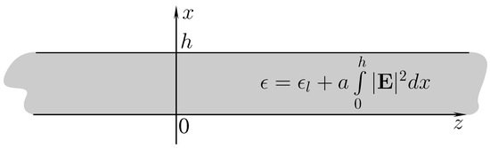
Figure 1. Geometry of the problem.

Inside the waveguide fields $\mathbf{E},the\mathbf{H}$ given in (4) and (5) satisfies Maxwell’s Equation (1). In addition, tangential components of the electric field vanish at the infinitely conducting screens, that is $E_y(0;\gamma )=E_y(h;\gamma )=0$. In addition, the quantity $E_y^{\prime }(0;\gamma )$ is assumed to be fixed and positive (below, we give comments about this condition).

Concluding this section, we briefly clarify why the considered problem admits only real $\gamma$ (propagation constants). In Formula (5), the functions $E_y$, $H_x$ and $H_z$ depend only on one spatial variable: transverse coordinate x. This choice of the fields is possible only in the case of real $\gamma$. Indeed, substituting fields $\mathbf{E}$ and $\mathbf{H}$ with Components (5) into Equation (1), we obtain resulting equations that depend on x and do not depend on z. To be more precise, multiplier $e^{i\gamma z}$ is reduced on both sides of the equations, and the term $\left|\mathbf{E}\right|$ does not depend on z as $|e^{i\gamma z}|=1$ for real $\gamma$. At the same time, if $\gamma$ is not real, then $|e^{i\gamma z}|$ is a function with respect to z. This means that components $E_y$, $H_x$ and $H_z$ depend not only on x but also on z. This contradicts the choice of these components as functions depending only on x. All this, however, does not mean that it is not possible to consider complex $\gamma$ in a waveguiding problem with Kerr nonlinearity. We just say that for complex $\gamma$, the problem cannot be solved mathematically correctly for Fields (4) and (5).

2. Materials and Methods

Although the paper focuses on the analytical study of the problem, some numerical results are presented as well; see Section 3.5. The description of numerical methods used in this study is given in Section 3.5. All numerical methods are implemented with the package <<Maple>>.

3. Results

3.1. Mathematical Statement of the Nonlinear Problem

Let us consider the equation

$$u^{″}\left(x\right)=-({\epsilon }_l-\lambda )u\left(x\right)-\alpha \left(\underset{0}{\overset{h}{\int }}{u}^2\left(t\right)dt\right)u\left(x\right),$$

(6)

where $x\in [0,h]$, $u\equiv u(x;\lambda )$ is a sought-for function, $\alpha$ and $\epsilon$ are positive constants and $\lambda$ is a real parameter, together with boundary conditions

$$\begin{array}{cc}\hfill u\left(0\right)& =0,u\left(h\right)=0,\hfill \end{array}$$

(7)

$$\begin{array}{cc}\hfill u^{\prime }\left(0\right)& =A,\hfill \end{array}$$

(8)

where A is an arbitrary positive constant.

We note that substituting Fields (4)–(5) into Maxwell’s Equation (1) and using notation $u:=E_y(x;\gamma )$, $\lambda :={\gamma }^2$, ${\epsilon }_l:={\omega }^2\mu {ϵ}_l$, $\alpha :={\omega }^2\mu b$, we obtain Equation (6). Thus, Equation (6) depends on frequency, as terms ${\epsilon }_l$ and $\alpha$ depend on $\omega$. We stress that the same notation is used in the problems below. From the conditions imposed on the electromagnetic field, one obtains Conditions (7) and (8).

Thus, our main goal is to study problem $\mathcal{Q}$, which is to find $\lambda =\widehat{\lambda }$ such that there exists solution $u(x;\widehat{\lambda })\in C^2[0,h]$ to Equation (6), satisfying Conditions (7) and (8).

Definition 1.

A value $\widehat{\lambda }$ such that there exists solution $u(x;\widehat{\lambda })\in C^2[0,h]$ to Equation (6), satisfying conditions (7) and (8), is called an eigenvalue, and the corresponding function $u(x;\widehat{\lambda })$ is called an eigenfunction of problem $\mathcal{Q}$.

So, the problem of electromagnetic wave propagation is equivalent to problem $\mathcal{Q}$, and therefore eigenvalues of problem $\mathcal{Q}$ are (squared) propagation constants of waveguide $\Sigma$. We stress, however, that due to the fact that $\gamma$ is real, and notation $\lambda :={\gamma }^2$, only positive eigenvalues of problem $\mathcal{Q}$ have electromagnetic sense. The same is also true for the linearized problem described in the next section.

3.2. Linearized Problem

Setting $\alpha =0$ in Equation (6), problem $\mathcal{Q}$ degenerates into a linear problem, which we call problem ${\mathcal{Q}}_0$.

Problem${\mathcal{Q}}_0$ is to find $\lambda =\tilde{\lambda }$ such that there exists a nontrivial function $v(x;\tilde{\lambda })\in C^2[0,h]$ satisfying the equation

$$v^{″}\left(x\right)=-({\epsilon }_l-\lambda )v\left(x\right)$$

(9)

and boundary conditions

$$v\left(0\right)=0,v\left(h\right)=0.$$

(10)

As is known, two boundary conditions are necessary and sufficient to obtain a uniquely defined discrete set of eigenvalues in an eigenvalue problem for a linear second-order differential equation; for this reason, Condition (8) is odd here. However, two Conditions (7) are not sufficient to obtain a uniquely define discrete eigenvalues in an eigenvalue problem for a nonlinear eigenvalue problem for a second-order differential equation. This is the reason to impose an additional condition. As such additional condition, we use Condition (8).

The following result takes place.

Theorem 1.

Problem ${\mathcal{Q}}_0$ has a finite number of positive and infinitely many number of negative eigenvalues $\lambda ={\tilde{\lambda }}_n$, defined by formula

$${\tilde{\lambda }}_n={\epsilon }_l-\frac{{\pi }^2{n}^2}{h^2};$$

(11)

the eigenfunction of problem ${\mathcal{Q}}_0$ corresponding to eigenvalue ${\tilde{\lambda }}_n$ is defined by the formula

$$v_n\left(x\right)=Bsin\frac{\pi nx}{h},$$

(12)

where B is an arbitrary nonzero constant.

As we explained above, from the electromagnetic standpoint, only positive $\tilde{\lambda }$ are interesting.

Corollary 1.

If positive eigenvalues $\lambda =\tilde{\lambda }$ of problem ${\mathcal{Q}}_0$ exist, then $\tilde{\lambda }\in (0,{\epsilon }_l)$.

The proof of this result is elementary and well-known and, for this reason, is omitted.

Numerical results for problem ${\mathcal{Q}}_0$ see in Figure 2 in Section 3.5.

3.3. Solvability of Problem Q

Let us assume that the solution to Equation (6) satisfying Condition (7) exists globally on the whole segment $x\in [0,h]$; the validity of this assumption is approved below. Then, integral ${\int }_0^h{u}^2\left(t\right)dt$ exists and, in fact, it is a positive parameter. Taking this into account, Equation (6) can be considered as an ordinary linear differential equation with constant coefficients; we can write its solution in the form

$$u\left(x\right)=C_{1}cos\left(x\sqrt{{\epsilon }_l-\lambda +\alpha {\int }_0^h{u}^2\left(t\right)dt}\right)+C_{2}sin\left(x\sqrt{{\epsilon }_l-\lambda +\alpha {\int }_0^h{u}^2\left(t\right)dt}\right),$$

where $C_1$ and $C_2$ are arbitrary constants.

Using boundary condition $u\left(0\right)=0$, one finds that $C_1=0$, and thus $u\left(x\right)$ can be rewritten as

$$u\left(x\right)=C_{2}sin\left(x\sqrt{{\epsilon }_l-\lambda +\alpha {\int }_0^h{u}^2\left(t\right)dt}\right).$$

(13)

Using condition $u\left(h\right)=0$, one obtains the equation

$$sin\left(h\sqrt{{\epsilon }_l-\lambda +\alpha {\int }_0^h{u}^2\left(t\right)dt}\right)=0.$$

(14)

In fact, this is the so-called dispersion equation, which defines propagation constants. Setting $\alpha =0$, one obtains the dispersion equation of the problem ${\mathcal{Q}}_0$.

Hence, one can see from (14) that

$${\epsilon }_l-\lambda +\alpha \underset{0}{\overset{h}{\int }}{u}^2\left(t\right)dt⩾0.$$

(15)

Indeed, as is known from the complex function theory, $sinz$ vanishes only for $z=\pi k$, $k\in \mathbb{Z}$. For this reason, the argument of sin in (14) must be real. Thus, Condition (15) is necessary.

From (14), one obtains

$${\epsilon }_l-\lambda +\alpha \underset{0}{\overset{h}{\int }}{u}^2\left(t\right)dt={\pi }^2{n}^2{h}^{-2},$$

(16)

where $n⩾1$ is an integer.

Substituting (16) into (13), solution $u\left(x\right)$ takes the form

$$u_n\left(x\right)=C_{2}sin\frac{\pi nx}{h}.$$

Using condition $u^{\prime }\left(0\right)=A$, one obtains

$$u_n\left(x\right)=\frac{hA}{\pi n}sin\frac{\pi nx}{h}.$$

(17)

Substituting (17) into Equation (16), one finds

$${\widehat{\lambda }}_n={\epsilon }_l+\frac{\alpha h^3{A}^2}{2{\pi }^2{n}^2}-\frac{{\pi }^2{n}^2}{h^2}.$$

(18)

So, one can see that for $\lambda ={\widehat{\lambda }}_n$, the corresponding function $u\equiv u_n\left(x\right)$ given by (17) satisfies Equation (6) and Conditions (7) and (8). It proves our assumption of the existence of a solution and, therefore, all further calculations are valid.

Values ${\widehat{\lambda }}_n$ are eigenvalues, and the corresponding functions $u_n\left(x\right)\equiv u(x;\widehat{\lambda })$ are eigenfunctions of problem $\mathcal{Q}$. One can see that Formulas (17) and (18) are explicit formulas for propagation constants and eigenwaves of problem $\mathcal{Q}$. One can also compare Formulas (11) and (12) for problem ${\mathcal{Q}}_0$ with similar Formulas (17) and (18) for problem $\mathcal{Q}$.

The following result takes place.

Theorem 2.

Problem $\mathcal{Q}$ has infinitely many negative and a finite number(possibly not one)of positive eigenvalues $\lambda ={\widehat{\lambda }}_n$; they are defined by Formula (18). In addition, it is true that

$$\underset{\alpha \to +0}{lim}{\widehat{\lambda }}_n={\tilde{\lambda }}_n,$$

(19)

where ${\tilde{\lambda }}_n$ are eigenvalues of (linear) problem ${\mathcal{Q}}_0$.

The eigenfunctions of problem $\mathcal{Q}$ are defined by Formula (17) and exactly coincide with the eigenfunctions of problem ${\mathcal{Q}}_0$, which are defined by Formula (12) provided that one set $B=B_n=\frac{hA}{\pi n}$ in (12).

Proof. 

The main part of the theorem easily results from Formula (18). Indeed, the first term is $O\left(1\right)$, the second one is $O\left(n^{-2}\right)$ and the third one is $O\left(n^2\right)$; in addition, the first two terms are positive, whereas the third one is negative. Then, there exists an integer $\widehat{n}$ such that for all $n⩾\widehat{n}$ the absolute value of the third term is larger than the sum of the first two terms. Thus, ${\widehat{\lambda }}_n>0$ for $n<\widehat{n}$ and ${\widehat{\lambda }}_n<0$ for $n⩾\widehat{n}$.

The link between solutions to the linear and nonlinear problems can be obtained passing to the limit $\alpha \to +0$ in Formula (18) and comparing the found expression with Formula (11), which defines the eigenvalues of problem ${\mathcal{Q}}_0$. □

From the electromagnetic standpoint, only positive $\widehat{\lambda }$ are interesting (the same is true for problem ${\mathcal{Q}}_0$). Then, the following corollary is a simple consequence of the found results.

Corollary 2.

If positive eigenvalues $\lambda =\widehat{\lambda }$ of problem $\mathcal{Q}$ exist, then $\tilde{\lambda }\in (0,{\epsilon }_l+\alpha t)$, where $t>0$ is a constant.

Numerical results for problem $\mathcal{Q}$ see in Figure 2, Figure 3, Figure 4, Figure 5, Figure 6 and Figure 7 in Section 3.5.

3.4. Problem ${\mathcal{Q}}^{\prime }$

In this section, we briefly present the main results in the case of monochromatic TE-wave propagation in a plane shielded dielectric layer filled with Kerr medium, where Kerr nonlinearity is described by Formula (2). This problem we denote problem ${\mathcal{Q}}^{\prime }$. In other words, the only difference between problems $\mathcal{Q}$ and ${\mathcal{Q}}^{\prime }$ is in the form of nonlinearity.

Problem ${\mathcal{Q}}^{\prime }$ is to find $\lambda ={\widehat{\lambda }}^{\prime }$ such that there exists function $w(x;{\widehat{\lambda }}^{\prime })\in C^2[0,h]$, which is the solution to equation

$$w^{″}=-({\epsilon }_l-\lambda )w\left(x\right)-\alpha w^3\left(x\right),$$

(20)

satisfying boundary conditions $w\left(0\right)=w\left(h\right)=0$ and $w^{\prime }\left(0\right)=A$, where A is an arbitrary positive constant. Problem ${\mathcal{Q}}^{\prime }$ is studied in [26,27].

For $\alpha =0$, problem ${\mathcal{Q}}^{\prime }$ degenerates into a linear one, which obviously coincides with problem ${\mathcal{Q}}_0$.

From a physical point of view, the positive eigenvalues $\lambda =\widehat{{\lambda }^{\prime }}$ of problem ${\mathcal{Q}}^{\prime }$ correspond to the so-called propagation constants of waveguide $\Sigma$ and the eigenfunctions $w\equiv w(x;\widehat{{\lambda }^{\prime }})$ correspond to the eigenmodes of the waveguide.

The following results take place [26,27].

Theorem 3.

Problem ${\mathcal{Q}}^{\prime }$ has infinitely many positive eigenvalues $\lambda =\widehat{{\lambda }^{\prime }}$ with an accumulation point at infinity for any $\alpha >0$.

This result means that there exist infinitely many eigenvalues $\lambda ={\widehat{{\lambda }^{\prime }}}_n>0$, where $n=1,2,\dots$, and eigenfunctions $w\equiv w_n$ of problem ${\mathcal{Q}}^{\prime }$ such that ${\widehat{{\lambda }^{\prime }}}_n\to +\infty$ as $n\to \infty$. We stress that even this result is completely different from those that are derived in problems ${\mathcal{Q}}_0$; see Theorem 1, Corollary 1 and $\mathcal{Q}$, as well as Theorem 2 and Corollary 2 and Figure 5 and Figure 7.

Theorem 4.

If problem ${\mathcal{Q}}_0$ has k eigenvalues $\lambda ={\tilde{\lambda }}_j$, where $j=1,\dots ,k$, then there are at least k eigenvalues $\lambda ={\widehat{{\lambda }^{\prime }}}_j$ of problem ${\mathcal{Q}}^{\prime }$ such that

$$\underset{\alpha \to +0}{lim}{\widehat{{\lambda }^{\prime }}}_j={\tilde{\lambda }}_j$$

(21)

for each j; in addition,

$$\underset{x\in (0,h)}{max}{w}^2(x;\widehat{{\lambda }^{\prime }})\to \infty \mathrm{as}\widehat{{\lambda }^{\prime }}\to +\infty .$$

(22)

We note that there is only a finite number of eigenvalues $\lambda =\widehat{{\lambda }^{\prime }}$ of problem ${\mathcal{Q}}^{\prime }$ satisfying Relation (21); see Figure 5 and Figure 7. This time again we pay attention to the difference between results found for problem ${\mathcal{Q}}^{\prime }$ and problems ${\mathcal{Q}}_0$ and $\mathcal{Q}$. To be more precise, in problems ${\mathcal{Q}}_0$ and $\mathcal{Q}$, all eigenvalues belong to a finite interval; see Corollaries 1 and 2. In problem $\mathcal{Q}$, eigenfunctions were not written explicitly here (they are expressed via elliptic functions), however, in [16] Formula (22) is proved. Result expressed by Formula (22) obviously are not valid for problems ${\mathcal{Q}}_0$ and $\mathcal{Q}$.

Due to our concentration on the electromagnetic application, above, we presented results for positive eigenvalues only.

Let us formulate Theorem 3 in terms of eigenmodes: for any $\alpha >0$, waveguide $\Sigma$ supports infinitely many different eigenmodes. We recall that in the linear case (if $\alpha =0$) the waveguide supports only a finite number of eigenmodes. This means that for any $\alpha >0$, there exist infinitely many eigenmodes which are “nonlinearizable”, in other words, they do not have linear counterparts. Being correct from a mathematical point of view, this result seems to be strange from the physical point of view.

3.5. Numerical Results and Discussion

As is clear from Section 3.1, eigenvalues are squared propagation constants. Below, only positive eigenvalues ${\lambda }_n$ of problems $\mathcal{Q}$, ${\mathcal{Q}}_0$ and ${\mathcal{Q}}^{\prime }$ are under consideration, and we deal with $\gamma ={\widehat{\gamma }}_n$, $\gamma ={\tilde{\gamma }}_n$ and $\gamma ={\widehat{\gamma }}_n^{\prime }$, which are square roots of ${\widehat{{\lambda }^{\prime }}}_n$, ${\tilde{\lambda }}_n$ and ${\widehat{{\lambda }^{\prime }}}_n$, respectively. We also call ${\gamma }_n$ and ${\gamma }_n^{\prime }$ eigenvalues, hoping that it does not lead to misunderstanding.

The dependence of a propagation constants on the thickness of a waveguide is usually used in theoretical and practical issues. Such a dependence we call the dispersion curve. It is convenient to use the following notation: the index of a particular eigenvalue is equal to the number of a corresponding dispersion curve that we number from left to right. If several eigenvalues lie on the same dispersion curve (this is possible for problem ${\mathcal{Q}}^{\prime }$), then such eigenvalues receives an additional index.

Everywhere, $\epsilon =4$ and $A=1$; other parameters are given in the figures’ captions.

In the case of problems ${\mathcal{Q}}_0$ and $\mathcal{Q}$, we can find their solutions using explicit Formulas (11) and (18), respectively; the corresponding eigenfunctions are defined by explicit expressions as well. On the other hand, in the case of problem ${\mathcal{Q}}^{\prime }$, we do not have such formulas. For solving problem ${\mathcal{Q}}^{\prime }$ numerically, we use the so-called "shooting method". The main scheme of the method is the following. We fix some segment on $\gamma$, say $\gamma \in [{\gamma }^{\prime },{\gamma }^{″}]$, and generate a grid with nodes ${\gamma }^{\prime }⩽{\gamma }_1<{\gamma }_2<\dots <{\gamma }_n⩽{\gamma }^{″}$. For each $\gamma ={\gamma }_i$, we solve the Cauchy problem for equation $w^{″}=-({\epsilon }_l-{\gamma }^2)w\left(x\right)-\alpha w^3\left(x\right)$ with initial conditions $w\left(0\right)=0$, $w^{\prime }\left(0\right)=A$ and evaluate its solution $w\equiv w(x;{\gamma }_i)$ at the point $x=h$. Then, going through all ${\gamma }_i$, we check if condition $w(h;{\gamma }_i)·w(h;{\gamma }_{i+1})<0$ is true or not; if it is true, then segment $\gamma \in [{\gamma }_i,{\gamma }_{i+1}]$ definitely contains a solution to problem ${\mathcal{Q}}^{\prime }$.

In Figure 2, the first three dispersion curves of problem $\mathcal{Q}$ are shown by blue circle curves, and the first three dispersion curves of problem ${\mathcal{Q}}_0$ are shown by red dashed lines. The vertical dashed line corresponds to $h=4$. The points of intersections of the dispersion curves with the line $h=4$ are eigenvalues of the corresponding problem. In Figure 2, one can see that the $h=4$ problem $\mathcal{Q}$ (as well as problem ${\mathcal{Q}}_0$) has only two solutions ${\widehat{\gamma }}_1$ and ${\widehat{\gamma }}_2$ (and ${\tilde{\gamma }}_1$ and ${\tilde{\gamma }}_2$ for problem ${\mathcal{Q}}_0$). Eigenfunctions for the eigenvalues marked in Figure 2 are plotted in Figure 3.

Figure 2. Dispersion curves of problems $\mathcal{Q}$ (for $\alpha =0.3$) shown by blue circle curves and ${\mathcal{Q}}_0$ (for $\alpha =0$) shown by red dashed lines; purple and green diamonds are eigenvalues ${\widehat{\gamma }}_1\approx 1.9$ and ${\widehat{\gamma }}_2\approx 1.26$ of problem $\mathcal{Q}$.

Figure 2. Dispersion curves of problems $\mathcal{Q}$ (for $\alpha =0.3$) shown by blue circle curves and ${\mathcal{Q}}_0$ (for $\alpha =0$) shown by red dashed lines; purple and green diamonds are eigenvalues ${\widehat{\gamma }}_1\approx 1.9$ and ${\widehat{\gamma }}_2\approx 1.26$ of problem $\mathcal{Q}$.

Figure 3. Eigenfunctions $u_1=\frac{4}{\pi }sin\frac{\pi x}{4}$ (green curve) and $u_2=\frac{2}{\pi }sin\frac{\pi x}{2}$ (purple curve) of problem $\mathcal{Q}$ corresponding to eigenvalues ${\widehat{\gamma }}_1$ and ${\widehat{\gamma }}_2$, respectively.

Figure 3. Eigenfunctions $u_1=\frac{4}{\pi }sin\frac{\pi x}{4}$ (green curve) and $u_2=\frac{2}{\pi }sin\frac{\pi x}{2}$ (purple curve) of problem $\mathcal{Q}$ corresponding to eigenvalues ${\widehat{\gamma }}_1$ and ${\widehat{\gamma }}_2$, respectively.

In Figure 4, the first dispersion curves of problem $\mathcal{Q}$ for several values of nonlinearity coefficient $\alpha$ are plotted. Figure 4 is an illustration of Expression (19): it is easy to see that if $\alpha$ decreases to zero, then the dispersion curve of problem $\mathcal{Q}$ tends to the dispersion curve of problem ${\mathcal{Q}}_0$, and the same happens to the eigenvalue ${\widehat{\gamma }}_1$.

Figure 4. The first dispersion curves of problem $\mathcal{Q}$ for different values of parameter $\alpha$: the purple curve corresponds to $\alpha =5$, the green curve corresponds to $\alpha =2.5$, the gray curve corresponds to $\alpha =1.5$ and, finally, the red one corresponds to $\alpha =0$ (this is the linear case). Diamonds stand for one eigenvalue of problem $\mathcal{Q}$ for different values of $\alpha$, which are ${\widehat{\gamma }}_1\approx 2.72$ (purple diamond), ${\widehat{\gamma }}_1\approx 2.31$ (green diamond), ${\widehat{\gamma }}_1\approx 2.15$ (gray diamond) and ${\widehat{\gamma }}_1={\tilde{\gamma }}_1\approx 1.84$ (red diamond).

Figure 4. The first dispersion curves of problem $\mathcal{Q}$ for different values of parameter $\alpha$: the purple curve corresponds to $\alpha =5$, the green curve corresponds to $\alpha =2.5$, the gray curve corresponds to $\alpha =1.5$ and, finally, the red one corresponds to $\alpha =0$ (this is the linear case). Diamonds stand for one eigenvalue of problem $\mathcal{Q}$ for different values of $\alpha$, which are ${\widehat{\gamma }}_1\approx 2.72$ (purple diamond), ${\widehat{\gamma }}_1\approx 2.31$ (green diamond), ${\widehat{\gamma }}_1\approx 2.15$ (gray diamond) and ${\widehat{\gamma }}_1={\tilde{\gamma }}_1\approx 1.84$ (red diamond).

In Figure 5, blue curves are the first two dispersion curves of problem $\mathcal{Q}$, and the purple curves are the first two dispersion curves of problem ${\mathcal{Q}}^{\prime }$. It is easy to see that there are domains where dispersion curves of problems $\mathcal{Q}$ and ${\mathcal{Q}}^{\prime }$ are very similar; however, they are different greatly on the whole. The vertical dashed line corresponds to $h=5$. The points of intersection of dispersion curves with this line are eigenvalues of the corresponding problem. Here, one can see a "nonlinearizable" solution of problem ${\mathcal{Q}}^{\prime }$ (it is denoted by the blue diamond), whereas problem $\mathcal{Q}$ does not have such kinds of solutions.

Figure 5. Dispersion curves of problems $\mathcal{Q}$ and ${\mathcal{Q}}^{\prime }$; parameter $\alpha =2$. Diamonds denote eigenvalues: ${\widehat{\gamma }}_1\approx 2.47$ (orange diamond), ${\widehat{\gamma }}_2\approx 1.75$ (green diamond), ${\widehat{\gamma }}_{2,1}^{\prime }\approx 1.91$ (brown diamond) and ${\widehat{\gamma }}_{2,2}^{\prime }\approx 3.29$ (blue diamond).

Figure 5. Dispersion curves of problems $\mathcal{Q}$ and ${\mathcal{Q}}^{\prime }$; parameter $\alpha =2$. Diamonds denote eigenvalues: ${\widehat{\gamma }}_1\approx 2.47$ (orange diamond), ${\widehat{\gamma }}_2\approx 1.75$ (green diamond), ${\widehat{\gamma }}_{2,1}^{\prime }\approx 1.91$ (brown diamond) and ${\widehat{\gamma }}_{2,2}^{\prime }\approx 3.29$ (blue diamond).

In Figure 6 we plot the eigenfunctions for the eigenvalues marked in Figure 5 with green diamond and brown diamond corresponding to problems $\mathcal{Q}$ and ${\mathcal{Q}}^{\prime }$, respectively.

Figure 6. Eigenfunctions $u_2=\frac{5}{2\pi }sin\frac{2\pi x}{5}$ (green curve) and $w_{2,1}$ (brown curve) of problems $\mathcal{Q}$ and ${\mathcal{Q}}^{\prime }$, respectively.

Figure 6. Eigenfunctions $u_2=\frac{5}{2\pi }sin\frac{2\pi x}{5}$ (green curve) and $w_{2,1}$ (brown curve) of problems $\mathcal{Q}$ and ${\mathcal{Q}}^{\prime }$, respectively.

We note that we do not write the exact expression for the eigenfunction $w_2$ of problem ${\mathcal{Q}}^{\prime }$ as, in fact, we plot it numerically (it is expressed by elliptic functions).

In Figure 7, dispersion curves for all three problems Q, $Q^{\prime }$ and $Q_0$ are shown together.

Figure 7. Dispersion curves of problems $\mathcal{Q}$ (blue curves), ${\mathcal{Q}}^{\prime }$ (purple curves) and ${\mathcal{Q}}_0$ (red curves); parameter $\alpha =0.2$. Eigenvalues: ${\tilde{\gamma }}_2\approx 1.23$ (red diamond), ${\widehat{\gamma }}_2\approx 1.25$ (blue diamond), ${\widehat{\gamma }}_{2,1}^{\prime }\approx 1.27$ (purple diamond), ${\tilde{\gamma }}_1\approx 1.84$ (red diamond), ${\widehat{\gamma }}_1\approx 1.88$ (blue diamond), ${\widehat{\gamma }}_{1,1}^{\prime }\approx 1.92$ (purple diamond), ${\widehat{\gamma }}_{1,2}^{\prime }\approx 2.76$ (green diamond) and ${\widehat{\gamma }}_{2,2}^{\prime }\approx 6.46$ (green diamond).

Figure 7. Dispersion curves of problems $\mathcal{Q}$ (blue curves), ${\mathcal{Q}}^{\prime }$ (purple curves) and ${\mathcal{Q}}_0$ (red curves); parameter $\alpha =0.2$. Eigenvalues: ${\tilde{\gamma }}_2\approx 1.23$ (red diamond), ${\widehat{\gamma }}_2\approx 1.25$ (blue diamond), ${\widehat{\gamma }}_{2,1}^{\prime }\approx 1.27$ (purple diamond), ${\tilde{\gamma }}_1\approx 1.84$ (red diamond), ${\widehat{\gamma }}_1\approx 1.88$ (blue diamond), ${\widehat{\gamma }}_{1,1}^{\prime }\approx 1.92$ (purple diamond), ${\widehat{\gamma }}_{1,2}^{\prime }\approx 2.76$ (green diamond) and ${\widehat{\gamma }}_{2,2}^{\prime }\approx 6.46$ (green diamond).

All presented results help to illustrate the following idea. For small $\alpha >0$, all solutions to problem Q are close to the corresponding solutions to problem $Q_0$. The same is true for several first eigenvalues of problem $Q^{\prime }$. However, problem $Q^{\prime }$ has solutions (in accordance with Statements 3 and 4, there are infinitely many of them) which do not have linear counterparts.

We showed that problem $\mathcal{Q}$ has a finite number of positive and infinite number of negative eigenvalues ${\widehat{\lambda }}_n$ and, if $\alpha$ decreases to zero, then all of them tend to the corresponding solutions to linear problem ${\mathcal{Q}}_0$.

4. Discussion

In this paper, we suggested a nonlocal form of the Kerr nonlinearity in the form (3). From the point of a simple wave propagation problem, we compared law (3) with the linear permittivity (problem ${\mathcal{Q}}_0$) and classic (local) Kerr nonlinearity; see Formula (2).

It is shown that Kerr law (3) produces a finite number of nonlinear solutions (eigenvalues and eigenwaves), where every solution has a linear counterpart in the linear limit. To see this, one can compare Formulas (11) and (18) for the eigenvalues of problems ${\mathcal{Q}}_0$ and $\mathcal{Q}$, respectively, and Formulas (12) and (17) for the eigenfunctions of problems ${\mathcal{Q}}_0$ and $\mathcal{Q}$, respectively.

We also pay attention to the fact that for thin layers, Kerr law (3) is well approximated by an averaged value of the integrand (multiplied by the thickness of the waveguide). Taking this into account, it seems that, at least for thin layers, Kerr laws (2) and (3) are similar from a physical point of view.

We also presented known results in the same wave propagation problem with Kerr law (2); see problem ${\mathcal{Q}}^{\prime }$. In this case, the problem is much more complicated; the eigenvalues cannot be written in an explicit form; eigenfunctions can be expressed via elliptic functions. However, we compared results in this case with the above-described results using numerical simulations. These comparisons are given in Section 3.5.

This research can be continued for more complicated problems for TE and transverse-magnetic (TM) waves in opened layers and circle cylindrical waveguides.

References

- Klyshko, D.N. Photons and Nonlinear Optics; Gordon and Breach Science Publishers: New York, NY, USA, 1988. [Google Scholar]
- Boyd, R.W. Nonlinear Optics, 2nd ed.; Academic Press: New York, NY, USA; London, UK, 2003. [Google Scholar]
- Li, C. Nonlinear Optics Principles and Applications; Shanghai Jiao Tong University Press: Shanghai, China; Springer: Berlin/Heidelberg, Germany, 2015. [Google Scholar]
- Hellwarth, R.W. Third-order optical susceptibilities of liquids and solids. Prog. Quantum Electron. 1977, 5, 1–68. [Google Scholar] [CrossRef]
- Akhmediev, N.N.; Ankevich, A. Solitons, Nonlinear Pulses and Beams; Chapman and Hall: London, UK, 1997. [Google Scholar]
- Zel’dovich, Y.B.; Raizer, Y.P. Self-focusing of light. Role of Kerr effect and striction. JETP Lett. 1966, 3, 86–89. [Google Scholar]
- Firouzabadi, M.D.; Nikoufard, M.; Tavakoli, M.B. Optical Kerr nonlinear effect in InP-based hybrid plasmonic waveguides. Opt. Quantum Electron. 2017, 49, 390. [Google Scholar] [CrossRef]
- Gupta, N. Self-action effects of quadruple-Gaussian laser beam in media possessing cubic–quintic nonlinearity. J. Electromagn. Waves Appl. 2018, 32, 2350–2366. [Google Scholar] [CrossRef]
- Holland, W.R. Nonlinear guided waves in low-index, self-focusing thin films: Transverse electric case. J. Opt. Soc. Am. B 1986, 3, 1529–1534. [Google Scholar] [CrossRef]
- Khoo, I.C. Nonlinear optics, active plasmonics and metamaterials with liquid crystals. Prog. Quantum Electron. 2014, 38, 77–117. [Google Scholar] [CrossRef]
- Boardman, A.D.; Egan, P.; Lederer, F.; Langbein, U.; Mihalache, D. Third-Order Nonlinear Electromagnetic TE and TM Guided Waves; Reprinted from Nonlinear Surface Electromagnetic Phenomena; Ponath, H.-E., Stegeman, G.I., Eds.; Elsevier: Amsterdam, The Netherlands; London, UK; New York, NY, USA; Tokyo, Janpan, 1991. [Google Scholar]
- Fedyanin, V.K.; Mihalache, D. P-Polarized nonlinear surface polaritons in layered structures. Z. FÜr Phys. B Condens. Matter 1982, 47, 167–173. [Google Scholar] [CrossRef]
- Landau, L.D.; Lifshitz, E.M.; Pitaevskii, L.P. Course of Theoretical Physics (Vol.8). Electrodynamics of Continuous Media; Butterworth-Heinemann: Oxford, UK, 1993. [Google Scholar]
- Smirnov, Y.G.; Valovik, D.V. Guided electromagnetic waves propagating in a plane dielectric waveguide with nonlinear permittivity. Phys. Rev. A 2015, 91, 013840. [Google Scholar] [CrossRef]
- Valovik, D.V. Novel propagation regimes for TE waves guided by a waveguide filled with Kerr medium. J. Nonlinear Opt. Phys. Mater. 2016, 25, 1650051. [Google Scholar] [CrossRef]
- Moskaleva, M.A.; Kurseeva, V.Y.; Valovik, D.V. Asymptotical analysis of a nonlinear Sturm–Liouville problem: Linearisable and non-linearisable solutions. Asymptot. Anal. 2020, 119, 39–59. [Google Scholar]
- Smirnov, Y.G.; Valovik, D.V. On the infinitely many nonperturbative solutions in a transmission eigenvalue problem for Maxwell’s equations with cubic nonlinearity. J. Math. Phys. 2016, 57, 103504. [Google Scholar] [CrossRef]
- Valovik, D.V. Asymptotic analysis of a nonlinear eigenvalue problem arisingin electromagnetics. Nonlinearity 2020, 33, 3470–3499. [Google Scholar] [CrossRef]
- Valovik, D.V.; Tikhov, S.V. Asymptotic analysis of a nonlinear eigenvalue problem arising in the waveguide theory. Differ. Equations 2019, 55, 1554–1569. [Google Scholar] [CrossRef]
- Valovik, D.V. Propagation of electromagnetic waves in an open planar dielectric waveguide filled with an nonlinear medium I: TE waves. Comput. Math. Math. Phys. 2019, 59, 958–977. [Google Scholar] [CrossRef]
- Kurseeva, V.Y.; Tikhov, S.V.; Valovik, D.V. Electromagnetic wave propagation in a layer with power nonlinearity. J. Nonlinear Opt. Phys. Mater. 2019, 28, 1950009. [Google Scholar] [CrossRef]
- Tikhov, S.V.; Valovik, D.V. Maxwell’s equations with arbitrary self-action nonlinearity in a waveguiding theory: Guided modes and asymptotic of eigenvalues. J. Math. Anal. Appl. 2019, 479, 1138–1157. [Google Scholar] [CrossRef]
- Valovik, D.V. Propagation of Electromagnetic Waves in an Open PlanarDielectric Waveguide Filled with a Nonlinear Medium II:TM Waves. Comput. Math. Math. Phys. 2020, 60, 427–447. [Google Scholar] [CrossRef]
- Savotchenko, S.E. Surface waves in a crystal with switching Kerr nonlinearity. Phys. Lett. A 2020, 384, 126451. [Google Scholar] [CrossRef]
- Savotchenko, S.E. Propagation of nonlinear surface waves along the interface between a Kerr-type crystal and a medium characterized by stepwise dielectric permittivity. J. Opt. 2020, 22, 065504. [Google Scholar] [CrossRef]
- Valovik, D.V. On spectral properties of some nonlinear Sturm-Liouville operators. Sb. Math. 2017, 208, 1282–1297. [Google Scholar] [CrossRef]
- Valovik, D.V. On spectral properties of the Sturm–Liouville operator with power nonlinearity. Monatshefte FÜr Math. 2019, 188, 369–385. [Google Scholar] [CrossRef]
- Al-Bader, S.J.; Jamid, H.A. Guided waves in nonlinear saturable self-focusing thin films. IEEE J. Quantum Electron. 1987, 23, 1947–1955. [Google Scholar] [CrossRef]
- Brée, C.; Demircan, A.; Steinmeyer, G. Saturation of the All-Optical Kerr Effect. Phys. Rev. Lett. 2011, 106, 183902. [Google Scholar] [CrossRef] [PubMed]
- Chen, Y.-F.; Beckwitt, K.; Wise, F.W.; Aitken, B.G.; Sanghera, J.S.; Aggarwal, I.D. Measurement of fifth- and seventh-order nonlinearities of glasses. J. Opt. Soc. Am. B 2006, 23, 347–352. [Google Scholar] [CrossRef]
- Nurhuda, M.; Suda, A.; Midorikawa, K. Saturation of nonlinear susceptibility. J. Nonlinear Opt. Phys. Mater. 2004, 13, 301–313. [Google Scholar] [CrossRef]
Publisher’s Note: MDPI stays neutral with regard to jurisdictional claims in published maps and institutional affiliations. |
© 2022 by the authors. Licensee MDPI, Basel, Switzerland. This article is an open access article distributed under the terms and conditions of the Creative Commons Attribution (CC BY) license (https://creativecommons.org/licenses/by/4.0/).