Abstract
Depolarization has been found to be a useful contrast mechanism in biological and medical imaging. The Mueller matrix can be used to describe polarization effects of a depolarizing material. An historical review of relevant polarization algebra, measures of depolarization, and purity spaces is presented, and the connections with the eigenvalues of the coherency matrix are discussed. The advantages of a barycentric eigenvalue space are outlined. A new parameter, the diattenuation-corrected purity, is introduced. We propose the use of a combination of the eigenvalues of coherency matrices associated with both a Mueller matrix and its canonical Mueller matrix to specify the depolarization condition. The relationships between the optical and polarimetric radar formalisms are reviewed. We show that use of a beam splitter in a reflectance polarization imaging system gives a Mueller matrix similar to the Sinclair–Mueller matrix for exact backscattering. The effect of the reflectance is canceled by the action of the beam splitter, so that the remaining features represent polarization effects in addition to the reflection process. For exact backscattering, the Mueller matrix is at most Rank 3, so only three independent complex-valued measurements are obtained, and there is insufficient information to extract polarization properties in the general case. However, if some prior information is known, a reconstruction of the sample properties is possible. Some experimental Mueller matrices are considered as examples.
1. Introduction
There is growing interest in polarization imaging in optical systems such as microscopes, as polarization is a powerful contrast mechanism. Often these systems have a reflectance geometry and include methods such as reflectometry [1], reflectance microscopy [2,3,4], confocal microscopy [5,6], low-coherence interferometry [7], and optical coherence tomography [8,9,10]. Depolarization has been found to be a useful contrast mechanism in biological and medical imaging [5,11,12,13]. For a depolarizing material, the most powerful approach to investigate polarization effects is in terms of the Mueller matrix, as this provides the complete polarization information. An aim of this article was to reevaluate how the depolarization properties of the sample can be interpreted.
Reflectance polarization-sensitive systems often incorporate a beam splitter. In this review, we also examine the effects of the beam splitter on the measured polarization. A layer can also be imaged in transmission by placing the sample on a mirror and observing in a reflection geometry [14,15]. This approach has been used in confocal transmission microscopy to cancel out movement of the confocal spot, which is caused by refractive effects in the sample.
An advantage of the Mueller matrix formalism is that a Stokes vector is transformed simply by premultiplication by the Mueller matrix. Thus a cascaded system is represented by successive matrix premultiplications. However, this is also a cause of one of the disadvantages of the Mueller matrix: even multiplication of two matrices results in a Mueller matrix, where, in general, each element depends on all of the elements of the original matrices. This means that interpretation of the Mueller matrix is not at all trivial. The Mueller matrix represents the overall polarization state of an optical system or medium, which could be generated by many alternative combinations of systems or media. So, different decompositions of the Mueller matrix should be viewed as different representations of the overall effect, rather than describing the real form of the system or medium.
We start with a review of relevant developments in polarization algebra, in order to review the theory and describe our notation.
2. Literature Review of Polarization Theory
The historical development of polarization theory is complicated by the fact that advances have been made in many different disciplines, including the optics of polarization elements, scattering by particles, terrestial and planetary magnetism, ellipsometry, physical chemistry of optical activity in solutions, and polarimetric radar, each having their own terminology and notation. In addition, the theory is closely connected with quantum mechanics and relativity. With particular relevance to our discussion, optical polarization systems are usually considered as sequential elements (in series), whereas in scattering by particles, or in polarimetric radar, there is usually a parallel superposition of components.
In this review, we introduce our terminology. We use bold lowercase font for vectors and bold uppercase font for matrices. Indices for three/four dimensional (3 or 4D) matrices run from 1 or 0 to 3, respectively. A list of symbols is given at the end of the text.
2.1. The Early Years; 1852–1957
Stokes showed that the polarization of natural light can be described by four measurable parameters, now called the Stokes parameters [16]. These can be written as a four-element column vector, , where represents the transpose operation. The first parameter is the intensity. The remaining three parameters can be written as a three-vector.
Verdet discussed and reinterpreted the Stokes parameters [17].
Poincaré showed that the parameters describing a polarization ellipse can be represented by points on the surface of a sphere, now called the Poincaré sphere [18].
Soleillet established the connection between the Stokes parameters and the Poincaré sphere [19]. He showed that the Stokes vector does not have the transformation properties of a four-vector and that the Stokes vector can be transformed by a real transformation matrix, now called the Mueller matrix, , so that , where a prime denotes the output wave. An important property of the Mueller matrix is that successive elements in series give a product of Mueller matrices: . He pointed out that the gain of a Mueller matrix depends on both the matrix itself and the input Stokes vector. He also introduced the differential Mueller analysis for propagation through a uniform optical medium.
Jones introduced the Jones matrix , a complex matrix that describes the deterministic transformation of the electric-field column vector in the standard, Cartesian, basis [20]. There are thus eight independent parameters, including the absolute phase and the intensity. This was the first of his eight studies on properties of the Jones matrix.
Perrin considered the form of the Mueller matrix for scattering from random orientations of identical particles [21].
Jones described the use of Mueller matrices for nondeterministic systems [22]. The general Mueller matrix contains 16 independent parameters. For the deterministic case, there are seven independent parameters, so that there are nine identities between the Mueller-matrix parameters.
Chandrasekhar introduced the phase matrix, which is a transformation matrix for Stokes vectors in a different basis, [23].
Parke was a graduate student of Mueller. In his thesis, he discussed scattering in terms of the Mueller matrix [24]. He also described the properties of the Mueller matrix written in the standard, Cartesian (lexicographic), basis, which he called the complex Mueller matrix, but which is sometimes called the Parke matrix, . The Parke matrix is the transformation matrix for polarization matrices when written in vector form, . He described how the polarization coherency matrix is transformed after passing through a deterministic optical system, , where † represents the conjugate transpose.
Jones discussed the differential Jones matrix, for propagation through a continuous deterministic medium [25]. The Jones matrix for a uniform medium of finite thickness is then given by an exponential of a matrix. Conversely, the differential matrix is given by a logarithm of the matrix for a particular thickness of medium.
For the backscattering geometry, a different coordinate system is often used to account for the fact that the reflected wave is traveling in the opposite direction to the incident wave, called the backward scattering alignment (BSA). Sinclair introduced the Jones matrix in this BSA, now called the Sinclair matrix, [26]. The corresponding Mueller matrix is then the Mueller–Sinclair matrix, .
Falkoff and MacDonald discussed the density matrix approach for partial polarization, equivalent to a trace-normalized polarization matrix (polarization coherency matrix, ), and showed that the elements are simple linear combinations of the Stokes parameters [27]. He also showed that , where det is the determinant of a matrix.
Kennaugh introduced a transformation of the Mueller matrix, different from the Mueller–Sinclair matrix and now called the Kennaugh matrix, , which has the property that it is symmetric for the backscattering geometry [28].
Van de Hulst gave an explicit form for the Mueller matrix for given Jones matrix elements [29]. He considered the form of both the Jones matrix and the Mueller matrix for scattering by clouds of particles. The particles were assumed to be far enough apart that their contributions summed incoherently. Thus, the Mueller matrix is a convex sum of deterministic Mueller matrices. In particular, he showed that the Mueller matrix for a random distribution of asymmetric particles has 10 independent parameters, rather than 16 for the most general Mueller matrix. For backscattering, the Jones matrix is antisymmetric, and the Mueller matrix also has 10 independent parameters (but with different symmetry from the case of a random distribution). For a random distribution of particles in backscattering, there are four parameters.
2.2. The Lorentz Group and the Spin Equation of Quantum Mechanics; 1963–1987
Barakat pointed out that group-theoretic methods employing the Lorentz group can be applied to the coherency matrix [30]. He obtained the condition for a Jones matrix to be passive.
Marathay, in a chapter of a book authored by O’Neill, gave an expression for the Mueller–Jones matrix , where ⊗ denotes the Kronecker product, the complex conjugate, and is a transformation matrix defined in terms of the elements of the Pauli spin matrices [31,32]. So , for the deterministic case. He also proposed to define entropy as a measure of partial polarization, in terms of the eigenvalues of the polarization matrix .
Sekera showed that the Mueller matrix for propagation in the reverse direction through a system is , where is a diagonal matrix equal to an identity matrix with the elements given by the subscript made negative [33].
Go extended the differential Mueller matrix to the nondeterministic case [34].
Schmieder described using the spin equation of quantum mechanics to calculate polarization changes upon propagation through a determinstic medium, showing the connection between the Mueller matrix and a three-dimensional (3D) rotation matrix [35].
Huynen studied polarimetric radar and expressed the Jones vector in terms of exponentials of the Pauli matrices [36]. He also expressed the Stokes vector as a real matrix of Rank 3, equivalent to rotations on the Poincaré sphere. He used the BSA and showed that for backscattering the elements of a deterministic Kennaugh matrix satisfy three equations. Much of his work in his thesis was previously published in the early 1950s.
Whitney continued to develop the relationship with the spin equation of quantum mechanics [37]:
“The topics to which some contribution is here added include the concatenation of optical operators, the polar decomposition of matrices, the properties of non-perfect polarizers, the measurability of polarization states and optical operators, the decomposability of arbitrary optical systems into sequences of standard ones, and parallel combinations of operators.”
She showed that any nonsingular Jones matrix, even if it is nondiagonizable, can be written in the form of a matrix exponential and hence can easily be raised to a power. A singular Jones matrix can also be directly raised to a power. She derived the polar decomposition of a Jones matrix for a deterministic system, even if it is singular, into the product of a unitary matrix, representing a phase shifter (including rotators and retarders), and an Hermitian matrix representing a general polarizer. She showed that for a Jones matrix to be passive, the condition on the Hermitian component automatically ensures that phase correlations are not created by the Jones matrix.
Samson presented an expression for the degree of polarization , for a correlation matrix with arbitrary number of dimensions, n [38]. For 4D, this is the degree of polarimentric purity . He went on to describe the characteristic decomposition of an Hermitian matrix for . These are applicable to Mueller matrices with associated Hermitian matrices of Rank 2 or 3.
Robson described partitioning the Mueller matrix into a scalar , two vectors, and a matrix [39]. After normalization by , the vectors are the polarizance vector and the diattenuation vector , respectively, and the matrix is .
Jensen and Schellman et al. investigated polarization by chemical solutions [40,41]. They gave explicit expressions for the Mueller matrix for propagation through a uniform deterministic medium described by its elementary polarization properties. Schönhofer et al. also investigated polarization by solutions [42]. They expressed the exponential of a matrix in terms of its eigenvalues. They showed that an optical system with a nonideal modulator can result in a spurious circular diattenuation signal. They investigated the symmetry of the Mueller matrix [43].
2.3. Deterministic Mueller Matrices and Physical Mueller Matrices; 1981–2000
Barakat showed that , where is the Minkowski (Lorentz) metric and is a necessary condition for a non-singular to be deterministic; they went on to derive nine relationships between the Mueller matrix elements [44].
Fry and Kattawar also derived the nine independent equations satisfied by the elements of the Mueller matrix for a deterministic system [45]. They showed that six of these equations could be added to give the necessary condition . They showed that these equations become inequalities for a nondeterministic system, so in general .
Simon showed that the complex Mueller matrix (Parke matrix) can be converted into an Hermitian matrix, having real eigenvalues, by rearranging the elements [46]. This procedure can be generalized to the case of a general Mueller matrix. The Hermitian matrix is often called the correlation matrix, . Simon went on to show that a necessary and sufficient condition for a Mueller matrix to be deterministic is that has a single non-zero positive eigenvalue and that , where tr is the trace of a matrix. He also showed that is a necessary, but not sufficient, condition for to be deterministic. The case when the condition is satisfied but the Mueller matrix is not deterministic, corresponds to a class of singular Jones matrices.
Gil and Bernabeu showed that and that a necessary condition for a Mueller matrix to be deterministic is that [47]. They went on to claim that this is also a sufficient condition. In another study, they showed that the degree of polarimetric purity of a Mueller matrix, , is given by [48]. They also showed that for a deterministic Mueller matrix, the polarizance is equal to the diattenuation . In a further study, Gil and Bernabeu described the polar decomposition of a deterministic Mueller matrix into the product of a symmetric matrix, representing a pure polarizer, and an orthogonal matrix, representing a pure retarder [49].
Cloude showed that an Hermitian matrix (coherency matrix) can be generated from an arbitrary Mueller matrix by expansion into a set of components using 16 unitary basis matrices, analogous to the Pauli spin matrices in 2D [50]. These basis matrices are a generalization of the Dirac matrices of quantum electrodynamics. The eigenvalues of the coherency matrix are nonnegative, and a pure Mueller matrix has only one nonzero eigenvalue. He discussed using the entropy , defined by the eigenvalues of the coherency matrix, as a measure of depolarization.
Kim et al. showed that , and that , thus rederiving the result of Gil and Barnabeu [49,51]. They introduced the ensemble average of the product of two Jones matrices to describe a general Mueller matrix.
Barakat showed that the condition for a Jones matrix to be passive is that , where are the singular values of , the square roots of the positive eigenvalues of [52]. He also showed that .
Simon showed that and that [53]. (So, also, .) He argued that Gil and Bernabeu’s condition for a Mueller matrix to be deterministic is necessary but not sufficient. He gave examples where the condition is satisfied but the associated Mueller matrix is nondeterministic, corresponding to cases where the correlation matrix has a negative eigenvalue.
Chipman discussed the properties of the coherency vector, whose elements are those of the Jones matrix written in the Stokes basis, which we denote [54]. He described how the coherency vector is transformed by a polarization coupling matrix, , which contains elements of and some zeroes.
Holm and Barnes applied the characteristic decomposition of the covariance matrix for exact backscattering, where it is Rank 3 [55].
Cloude showed that and are related to each other by a similarity transformation [56]. So, . By considering the physical case of scattering by a random medium, he argued that and are positive semidefinite, i.e., their eigenvalues are all nonnegative, so that this is a necessary and sufficient condition for physical realizability. Then, a general Mueller matrix is given by a convex sum of up to four deterministic Mueller matrices. He proposed the filtering of experimental coherency matrices, to eliminate nonphysical errors.
Simon pointed out that deterministic systems (where the Mueller matrix corresponds to a Jones matrix) can depolarize, i.e., decrease the degree of polarization, and that nondeterministic systems can polarize, i.e., increase the degree of polarization [57]. He therefore suggested that a deterministic system should not be called nondepolarizing and that a nondeterministic system should not be called depolarizing. A Mueller–Jones matrix is a deterministic Mueller matrix.
Silverman and Badoz investigated theoretically specular reflection of light from a naturally chiral, birefringent medium and showed that there is no circular birefringence or diattenuation observed from an optically active material in the exact backscattering direction [58].
Mishchenko argued that for exact backscattering the assumption of incoherent summation over particles is invalid and that, as a result, there are only nine (rather than ten) independent parameters in the Mueller matrix [59,60]. The diagonal of the Mueller matrix satisfies the trace condition, . The coherency matrix reduces to Rank 3, while for a random distribution of particles there are three parameters. This treatment is based on an assumption of single scattering so is not valid in the case of multiple scattering.
Sanjay Kumar and Simon took a valid Mueller matrix to mean one that is passive, i.e., , and that maps all pure-state Stokes vectors into Stokes vectors (the Stokes condition) [61].
Xing showed that for a determinstic Mueller matrix, , , and the real symmetric matrix [62]. He proposed the diagonalization of a nondeterministic Mueller matrix and then checked that the output degree of polarization always satisfies the condition , i.e., it corresponds to a physical Stokes vector.
Givens and Kostinski claimed that a given Mueller matrix is not overpolarizing if and only if the spectrum of is real and the eigenvector associated with the largest eigenvalue is a physical Stokes vector [63].
Van der Mee pointed out that not all Mueller matrices are diagonalizable [64]. He gave necessary and sufficient conditions for a real matrix to satisfy the Stokes criterion, in terms of the eigenvalues of the matrix . He distinguished between matrices satisfying the Stokes condition and Mueller matrices satisfying Cloude’s condition that the eigenvalues of are nonnegative.
Anderson and Barakat, by considering the Parke matrix , generalized the necessary condition for a Mueller matrix to be deterministic, derived by Fry and Kettawar, for other elements of the Mueller matrix [45,65]. They defined different conditions that a nominal real matrix can be regarded as representing a Mueller matrix:
- Physically admissible; satisfies the Stokes criterion only.
- Physically acceptable; satisfies Cloude’s criterion that the eigenvalues of are nonnegative, only.
- Physically realizable; satisfies both passivity and the Stokes criterion.
- Physically achievable; satisfies passivity and Cloude’s criterion.
They pointed out that Cloude’s filtering is effectively finding the closest physically acceptable Mueller matrix to the measured Mueller matrix in the Frobenius norm sense. They explained that Gil and Bernabeu’s condition is a necessary and sufficient condition that a physically acceptable Mueller matrix be a physically acceptable Mueller–Jones matrix but that it is not a sufficient condition for any nominal Mueller matrix [47]. Similarly, they explain that nonnegativity of the eigenvalues of the coherency or covariance matrix does not ensure that the Mueller matrix satisfies passivity. They point out that a valid deterministic Mueller matrix, which must satisfy passivity and Cloude’s condition that has only one nonzero eigenvalue, satisfies the Stokes condition.
Sridar and Simon claimed, using the results of Givens and Kostinski, that all passive non-singular Mueller matrices satisfying the Stokes condition can be diagonalized by a double coset transformation, equivalent to placing a deterministic element, , , , before and after a canonical diagonal Mueller matrix [63,66].
Hovenier derived explicit expressions for changes of a pure Mueller matrix that are caused by certain elementary changes of its Jones matrix, such as when its transpose, complex conjugate, or Hermitian conjugate are taken [67]. He showed that every pure Mueller matrix has a simple and elegant internal structure that is embodied by interrelations that involve either only squares of the elements or only products of different elements.
Hovenier and van der Mee stated that the Mueller matrix for single scattering by an assembly of independently scattering particles is the sum of pure Mueller matrices (SPM), but they emphasized that a Mueller matrix (for problems involving Mueller matrices other than for scattering) is not necessarily a sum of pure Mueller matrices [68]. They show that the set of Mueller matrices satisfying the Cloude condition of nonnegative eigenvalues of is a subset of those that satisfy the Stokes condition.
Lu and Chipman generalized the polar decomposition of a Mueller matrix to the nondeterministic case [69]. The Mueller matrix is expressed as a product of a diattenuator , premultiplied by a retarder and premultipled by a general depolarizer (with polarizance) . They recognized that this matrix product is not commutative. They defined the depolarization power as .
Cloude and Pottier used the Gell–Mann matrices to form a 3D coherency matrix for the exact backscattering condition [70]. They, and also Lüneburg and Cloude, discussed the connection between the BSA and the forward scattering alignment (FSA) [70,71].
Bolshakov et al. showed that not all Mueller matrices can be diagonalized, the nondiagonalizable form (Type-II canonical Mueller matrix) containing a Jordan block [72].
Gopala Rao considered further the necessary and sufficient conditions for a Mueller matrix to satisfy the Stokes condition [73,74]. They gave canonical forms for Type-1 and Type-II matrices. They showed that Type-II matrices can be constructed by series or parallel combinations of Mueller matrices. They pointed out that, while every pure Mueller matrix is necessarily of the Type-I, the converse is not always true. For example, the Mueller matrix represents an ideal depolarizer and so is not pure. Further, the combination of two Mueller matrices of a given type (I or 11), either in series or in parallel, need not necessarily be a matrix of the same type. The eigenvalues of are nonnegative.
Gil gave an expression for the degree of polarimetric purity in terms of the invariants of the correlation matrix (which can also be written in terms of the coherency matrix) [75]:
2.4. Purity Space and Canonical Mueller Matrices; 2005–2019
Aiello and Woerdman investigated theoretically the relationship between the degree of polarimetric purity and entropy [76].
Cloude showed that the vector forms of the coherency matrix and the Mueller matrix are related by , where is a transformation matrix that is unitary and Hermitian [77]. Cloude described in detail his approach to characterizing the Mueller matrix, from the point of view of polarimetric radar, in a book [78].
Ossikovski proposed the symmetric decomposition, based on singular value decomposition, of a Mueller matrix, consisting of a diagonal Type-I canonical depolarization element, embraced by a pair of retarders, and a pair of diattenuators [79]. The decomposition “allows for a straightforward interpretation and parameterization of an experimentally determined Mueller matrix in terms of an arrangement of polarization devices and their characteristic parameters”.
Simon et al. showed that physical Mueller matrices for transformation of beams or waves satisfy Cloude’s condition that the eigenvalues of the corresponding Hermitian correlation matrix are nonnegative [80]. Satisfaction of the Stokes condition, where Stokes vectors are mapped to Stokes vectors, called pre-Mueller matrices, is less restrictive. The set of physical Mueller matrices forms a subset of the set of pre-Mueller matrices. These pre-Mueller matrices can be valid, in principle, for the transformation of infinite plane waves. According to this study, physical Mueller matrices exhibit canonical forms that fall into four types. Then, any physical Mueller matrix can be generated by a double-coset transformation, equivalent to placing an optical element before and after the canonical Mueller matrix. The most important, and most common, Type-I canonical form is , , with eigenvalues represented by a four-dimensional (4D) vector , where represents the transpose. Simon et al. explain that, taking so that , for pre-Mueller matrices, the allowed region in the Euclidean space spanned by the parameters is a cube with vertices at . On the other hand, the eigenvalues of the covariance matrix (and the coherency matrix) are , so that the condition of nonnegative eigenvalues is satisfied by points inside a closed (including the surface) regular tetrahedron with vertices , and , which has one third of the volume of the cube.
Ossikovski showed that all nondeterministic Mueller matrices can be reduced to only two canonical forms, a diagonal and a non-diagonal one, the other two forms described by Simon et al. being special cases of these two [80,81]. Both canonical forms depend only on the eigenvalues of the matrix . They pointed out that Gopala Rao et al.’s Type-II canonical matrix is not G-symmetric () and differs from that of Bolshakov et al. They showed that these can both be represented, with a redefined double-coset transformation, by a canonical matrix with only two parameters.
Ossikovski proposed new measures of depolarization, based on the eigenvalues of , rather than the eigenvalues of [82]. These have the advantage that they recognize systems that strongly depolarize certain input states. He showed that and the canonical matrix have the same Lorentz eigenvalue spectrum. The Lorentz depolarization indices are insensitive to both the retardance and diattenuation properties of the Mueller matrix:
As for a deterministic system and for an ideal depolarizer, like , but for a deterministic system, we prefer to redefine and as Lorentz degrees of polarimetric purity, with
These Lorentz measures are also valid for the nondiagonal Type-II canonical Mueller matrix.
Ossikovski and di Martino extended the work of Go on the differential Mueller matrix formalism for a uniform depolarizing medium [34,83]. The differential Mueller matrix is given in terms of the logarithm of the Mueller matrix, .
San José and Gil introduced a set of indices of purity, , that satisfy the condition [84]. These measures are based on the characteristic decomposition of the Hermitian matrix [38,55]. They are defined as , , and . San José and Gil described that any partially polarized transformation can be represented in a purity space specified by these coordinates. They showed that the degree of polarimetric purity is given by
Gil proposed the components of purity [85]. In addition to the diattenuation and the polarizance , the degree of spherical purity is is given by . Then
Arteaga et al. discussed the differential Mueller matrix formalism for the backscattering geometry [86]. They showed that the information about the elementary polarization properties is presented in a different form from a transmission system. They considered backscattering from a semi-infinite slab of anisotropic material. Then, aligned linear generalized birefringence is converted into circular generalized birefringence upon azimuthal rotation.
Sheppard et al. proposed higher-order degrees of polarimetric purity, based on sums of powers of the eigenvalues of , which are matrix invariants [87],
and also a measure based on the product of the eigenvalues,
Then, the eigenvalues can be calculated from these matrix invariants, and the depolarization state can be specified by the triplets or . They derived relationships between these parameters with the indices of polarimetric purity. They proposed plotting the state of depolarization in a 3D barycentric (or simplex, or quaternary concentration) eigenvalue space, based on the condition that . The vertices of a regular tetrahedron in this space represent four pure Mueller matrices, corresponding to each of the eigenvalues of the coherency matrix.
Tariq et al. proposed an overall purity index , based on the indices of purity [88]:
They showed by Monte Carlo modeling that Mie back-scatterering by spherical particles can result in anomalous depolarization.
Kuntman et al. showed that a deterministic Mueller matrix can be factored into a product where is the polarization coupling matrix introduced by Chipman, which contains the elements of the coherency vector [54,89]. They called the Z-matrix or the state-generating matrix.
Ossikovski and Vizet proposed a 3D “natural depolarization space” with orthogonal axes defined by the normalized eigenvalues of the covariance matrix , where [90]. They generalized the Lorentz depolarization measures to higher orders. They distinguished between the extrinsic depolarization, an attribute of , and the intrinsic depolarization, characteristic of the canonical depolarizer (either diagonal or nondiagonal). They proposed another form of the Type-II canonical Mueller matrix with three parameters, which can be written in a slightly different way as:
Here, the eigenvalues of are and for the eigenvalues of to be nonnegative. This reduces to Ossikovski’s two-parameter canonical Mueller matrix when [81].
3. Discussion: Physical Mueller Matrices and the Indices of Polarimetric Purity
The state of depolarization can be represented by the eigenvalues of the coherency (or correlation) matrix, which lead to various measures as we have outlined. Ossikovski has pointed out that these are extrinsic measures, in contrast to intrinsic measures based on the square roots of the eigenvalues of [82]. A set of intrinsic measures can also be determined from the eigenvalues of the coherency matrix associated with the canonical Mueller matrix.
3.1. Canonical Mueller Matrices and Indices of Polarimetric Purity
We discuss some connections between the canonical Mueller matrices of Simon et al. and Ossikovski and the indices of polarimetric purity [80,81]. For a canonical matrix of Type-I, the eigenvalues of the Mueller matrix are , where can be negative. The square roots of the eigenvalues of are . The square roots of the eigenvalues of are also . The eigenvalues of the coherency matrix are .
For a canonical matrix of Type-II, as in Equation (9), the eigenvalues of the Mueller matrix, and also the square roots of the eigenvalues of , are , i.e., independent of . On the other hand, the eigenvalues of are rather complicated. The eigenvalues of the coherency matrix are , i.e., the coherency matrix is Rank 3.
Simon et al. do not mention the significance of their space in , which could be defined in terms of the elements or the eigenvalues of . Ossikovski and Vizet have called it the Type-I canonical depolarization space [90]. The vertices of the tetrahedron in this space represent four pure Mueller matrices, corresponding to each of the eigenvalues of the correlation (or coherency) matrix, so any other point not outside the tetrahedron represents an impure Mueller matrix given by a mixture of these. The space can be regarded as a barycentric plot of the eigenvalues of the coherency matrix, which is 3D as a result of the condition . For the Type-I canonical Mueller matrix, the coherency matrix is diagonal, with its eigenvalues along the diagonal. So, is equal to the sum of the eigenvalues and is equal to the trace of the coherency matrix, which is 2 if ; so, in general, . For Simon et al.’s Types-II, -III, or -IV canonical Mueller matrices, the coherency matrix may contain diagonal blocks, but its trace is still the sum of the eigenvalues, although the form of the correlation (or coherency) matrix is not so simply related to its eigenvalues.
As a result of recognizing that the plot of Simon et al. is a barycentric coherency eigenvalue plot, the other three types of canonical Mueller matrix can also be plotted in this space, with physical Mueller matrices also not lying outside the tetrahedron. Type-II Mueller matrices have two or three nonzero eigenvalues [72,81]. Simon et al.’s Type-III Mueller matrices, representing pure polarizers, have one nonzero eigenvalue, and Type-IV Mueller matrices have two equal nonzero eigenvalues.
3.2. Barycentric Eigenvalue Space
Such a barycentric eigenvalue space has been described as a way of representing a general depolarizing transformation in Refs. [87,91,92]. The origin represents a perfect depolarizer. The spherical radius is proportional to the degree of polarimetric purity ,
This barycentric eigenvalue space is thus the same space defined by the normalized elements of the canonical Type-1 Mueller matrix.
If we choose the eigenvalues to be arranged in order of their magnitude, , the condition of nonnegative eigenvalues is now satisfied in a smaller nonregular tetrahedron, the principal tetrahedron, which has a volume of the original cube. We can introduce a new set of coordinates aligned with the principal tetrahedron:
i.e., , and giving .
The geometry is illustrated in Figure 1. The regular tetrahedron contains all physical states of depolarization, and the principal tetrahedron contains all physical states for ordered eigenvalues.
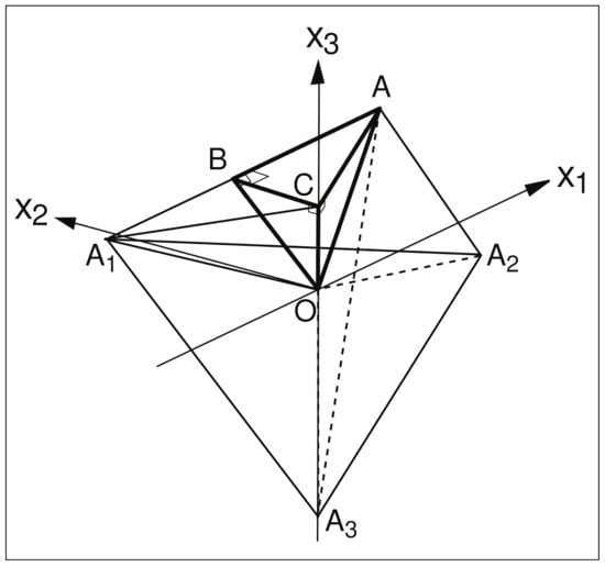
Figure 1.
Barycentric eigenvalue space. In the principal tetrahedron , for ordered eigenvalues, O represents a perfect depolarizer; A represents a deterministic system; B represents a system with two equal nonzero eigenvalues; and C represents a system with three equal nonzero eigenvalues. Each of the triangular faces of is a right-angled triangle. For unordered eigenvalues, the regular tetrahedron contains all physical states of depolarization, with at A, etc. The principal tetrahedron is of the volume of the regular tetrahedron.
We find that matrices operating on four-vectors are useful for transforming between different coordinate systems. The matrix together with its prefactor is orthogonal, so its inverse is equal to its transpose, as are the following transformation matrices. This system was chosen slightly differently from our previous studies (a uniform scaling and ordering) [87,92]. Then, inside the principal tetrahedron,
The net of the principal barycentric tetrahedron, showing the directions of the components of , is illustrated in Figure 2.
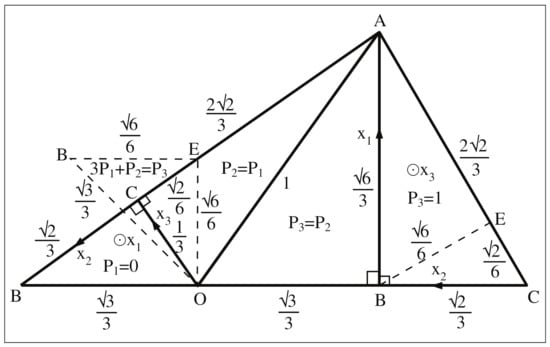
Figure 2.
The net of the principal barycentric tetrahedron for ordered eigenvalues, viewed from the outside. A perfect depolarizer is represented by point O and a pure system by point A. All the faces are right-angled triangles. Triangles ABO and BCO are similar. The basis vectors and the lengths of the edges are shown. Sixteen of these tetrahedra combine to give the regular tetradron for unordered eigenvalues and 72 to give the original cube defined by the Stokes condition. The tetrahedron corresponds to nonnegative , with on the plane .
The eigenvalues are related to the coordinates :
where is the four-vector of the eigenvalues. San José and Gil defined a purity space on their set of indices of purity, ; , [84]. Their purity space is simply the principal barycentric eigenvalue space, with our coordinates scaled independently, i.e., nonisotropically, along each axis: , , . gives the relative strength of the dominant component of the characteristic decomposition; gives the relative strength of the fully depolarized component. The indices of purity have been found to be a useful contrast mechanism in biological imaging [13]. However, the isotropic barycentric purity space has the advantages that contours of constant degree of polarimetric purity are simply spherical surfaces and also that the complete regular tetrahedron can be used to represent the variation in state with a parameter.
The eigenvalues of an Hermitian matrix are purely real. They can be calculated using Viète’s method, which gives a geometric solution based on the trigonometry of multiple angles [93,94,95]. This approach has been applied to the polarization case in 3D and 4D [87,92,96,97]. The eigenvalues of the Hermitian matrix are solutions of the characteristic equation, which is a quartic in 4D and a cubic in 3D. For scattering in the exact backscattering direction, the Hermitian matrices become of Rank 3, so there are only three nonzero eigenvalues [56,98]. For the coherency matrix there are, in addition, zeros along a row and column. For this reason, and also because the coherency matrix is more simply related to the intrinsic polarization properties, we prefer the coherency matrix to the correlation matrix . For a Rank 4 coherency matrix, the characteristic equation is a quartic, which is solved by generating the resolvent cubic, which has roots , where . We find that for the canonical Type-1 Mueller matrix, we can identify that , and generalizing to 4D vectors, , with . The four-vectors , , and are not true vectors. In image processing they are called homogeneous vectors, and they project to a three-vector. On the other hand is a true four-vector. Equation (11) can be easily adjusted so that it relates to , so we now recognize that the Euclidean space spanned by introduced by Simon et al. is, with a simple isotropic scaling, the space of . So, the first step towards calculating the eigenvalues of the coherency matrix corresponding to a Type-1 canonical Muller matrix, using Viète’s method, is effectively calculating the elements of the canonical Mueller matrix.
The coordinate systems , and are rotated with respect to each other in the same 4D space. Additionally, and are rotated with respect to each other in 3D space. We then have for the degree of polarimetric purity,
Hence, we see that for a Type-I canonical Mueller matrix is equal to the Lorentz polarization index [82]. The values of the components of within the principal barycentric tetrahedron satisfy [92]
The values of on the surface of the principal tetrahedron were plotted in Reference [92], and several other parameters were plotted in Reference [87]. These surface nets can be cut out and assembled as 3D tetrahedra, to illustrate the behavior throughout the volume. is zero on the plane in Figure 2, so is nonnegative in the tetrahedron , for which , or . At point E, ; ; and . If the determinant of a Type-I canonical Mueller matrix is negative, then is negative. The region of negative seems to be associated with anomalous depolarization, which is known to be unlikely to occur but has been shown theoretically to be possible for Mie backscattering from spherical particles [76,88,90]. The region corresponds (Equation (6)), or [87]. Although this region was first identified using entropy, other measures of depolarization can also make it visible, so entropy itself is not fundamentally related to anomalous depolarization [88,90].
The eigenvalues of the coherency matrix are given by the symmetric (and orthogonal) matrix [87,92]:
The coordinate is given by
The degree of polarimetric purity written as a four-vector is
where , so . Note that the matrix in Equation (18) is not orthogonal, because of the nonisotropic nature of . The coordinates are, however, mutually perpendicular, so the matrix in (18) is an homogeneous matrix. If they are extended over the regular tetrahedron, the points have coordinates , , , and .
Three-dimensional barycentric eigenvalue space can be regarded as being a subspace, a projection, of a 4D space spanned by the four-vector . The coordinates , in the 3D barycentric space are orthogonal and isotropic, but the alternative coordinate system is not isotropic.
A system with a Type-1 canonical Mueller matrix is represented by a point in this barycentric space and is equivalent to a corresponding Mueller matrix with elements , where , and to a diagonal matrix with elements . In our previous studies, we plotted the variation of different depolarization measures over the surface of the barycentric tetrahedron [87,92]. These plots were intended to allow mental visualization of the variations over 3D principal barycentric space, rather than suggesting that the values on the surface planes of the tetrahedron should be regarded as other than special cases, as seemed to be interpreted by Ossikovski and Vizet [90].
3.3. Type-II Canonical Mueller Matrices
Similarly, the other types of canonical Mueller matrix can be also represented by points in the same barycentric space, although the relationship with the elements of and are different. Type-II canonical Mueller matrices are Rank 2 or 3 and therefore reside in the / triangle , with , . We have for the Mueller matrix in Equation (9), ,
The eigenvalues of are . The eigenvalues of are . Then
Note that these are different for a Type-II canonical Mueller matrix. This is not surprising as the Mueller matrix retains some diattenuation. They become equal in the limiting case as , when the Type-II matrix becomes Type-I. Other parameters could prove useful, as we discuss below: for example, Gil’s degree of spherical purity eliminates the contribution of the diattenuation and polarizance [85],
For the form of Type-II canonical matrix described by Ossikovski [82], for which , this reduces to .
We find that
Figure 3 shows the state of depolarization in barycentric eigenvalue space as functions of the parameters and . If the eigenvalues are taken as ordered, the state is on or within the triangle . Then, and . However, an advantage of the barycentric space over the space of purity indices is that the trajectory as the parameters are varied can include unordered eigenvalues on or within the equilateral triangle . This approach was applied to the case of exact backscattering with rotational symmetry in a previous study [92]. The expressions for the eigenvalues of are valid even if is negative. Cases outside of the triangle correspond to different orderings of the eigenvalues, so they can be considered as being reflected into the triangle , as was described by Ossikovki and Vizet [90]. This process is reminiscent of the Brillouin zone approach, as compared to the extended zone scheme, in solid-state physics. For completeness, Simon et al’s Type-III is Rank 1, at point A; and Type-IV is Rank 2, at point B [80].
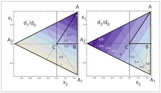
Figure 3.
The state of depolarization in barycentric eigenvalue space for the coherency matrix associated with a Type-II canonical Mueller matrix as functions of the parameters and . If the eigenvalues are taken as ordered, the state is on or within the triangle . For unordered eigenvalues, the state is on or within the equilateral triangle .
3.4. An Example
As an example of a diagonalizable Mueller matrix, we consider the case of a high-temperature phase of a polycrystalline cholesteric liquid crystal reported by Flack et al. and discussed by Ossikovski [82,99]. The Mueller matrix is
The original matrix gives and . These are different from each other, signifying the presence of diattenuation. The diagonal, Type-I canonical matrix gives and . These are equal, as there is no diattenuation. The value of is also unaltered, within numerical accuracy, as diagonalization is a similarity transformation of . This can be compared with an orthogonal (rotational) transformation of the coherency matrix, to make the off-diagonal elements purely imaginary and the off-diagonal part of the Mueller matrix skew-symmetric [100]. This operation was proposed for 3D polarization coherency matrices but is equally valid for 4D coherency matrices. Then, we obtained and ; so, again, these are almost equal as there is no diattenuation and equal to the original , as the operation constitutes a similarity transformation on .
This comparison suggests alternative measures of purity. In Gil’s expression for the degree of polarimetric purity in terms of the components of purity, [85,101]. Diattenuation results in a symmetric Mueller matrix, so putting , then the parameter , where
takes account of the diattenuation of the Mueller matrix. We call the diattenuation-corrected purity. For our example, . This value is close to , illustrating that there is depolarization for some input polarizations, and it has the desirable properties that it can be calculated without diagonalizing the Mueller matrix or calculating eigenvalues. For the rotated coherency matrix (and similarly for the diagonal matrix), , and so within numerical error. For a Type-II canonical Mueller matrix, , as in Equation (9), we also have .
3.5. Summary
Although Ossikovski and Vizet call their space a “natural depolarization space”, their eigenvalues are normalized by the largest eigenvalue, [90]. This has the effect of changing the relative significance of the eigenvalues. It is as though they are treating as an homogeneous vector rather than a true four-vector. It is therefore perhaps more natural to normalize by the sum of the eigenvalues, equal to . Then, the four eigenstates, represented by each of the eigenvalues being unity, can be plotted in 3D barycentric space, which in our view is more natural: it is an isotropic projection of 4D space onto 3D space. Then, constant values of the degree of purity are given by spherical surfaces in barycentric space. It is a Euclidean vector space, with Euclidean norms and distances. The coordinates are not naturally orthogonal in 3D space. Another advantage of barycentric space is that it is also represented by the coordinates , which are intricately connected with the geometrical model for the eigenvalue evaluation [87]. These coordinates can be calculated directly from the third-order reduced characteristic polynomial of the coherency matrix . The ’s can be plotted directly over the regular tetrahedron [92]. On the other hand, the coordinates are defined relative to the principal tetrahedron for ordered eigenvalues. This last property is also true for the coordinates , so that we have for the points , , , and , where these coordinates can take negative values for this extended domain. It is interesting to consider that as the cubic reduced characteristic equation gives the squares of the ’s, it may be related to the matrix representation described by Cloude [50].
Ossikovski and Vizet’s “natural depolarization space” is the 3D analogue of a 2D plot of the eigenvalues of the polarization coherency matrix for 3D polarized light presented by Petrucelli et al. [102]. Another way to present the data, also for 3D polarization, was proposed by Qian and Eberley [103]. They recognized that as the eigenvalues are nonnegative, then we can plot against the square roots of the eigenvalues as coordinates, in which case a constant value of lies on the surface of a sphere. However, this approach is not so useful for the 4D case, as we need to consider a hyperspherical surface in a 4D space with coordinates and the square roots of the eigenvalues. We have mentioned before that an analogy with the case of 3D polarization can lead to interesting results for the 4D case [38,100], and we anticipate future results [104,105].
Ossikovski has recognized the advantage of expressing the state of depolarization in terms of the square roots of the eigenvalues of , which gives information about the intrinsic depolarization properties, rather than [82]. The barycentric space of the coherency matrix associated with the canonical Mueller matrix is also a useful approach for representing the intrinsic depolarization state and exhibits the same advantages we have described for the extrinsic depolarization properties as compared with Ossikovski and Vizet’s canonical depolarization space [90]. The eigenvalues of are invariant when performing the symmetric decomposition, but a different set is obtained for the eigenvalues of . For the most usual practical case of a Type-I canonical Mueller matrix, as there is no diattenuation, constant values of the Lorentz degree of polarimetric purity are then represented by spherical surfaces in canonical barycentric eigenvalue space. The barycentric plot of the coherency matrix eigenvalues can be plotted over the complete regular tetrahedron for unordered eigenvalues. For ordered eigenvalues it is plotted over the irregular principal tetrahedron . For a Type-II canonical Mueller matrix, is zero, and the state is represented as a point on the plane , its distance from O being given by , in this case being unrelated to the barycentric eigenvalue plot. Two parameters (e.g., and ) are necessary to specify the state of depolarization. The combination of original and canonical indices of purity thus provide more information about the state of depolarization.
4. Discussion: Reflectance Imaging with a Beam Splitter
4.1. Polarization in Transmittance and Reflectance
It is interesting that the development of polarization theory occurred independently in optics and in polarimetric radar. In radar, the backward scattering alignment (BSA) is often used [26,28,36,55,71,78], which makes many of the equations different from those in the optical case. In optical imaging, a reflectance geometry is often used, so knowledge of the radar work is relevant. In a recent study, we examined polarization in reflectance geometry, using the Mueller matrix, the coherency matrix, and the coherency vector, [98]. For a deterministic system, the coherency matrix is [106,107,108]. We compared the Jones matrix with the Sinclair matrix, and we compared the Mueller, Mueller–Sinclair, and Kennaugh matrices. We examined the effect of various mathematical operations on the Mueller matrix and its transpose and the corresponding effects on the Jones matrix and coherency vector, extending the work of Hovenier [67]. Here we discuss the effects of utilizing a beam splitter in an optical system. Note that radar systems, using transmitter and receiver antennas, are different in this respect.
The coherency matrix has a special form for exact backscattering. It has zeros along the row and column for , the index j running , and is at most of Rank 3 [29,59,60]. This results in the Mueller matrix having a particular symmetry and the Kennaugh matrix becoming a symmetric matrix. This is only strictly true for exact backscattering from single scattering events, when light scattered from different particles can interfere coherently. Van de Hulst considers the case of approximate backscattering, where some symmetry properties are evident [29]. Optical systems with low numerical aperture can satisfy the exact backscattering condition in the limiting case.
For reflection by a perfect mirror, the Mueller matrix is diag , which we denote , the suffices denoting the negative elements. The Mueller–Sinclair matrix for reflection by a perfect mirror is the identity matrix, . So, the Sinclair form effectively “undoes” the change caused by reflection, so that other features of the resulting Mueller matrix specify polarization effects present in addition to the reflection process. In our study, we went on to consider a polarizing layer situated on a perfect reflector, with light being reflected back through the layer [98]. We proposed modeling reflectance from a medium as an effective medium on a perfect reflector, and, more specifically, as a uniform (sometimes called homogeneous) medium on a perfect reflector. This model is different from the case of direct backscattering from a nonisotropic medium [86].
The polarization transformation represented by a deterministic Mueller matrix can be represented by a Jones matrix , where
and the elements of the coherency vector are the elements of the Jones matrix written in the Pauli basis. The coherency vector for perfect reflection is , where the minus sign accounts for the phase change on reflection, giving for the Mueller matrix the diagonal matrix, .
We take the Sinclair matrix (the Sinclair form of the Jones matrix) as [98]
where are the elements of the Jones matrix. Other works define it differently, omitting the first negative sign or the complex conjugation [71]. The Sinclair form of the Mueller matrix (the Mueller–Sinclair matrix) is . The Kennaugh matrix can be formed from the Mueller matrix by changing the sign of the penultimate row [71]. Then . The Mueller matrix for light traveling in the reverse direction through a reciprocal medium is [33]. In the corresponding coherency vector, the sign of is altered, but the other elements are unchanged ([98], Table 1, line 11). The Mueller–Sinclair and Kennaugh matrices are , and . For the Sinclair system the sign of is altered with respect to ([98], Table 1, line 12). For travel through a reciprocal medium, with Mueller matrix , and then perfect reflection back through the medium in the exact backscattering direction, the total Mueller and Mueller–Sinclair matrices are , and [33], and the Kennaugh matrix is [78], as the Kennaugh matrix for exact backscattering through a reciprocal medium is symmetric ().
4.2. Backscattering through a Reciprocal Medium
The coherency vector and Sinclair coherency vector after exact backscattering through a reciprocal medium are [98]
where the elements after backscattering are denoted by single primes. For a medium with Mueller matrix , for exact backscattering , so , and for a deterministic medium, , is symmetric, and . So, has zeros along the penultimate row and column and is of Rank 3. The Sinclair coherency vector for exact backscattering with reciprocity has a zero last element, and the corresponding coherency matrix has zeros along the last row and column.
The trace conditions for single scattering in the exact backscattering direction are, for , , and , , , and , respectively [60,78,98].
Optical systems based on reflectance geometry usually incorporate a beam splitter. We consider two alternative arrangements, the first with reflection by the beam splitter after light has traveled through and back through the sample and the second where the reflection by the beam splitter occurs before the sample. For reflection by the beam splitter after the sample (denoted by double prime), . From our table of operations on the Mueller matrix ([98], Table 1, line 17), for a deterministic medium,
Comparing with Equation (27), we see that the coherency vector is just the complex conjugate of the Sinclair coherency vector with no beam splitter.
For reflection by the beam splitter before the sample (denoted by triple prime), . From our table of operations on the Mueller matrix ([98], Table 1, lines 5 or 18), for a deterministic medium,
So using a beam splitter in either position has a similar effect to calculation of the Mueller–Sinclair matrix. In particular, the zero in the coherency vector is moved from the penultimate element to the last element.
We thus obtained for these two cases using a beam splitter, in analogy with Equation (27),
For a mirror with no medium, the coherency vector with a beam splitter, in both cases, was , and the Mueller matrix is the identity matrix. So, the reflection from the mirror was canceled with the effect of the beam splitter.
For the general case, we can establish from Equation (30) the relationships, analogous to those in our previous study [98],
where R is a constant. For a uniform medium, must be purely real, where is the amplitude absorption parameter for a single transmission through the uniform medium, thus determining the absolute phases of . The global phase change of a polarization transformation represents the geometric phase for a path on the Poincaré sphere, which is unmeasurable using a conventional polarimeter. For any medium, not necessarily a uniform one, the original and final states are fixed by the values of the elements , and so it can be considered to behave as an equivalent uniform medium, for which R is real.
4.3. Some Special Cases
There are only three independent equations in Equation (31), and four unknowns, so in general there is not enough information to solve the inverse problem. However, if we know the medium has no circular diattenuation or retardence, i.e., , we find that
For the case of reflection by the beam splitter before, rather than after, the sample, then , the remaining elements of the coherency vector being unchanged. For the special cases of either a pure linear diattenuator or a pure linear retarder, are purely real, so and are also purely real, and the measured coherency vector elements correctly predict directly the orientation of the diattenuation or retardance. These can therefore be used to calibrate the optical system [2]. However, such a simple relationship does not hold for general linear diattenuation and retardance because of the phase of in Equation (32). If there are no circular diattenuation or birefringence, then the sample’s coherency vector is
where is the diattenuation; is the retardance; and and are the orientations of the diattenuation and birefringence, respectively. Then, , which should be distinguished from , and the parameters D, , , and can be determined from the components of the coherency vector. The retardance and diattenuation apply for a single pass through the sample, whereas the measured signal is for a reflection back through the sample.
For a medium aligned with the horizontal axis, for which ,
For a medium aligned with the ±45 directions, for which ,
For a weakly polarizing medium, e.g., in the limit of an optically thin layer (so that second-order terms can be neglected), , and we have the first order of small quantities, , . In this case, cannot be determined as any just changes the value of that is predicted by the measured R, by using Equation (31). In general for a medium with no linear diattenuation or retardance, for which , then , and , and and cannot be separately determined.
The trace conditions for exact backscattering with reflection by a beam splitter, for reflection after or before the sample become and , respectively, i.e., in both cases the condition is the same as for the Mueller–Sinclair matrix for a system without a beam splitter.
4.4. Some Numerical Examples
We continue by examining some experimental Mueller matrices published in the literature. The first is a birefringent tape, used as a sample in a reflectance polarization imaging system [3]. The Mueller matrix, after correction for the microscope optics, and the corresponding coherency matrix were
The elements of are given to two decimal places here, but more places were kept in the subsequent manipulations. The trace sum was , which is close to zero. The eigenvalues of the coherency matrix were , , , and to three decimal places. The negative eigenvalues must result from experimental error and were set to zero, giving a depolarization index P of 0.93.
The normalized Mueller matrix for the dominant pure component was
and the corresponding coherency vector is . However, there is a small nonzero component, which is recognized as experimental error. We chose to set the elements of the last row and column of to zero, to give a valid Mueller matrix for a reflectance system with a beam splitter, which then gives a renormalized Mueller matrix
The depolarization index was then 0.96, greater than for the original Mueller matrix with the negative eigenvalues set to zero. The renormalized Mueller matrix of the dominant pure component was
Note that these last two Mueller matrices automatically satisfy the trace condition for a reflectance system with a beam splitter and also exhibit the correct symmetry properties, , . The corresponding coherency vector is . If we assume that there is no circular birefringence or diattenuation, we can use Equation (32) to obtain the coherency vector of the sample . We obtained , and . The diattenuation was weak. The retardance and birefringence orientation (for a single pass) agreed quite well with those determined by Lu–Chipman decomposition [3].
The second example we considered was a linear polarizer (LP ColorPol VISIR, Codixx, contrast > 100,000:1), which is also used as a sample in a reflectance polarization imaging system [2]. The value of for an ideal polarizer is . The Mueller matrix, after correction for the microscope optics, and the corresponding coherency matrix were
We see that all the elements of the penultimate and last rows and columns are weak. The trace sum was , which is close to zero. The eigenvalues of the coherency matrix were , , , and to three decimal places, all non-negative to two decimal places. Setting the negative eigenvalue to zero, the calculated depolarization index P was .
The normalized Mueller matrix for the dominant deterministic component was
and the corresponding coherency vector was . Again there was a nonzero component, and we chose to set the elements of the last row and column of to zero. This gives a renormalized Mueller matrix
The depolarization index P was again found to be equal to 0.86. The renormalized Mueller matrix of the dominant pure component was
The corresponding coherency vector was .
If we assume that there is no circular birefringence or diattenuation, we can use Equation (32) to obtain the coherency vector of the sample, . We obtained , and . The diattenuation was close to aligned along the axis. The result for was not very accurate, as it was calculated as a ratio of two small quantities.
5. Conclusions
Depolarization has been found to be a useful contrast mechanism in imaging [4,13,88]. A full description of depolarization requires three parameters, so the degree of polarimetric purity , or the depolarization power, , while giving averaged measures of depolarization, do not give full details. Several different combinations of measures, constituting a 3D depolarization space, have been proposed. In addition to [38,48], the entropy S [50]; the higher-order degrees of purity , , and [87,90]; and the overall purity index [88] are functions of the eigenvalues of the coherency matrix. Other measure that give rise to depolarization spaces are the indices of purity [84] and the components of purity [85]. Other purity spaces include the “natural” depolarization space [90] and the barycentric eigenvalues space [87]. Some of the parameters are not independent variables for the almost ideally depolarized or almost pure cases. For example, for nearly deterministic systems, and [87]. For systems approximating an ideal depolarizer, [87]. For systems with two approximately equal largest eigenvalues, and [87]. The “natural” depolarization space is not an isotropic projection from 4D eigenvalue space; the space based on the indices of purity is nonisotropically scaled. In both these cases, surfaces of constant value of the degree of polarimetric purity are not spherical. Barycentric eigenvalue space avoids these problems. It is a Euclidean vector space, ideally suitable for fitting to experimental data or finding a physical or deterministic approximation. On the other hand, if used to specify brightness or color in an image display, the parameters are scaled to fill the dynamic range, and so the coordinates or are equally suitable.
Three-dimensional barycentric eigenvalue space can be regarded as being spanned by coordinates that can be represented by the four-vectors: , , and . These coordinates are isotropic, but the alternative coordinate is not isotropic, as it is nonuniformly scaled. A system with a Type-I canonical Mueller matrix is represented by a point in this barycentric space and is equivalent to a corresponding Mueller matrix with elements , where . Similarly, the other types of canonical Mueller matrix are also represented by points in the barycentric space. Type-II resides in triangle , Type-III at point A, and Type-IV at point B.
Ossikovski showed that measures based on the eigenvalues of the coherency matrix still do not tell the whole story concerning depolarization and introduced the Lorentz depolarization indices [82]. In order to account for the diattenuation of the Mueller matrix, a depolarization measure called the diattenuation-corrected purity, , was introduced in the present study. Specification of the depolarization condition using coherency matrix eigenvalues for both an original Mueller matrix and its canonical form was also proposed.
A reflectance polarization imaging system using a beam splitter, in the exact backscattering direction, gives a coherency vector with a zero in the final element, and a coherency matrix, which is at most Rank 3, with zeros in the last row and column. The Mueller matrix can be decomposed into a sum of up to three deterministic components. The Mueller matrix is similar to the Sinclair–Mueller matrix for exact backscattering without a beam splitter. For a sample placed in the optical system on a mirror, the polarimetric properties of the sample can be recovered in some cases, if we have some prior information.
Funding
This research received no external funding.
Institutional Review Board Statement
Not applicable.
Informed Consent Statement
Not applicable.
Conflicts of Interest
The authors declare no conflict of interest.
Symbols
The following symbols are used in this manuscript (some symbols have multiple meanings):
| Eigenvalue product polarimetric purity | |
| Vector form of the coherency matrix | |
| Coherency matrix | |
| Diattenuation vector | |
| d | Diattenuation |
| Orthogonal coordinate system for purity space | |
| Minkowski metric | |
| Correlation matrix | |
| Stokes parameters | |
| Jones matrix | |
| Sinclair matrix | |
| Kennaugh matrix | |
| First and second Lorentz depolarization indices | |
| Mueller matrix elements | |
| Mueller matrix | |
| Mueller spherical sub-matrix | |
| Diattenuator Mueller matrix | |
| Retarder Mueller matrix | |
| Mueller matrix for a perfect reflector | |
| Mueller-Sinclair matrix | |
| Type-I, II canonical Mueller matrix | |
| Polarization (coherency) matrix | |
| Vector form of the polarization (coherency) matrix | |
| Polarizance vector | |
| p | Polarizance |
| Degree of spherical purity | |
| Degree of polarimetric purity | |
| Second Lorentz degree of polarimetric purity | |
| Indices of purity | |
| Overall purity index | |
| Parke matrix | |
| Third order polarimetric purity | |
| Stokes vector | |
| Stokes vector in Chandrasekhar phase basis | |
| S | Entropy |
| Fourth order polarimetric purity | |
| Singular values | |
| Trace | |
| Orthogonal coordinate system for purity space | |
| Coherency vector | |
| Polarization coupling matrix, Z-matrix, or state generating matrix | |
| Depolarization power | |
| Identity matrix with elements in subscript negative | |
| transformation matrix, | |
| Transformation matrix of elements of the Pauli spin matrices | |
| Vector of eigenvalues of the coherency matrix | |
| Eigenvalues of the coherency matrix |
References
- Clivas, X.; Marquis-Weible, F.; Salathé, R.P.; Novak, R.P.; Gilgen, H.H. High-resolution reflectometry in biological tissues. Opt. Lett. 1992, 17, 4–6. [Google Scholar] [CrossRef]
- Le Gratiet, A.; Rivet, S.; Dunbreuil, M.; Le Grand, Y. 100 khz Mueller polarimeter in reflection configuration. Opt. Lett. 2015, 40, 645–648. [Google Scholar] [CrossRef] [PubMed]
- Le Gratiet, A.; d’Amora, M.; Duocastello, M.; Marongiu, R.; Bendandi, A.; Giordani, S.; Bianchini, P.; Diaspro, A. Zebra fish structural development in Mueller-matrix scanning microscopy. Sci. Rep. 2019, 9, 19974. [Google Scholar] [CrossRef] [PubMed]
- Le Gratiet, A.; Bendandi, A.; Sheppard, C.J.R.; Diaspro, A. Polarimetric optical scanning microscopy of zebrafish embryonic development using the coherency matrix. J. Biophoton. 2021, 14, e202000494. [Google Scholar] [CrossRef] [PubMed]
- Bueno, J.M.; Campbell, M.C.W. Confocal scanning laser ophthalmoscopy improvement by use of Mueller-matrix polarimetry. Opt. Lett. 2002, 27, 830–832. [Google Scholar] [CrossRef] [PubMed]
- Lara, D.; Dainty, J.C. Axially resolved complete Mueller matrix confocal microscopy. Appl. Opt. 2006, 45, 1917–1930. [Google Scholar] [CrossRef]
- Davidson, M.; Kaufman, K.; Mazor, I.; Cohen, F. An application of interference microscopy to integrated circuit inspection and metrology. Proc. SPIE 1987, 775, 233–247. [Google Scholar]
- Hee, M.R.; Huang, D.; Swanson, E.A.; Fujimoto, J.G. Polarization-sensitive low-coherence reflectometer for birefringence characterization and ranging. J. Opt Soc. Am. B 1992, 9, 903–908. [Google Scholar] [CrossRef]
- De Boer, J.F.; Milner, T.E.; van Gemert, M.J.C.; Nelson, J.S. Two-dimensional birefringence imaging in biological tissue by polarization-sensitive optical coherence tomography. Opt. Lett. 1997, 22, 934–936. [Google Scholar] [CrossRef]
- Jiao, S.; Wang, L. Two-dimensional depth-resolved Mueller matrix of biological tissue measured with double-beam polarization-sensitive optical coherence tomography. Opt. Lett. 2002, 27, 101–103. [Google Scholar] [CrossRef]
- Götzinger, E.; Pircher, M.; Geitzenauer, W.; Ahlers, C.; Baumann, B.; Michels, S.; Schmidt-Erfurth, U.; Hitzenberger, C.K. Retinal pigment epithelium segmentation by polarization sensitive optical coherence tomography. Opt. Express 2008, 16, 16410–16422. [Google Scholar] [CrossRef]
- Ortega-Quijano, N.; Marvdashti, T.; Ellerbee, A.K. Enhanced depolarization contrast in polarization- sensitive optical coherence tomography. Opt. Lett. 2016, 41, 2350–2353. [Google Scholar] [CrossRef]
- Van Eeckout, A.; Lizana, A.; Garcia-Caurel, E.; Gil, J.J.; Ossikovski, R.; Campos, J. Synthesis and characterization of depolarizing samples based on the indices of polarimetric purity. Opt. Lett. 2017, 42, 4155–4158. [Google Scholar] [CrossRef]
- Sheppard, C.J.R.; Wilson, T. Multiple traversing of the object in the scanning microscope. Opt. Acta 1980, 27, 611–624. [Google Scholar] [CrossRef]
- Ode, T. Study on confocal transmission. In Proceedings of the 9th Meeting Japan Society for Laser Microscopy, Kyoto, Japan, 1–5 June 1992; pp. 4–7. [Google Scholar]
- Stokes, G.G. On the composition and resolution of streams of polarized light from different sources. Trans. Camb. Philos. Soc. 1852, 9, 399–416. [Google Scholar]
- Verdet, E. Leçons d’Optique Physique; Imprimeri Impériale: Paris, France, 1869. [Google Scholar]
- Poincaré, H. Théorie Mathématique de la Lumière; Jacques Gabay: Paris, France, 1892. [Google Scholar]
- Soleillet, F. Sur les paramètres caractérisant la polarisation partielle de la lumière dans les phénomènes de fluorescence. Ann. Phys. 1929, 12, 23–59. [Google Scholar] [CrossRef]
- Jones, R.C. A new calculus for the treatment of optical systems. I. Description and discussions of the calculus. J. Opt. Soc. Am. 1941, 31, 488–493. [Google Scholar] [CrossRef]
- Perrin, F. Theory of light scattering by macroscopically isotropic bodies. J. Chem. Phys. 1942, 10, 415–427. [Google Scholar] [CrossRef]
- Jones, R.C. A new calculus for the treatment of optical systems. V. A more general formulation, and description of another calculus. J. Opt. Soc. Am. 1947, 37, 107–110. [Google Scholar] [CrossRef]
- Chandrasekhar, S. On the radiative equilibrium of a stellar atmos- phere: XVII. Astrophys. J. 1947, 105, 441–460. [Google Scholar] [CrossRef]
- Parke, N.G., III. Matrix Optics. Ph.D. Thesis, MIT, Cambridge, MA, USA, 1948. [Google Scholar]
- Jones, R.C. A new calculus for the treatment of optical systems. VII. Properties of the N-matrices. J. Opt. Soc. Am. 1948, 38, 671–685. [Google Scholar] [CrossRef]
- Sinclair, G. The transmision and reception of elipticaly polarized waves. Proc. IRE 1950, 38, 148–151. [Google Scholar] [CrossRef]
- Falkoff, D.L.; MacDonald, J.E. On the Stokes parameters for polarized radiation. J. Opt. Soc. Am. 1951, 41, 861–862. [Google Scholar] [CrossRef]
- Kennaugh, E. Polarization Properties of Radar Reflections. Master’s Thesis, Ohio State University, Columbus, OH, USA, 1950. [Google Scholar]
- Van de Hulst, H. Light Scattering by Small Particles; Wiley: New York, NY, USA, 1957. [Google Scholar]
- Barakat, R. Theory of the coherency matrix for light of arbitrary spectral bandwidth. J. Opt. Soc. Am. 1963, 53, 317–323. [Google Scholar] [CrossRef]
- O’Neil, E.L. Introduction to Statistical Optics; Addison-Wesley: Reading, MA, USA, 1963. [Google Scholar]
- Marathay, A.S. Operator formalism in the theory of partial polarization. J. Opt. Soc. Am. 1965, 55, 969–980. [Google Scholar] [CrossRef]
- Sekera, Z. Scattering matrices and reciprocity relationships for various representations of the state of polarization. J. Opt. Soc. Am. 1966, 56, 1732–1740. [Google Scholar] [CrossRef]
- Go, N. Optical activity of anisotropic solutions: II. J. Phys. Soc. Jpn. 1967, 23, 88–97. [Google Scholar] [CrossRef]
- Schmieder, R.W. Stokes-algebra formalism. J. Opt. Soc. Am. 1969, 59, 297–302. [Google Scholar] [CrossRef]
- Huynen, J.R. Phenomological Theory of Radar Targets; Drukkerij Bronder-Offset N.V.: Rotterdam, The Netherlands, 1970. [Google Scholar]
- Whitney, C. Pauli-algebraic operators in polarization optics. J. Opt. Soc. Am. 1971, 61, 1207–1213. [Google Scholar] [CrossRef]
- Samson, J.C. Descriptions of the polarization states of vector processes: Applications to ULF magnetic fields. Geophys. J. R. Astron. Soc. 1973, 34, 403–419. [Google Scholar] [CrossRef]
- Robson, B.A. The Theory of Polarization Phenomena; Clarendon Press: Oxford, UK, 1974. [Google Scholar]
- Jensen, H.P.; Schellman, J.A.; Troxell, T. Modulation techniques in polarization spectroscopy. Appl. Spectrosc. 1978, 32, 192–200. [Google Scholar] [CrossRef]
- Schellman, J.A.; Jensen, H.P. Optical spectroscopy of oriented molecules. Chem. Rev. 1987, 87, 1359–1399. [Google Scholar] [CrossRef]
- Schönhofer, A.; Kuball, H.-G.; Puebla, C. Optical activity of oriented molecules. IX. Phenomenological Mueller matrix description of thick samples and of optical elements. Chem. Phys. 1983, 76, 453–467. [Google Scholar] [CrossRef]
- Schönhofer, A.; Kuball, H.-G. Symmetrery properties of the Mueller matrix. Chem. Phys. 1987, 115, 159–167. [Google Scholar] [CrossRef]
- Barakat, R. Bilinear constraints between elements of the 4×4 Mueller-Jones transfer matrix of polarization theory. Opt. Commun. Am. 1981, 38, 159–161. [Google Scholar] [CrossRef]
- Fry, E.S.; Kattawar, G.W. Relationships between elements of the Stokes matrix. Appl. Opt. 1981, 20, 2811–2814. [Google Scholar] [CrossRef]
- Simon, R. The connection between Mueller and Jones matrices of polarization optics. Opt. Commun. 1982, 42, 293–297. [Google Scholar] [CrossRef]
- Gil, P.P.; Bernabeu, E. A depolarization criterion in Mueller matrices. Opt. Acta 1985, 32, 259–261. [Google Scholar] [CrossRef]
- Gil, P.P.; Bernabeu, E. Depolarization and polarization indices of an optical system. Opt. Acta 1986, 33, 185–189. [Google Scholar] [CrossRef]
- Gil, P.P.; Bernabeu, E. Obtainment of the polarizing and retardation parameters of a non-depolarizing optical system from the polar decomposition of its Mueller matrix. Optik 1987, 76, 67–71. [Google Scholar]
- Cloude, S.R. Group theory and polarization algebra. Optik 1986, 75, 26–36. [Google Scholar]
- Kim, K.; Mandel, L.; Wolf, E. Relationship between Jones and Mueller matrices for random media. J. Opt. Soc. Am. A 1987, 4, 433–437. [Google Scholar] [CrossRef]
- Barakat, R. Conditions for the physical realizability of polarization matrices characterizing passive systems. J. Mod. Opt. 1987, 34, 1535–1544. [Google Scholar] [CrossRef]
- Simon, R. Mueller matrices and depolarization criteria. J. Mod. Opt. 1987, 34, 569–575. [Google Scholar] [CrossRef]
- Chipman, R.A. Polarization Aberrations. Ph.D. Thesis, University of Arizona, Tucson, AZ, USA, 1987. [Google Scholar]
- Holm, W.; Barnes, R. On radiation polarization mixed target state decomposition techniques. In Proceedings of the 1988 Radar Conference, Ann Arbor, MI, USA, 20–21 April 1988; pp. 249–254. [Google Scholar]
- Cloude, S.R. Conditions for the physical realisability of matrix operators in polarimetry. Proc. SPIE 1989, 116, 177–185. [Google Scholar]
- Simon, R. Nondepolarizing systems and degree of polarization. Opt. Commun. 1990, 77, 349–354. [Google Scholar] [CrossRef]
- Silverman, M.P.; Badoz, J. Light reflection from a naturally optically active birefringent medium. J. Opt. Soc. Am. A 1990, 7, 1163–1173. [Google Scholar] [CrossRef]
- Mishchenko, M.I. Enhanced backscattering of polarized light from discrete random media: In exactly the backscattering direction. J. Opt. Soc. Am. A 1992, 9, 978–982. [Google Scholar] [CrossRef]
- Mishchenko, M.I.; Hovenier, J.W. Depolarization of light backscattered by randomly oriented nonspherical particles. Opt. Lett. 1995, 20, 1356–1358. [Google Scholar] [CrossRef]
- Sanjay Kumar, M.; Simon, R. Characterization of Mueller matrices in polarization optics. Opt. Commun. 1992, 88, 464–470. [Google Scholar] [CrossRef]
- Xing, Z.-F. On the deterministic and non-deterministic Mueller matrix. J. Mod. Opt. 1992, 39, 461–484. [Google Scholar] [CrossRef]
- Givens, C.R.; Kostinski, A.B. A simple necessary and sufficient condition on physically realizable Mueller matrices. J. Mod. Opt. 1993, 40, 471–481. [Google Scholar] [CrossRef]
- Van der Mee, C.V.M. An eigenvalue criterion for matrices transforming Stokes parameters. J. Math. Phys. 1993, 34, 5072–5088. [Google Scholar] [CrossRef]
- Anderson, D.G.M.; Barakat, R. Necessary and sufficient conditions for a Mueller matrix to be derivable from a Jones matrix. J. Opt. Soc. Am. A 1994, 11, 2305–2319. [Google Scholar] [CrossRef]
- Sridar, R.; Simon, R. Normal form for Mueller matrices in polarization optics. J. Mod. Opt. 1994, 41, 1903–1915. [Google Scholar] [CrossRef]
- Hovenier, J.W. Structure of a general pure Mueller matrix. Appl. Opt. 1994, 33, 8318–8324. [Google Scholar] [CrossRef]
- Hovenier, J.W.; Van der Mee, C.V.M. Testing scattering matrices; A compendium of recipes. J. Quant. Spectrosc. Radiat. Transf. 1996, 55, 649–661. [Google Scholar] [CrossRef]
- Lu, S.-Y.; Chipman, R.A. Interpretation of Mueller matrices based on polar decomposition. J. Opt. Soc. Am. A 1996, 13, 1106–1113. [Google Scholar] [CrossRef]
- Cloude, S.R.; Pottier, E. A review of target decomposition theorems in radar polarimetry. IEEE Trans. Geosci. Remote Sens. 1996, 34, 498–518. [Google Scholar] [CrossRef]
- Lüneburg, E.; Cloude, S.R. Radar versus optical polarimetry. Proc. SPIE 1997, 3120, 361–372. [Google Scholar]
- Bolshakov, Y.; van der Mee, C.V.M.; Ran, A.C.M.; Reichstein, B.; Rodman, L. Polar decompositions in finite dimensional indefinite scalar product spaces: Special cases and applications. Oper. Theory Adv. Appl. 1996, 87, 61–94, Erratum in Integr. Equ. Oper. Theory 1997, 27, 497–501. [Google Scholar] [CrossRef]
- Rao, A.V.G.; Mallesh, K.S.; Sudha. On the algebraic characterization of a Mueller matrix in polarization optics, I. Identifying a Mueller matrix from its N matrix. J. Mod. Opt. 1998, 45, 955–987. [Google Scholar] [CrossRef]
- Rao, A.V.G.; Mallesh, K.S.; Sudha. On the algebraic characterization of a Mueller matrix in polarization optics, II. Necessary and sufficient conditions for Jones-derived Mueller matrices. J. Mod. Opt. 1998, 45, 989–999. [Google Scholar]
- Gil, J.J. Characteristic properties of Mueller matrices. J. Opt. Soc. Am. 2000, 17, 328–334. [Google Scholar] [CrossRef]
- Aiello, A.; Woerdman, J.P. Physical bounds to the entropy-depolarization relation in random light scattering. Phys. Rev. Lett. 2005, 94, 090406. [Google Scholar] [CrossRef]
- Cloude, S.R. Depolarization by aerosols: Entropy of the Amsterdam light scattering database. J. Quant. Spectrosc. Radiat. Transf. 2009, 110, 1665–1676. [Google Scholar] [CrossRef]
- Cloude, S.R. Polarization: Applications in Remote Sensing; Oxford University Press: Oxford, UK, 2009. [Google Scholar]
- Ossikovski, R. Analysis of depolarizing Mueller matrices through a symmetric decomposition. J. Opt. Soc. Am. A 2009, 26, 1109–1118. [Google Scholar] [CrossRef]
- Simon, B.N.; Simon, S.; Mukunda, N.; Gori, F.; Santarsiero, M.; Borghi, R.; Simon, R. A complete characterization of pre- Mueller and Mueller matrices in polarization optics. J. Opt. Soc. Am. A 2010, 27, 188–199. [Google Scholar] [CrossRef]
- Ossikovski, R. Canonical forms of depolarizing Mueller matrices. J. Opt. Soc. Am. A 2010, 27, 123–130. [Google Scholar] [CrossRef]
- Ossikovski, R. Alternative depolarization criteria for Mueller matrices. J. Opt. Soc. Am. A 2010, 27, 808–814. [Google Scholar] [CrossRef]
- Ossikovski, R. Differential matrix formalism for depolarizing anisotropic media. Opt. Lett. 2011, 36, 2330–2332. [Google Scholar] [CrossRef]
- San José, I.; Gil, J.J. Invariant indices of polarimetric purity. Generalized indices of purity for n × n covariance matrices. Opt. Commun. 2011, 284, 38–47. [Google Scholar] [CrossRef]
- Gil, P.P. Components of purity of a Mueller matrix. J. Opt. Soc. Am. A 2011, 28, 1578–1585. [Google Scholar] [CrossRef] [PubMed]
- Arteaga, O.; Garcia-Caurel, E.; Ossikovski, R. Elementary polarization properties in the backscattering configuration. Opt. Lett. 2014, 39, 6050–6053. [Google Scholar] [CrossRef] [PubMed]
- Sheppard, C.J.R. Geometry of the Mueller matrix spectral decomposition. J. Opt. Soc. Am. A 2016, 33, 1331–1340. [Google Scholar] [CrossRef]
- Tariq, A.; Li, P.; Chen, D.; Lv, D.; Ma, H. Physically realizable space for the purity-depolarization plane for polarized light scattering media. Phys. Rev. Lett. 2017, 119, 033202. [Google Scholar] [CrossRef] [PubMed]
- Kuntman, E.; Kuntman, M.A.; Arteaga, O. Vector and matrix states for Mueller matrices of nondepolarizing optical media. J. Opt. Soc. Am. A 2017, 34, 80–86. [Google Scholar] [CrossRef]
- Ossikovski, R.; Vizet, J. Eigenvalue-based depolarization metric spaces for Mueller matrices. J. Opt. Soc. Am. A 2019, 36, 1173–1186. [Google Scholar] [CrossRef]
- Sheppard, C.J.R.; Bendandi, A.; Le Gratiet, A.; Diaspro, A. Eigenvalues of the coherency matrix for exact backscattering. J. Opt. Soc. Am. A 2019, 36, 1540–1550. [Google Scholar] [CrossRef]
- Sheppard, C.J.R.; Bendandi, A.; Le Gratiet, A.; Diaspro, A. Eigenvectors of polarization coherency matrices. J. Opt. Soc. Am. A 2020, 37, 1143–1154. [Google Scholar] [CrossRef]
- Nickalls, R.W.D. The quartic equation: Invariants and Euler’s solution revealed. Math. Gaz. 2009, 93, 66–75. [Google Scholar] [CrossRef]
- Nickalls, R.W.D. The quartic equation: Alignment with an equivalent tetrahedron. Math. Gaz. 2012, 96, 49–55. [Google Scholar] [CrossRef][Green Version]
- Nickalls, R.W.D. A new approach to solving the cubic: Cardan’s solution revealed. Math. Gaz. 1993, 77, 354–359. [Google Scholar] [CrossRef]
- Sheppard, C.J.R. Partial polarization in three dimensions. J. Opt. Soc. Am. A 2011, 28, 2655–2659. [Google Scholar] [CrossRef]
- Sheppard, C.J.R. Geometric representation for partial polarization in three dimensions. Opt. Lett. 2012, 37, 2772–2774. [Google Scholar] [CrossRef] [PubMed]
- Sheppard, C.J.R.; Bendandi, A.; Le Gratiet, A.; Diaspro, A. Polarization in reflectance imaging. J. Opt. Soc. Am. A 2020, 37, 491–500. [Google Scholar] [CrossRef] [PubMed]
- Flack, J.H.; Crooker, P.P.; Svoboda, R.C. Measurement of the Mueller matrices of blue-phase structures. Phys. Rev. A 1982, 26, 723–726. [Google Scholar] [CrossRef]
- Dennis, M. Geometric interpretation of the three-dimensional coherence matrix for nonparaxial polarization. J. Opt. A Pure Appl. Opt. 1982, 6, S26–S31. [Google Scholar] [CrossRef]
- Sheppard, C.J.R. Parameterization of the Mueller matrix. J. Opt. Soc. Am. A 2016, 33, 2323–2332. [Google Scholar] [CrossRef]
- Petrucelli, J.C.; Moore, N.J.; Alonso, M.A. Two methods for modeling the propagation of the coherence and polarization properties of nonparaxial fields. Opt. Commun. 2010, 283, 4457–4466. [Google Scholar] [CrossRef]
- Qian, X.F.; Eberley, J.H. Entanglement and classical polarization states. Opt. Lett. 2011, 36, 4110–4112. [Google Scholar] [CrossRef] [PubMed]
- Gil, J.J. Geometric interpretation and general classification of three-dimensional polarization states through the intrinsic Stokes parameters. Photonics 2021, 8, 315. [Google Scholar] [CrossRef]
- Sheppard, C.J.R.; Bendandi, A.; Le Gratiet, A.; Diaspro, A. Purity of three-dimensional polarization. J. Opt. Soc. Am. A 2022, 39, 6–16. [Google Scholar] [CrossRef]
- Sheppard, C.J.R.; Castello, M.; Diaspro, A. Expressions for parallel decomposition of the Mueller matrix. J. Opt. Soc. Am. A 2016, 33, 741–751. [Google Scholar] [CrossRef] [PubMed]
- Sheppard, C.J.R.; Le Gratiet, A.; Diaspro, A. Factorization of the coherency matrix of polarization optics. J. Opt. Soc. Am. A 2018, 35, 586–590. [Google Scholar] [CrossRef]
- Sheppard, C.J.R.; Bendandi, A.; Le Gratiet, A.; Diaspro, A. Coherency and differential Mueller matrices for polarizing media. J. Opt. Soc. Am. A 2018, 35, 2058–2069. [Google Scholar] [CrossRef]


Publisher’s Note: MDPI stays neutral with regard to jurisdictional claims in published maps and institutional affiliations. |
© 2022 by the authors. Licensee MDPI, Basel, Switzerland. This article is an open access article distributed under the terms and conditions of the Creative Commons Attribution (CC BY) license (https://creativecommons.org/licenses/by/4.0/).