Blind Restoration of Images Distorted by Atmospheric Turbulence Based on Deep Transfer Learning

 ,
,
Abstract
:1. Introduction
- (1)
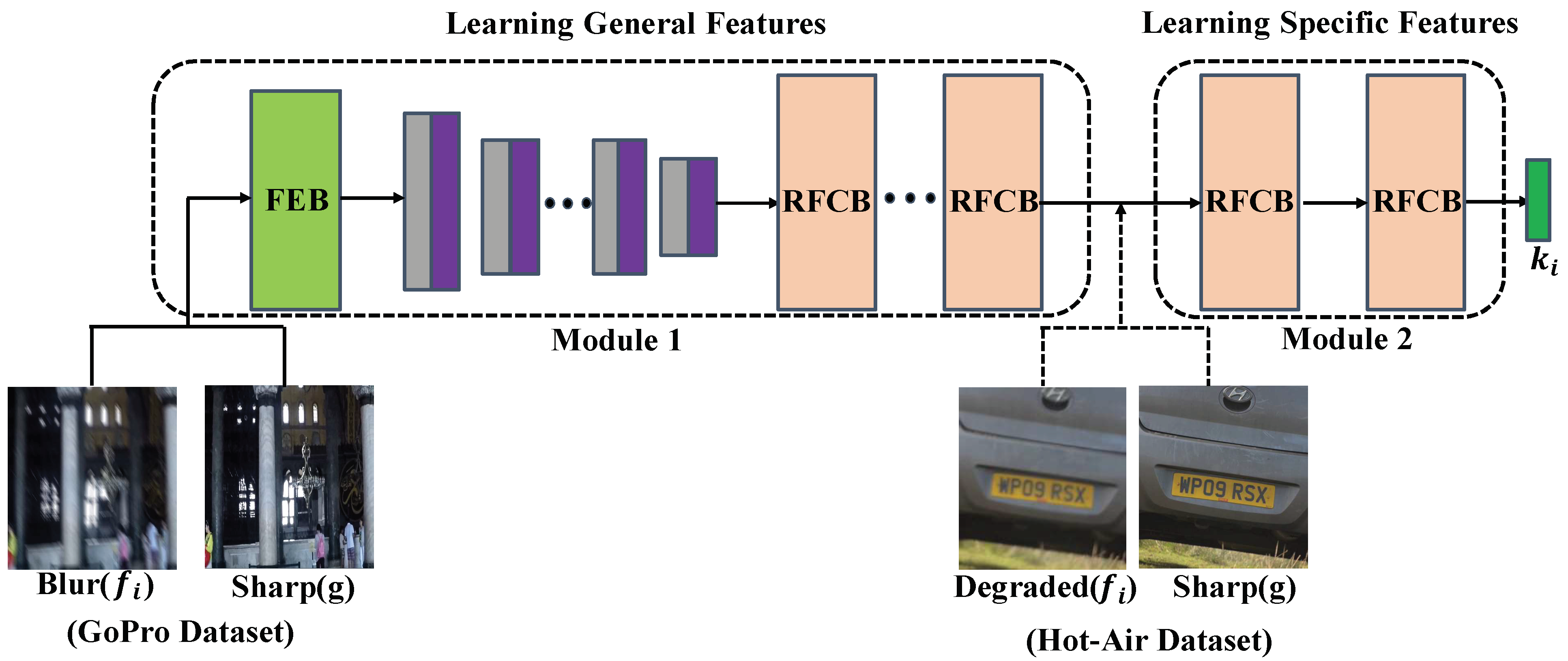
- We propose a new deep transfer learning (DTL) framework to remove the turbulence effect from real-world data. Considering that the real degraded image contains non-uniform blur, geometric deformation, and no large of paired data, we trained the proposed network by using the GoPro Dataset and a small amount of the Hot-Air Dataset, respectively.
- (2)
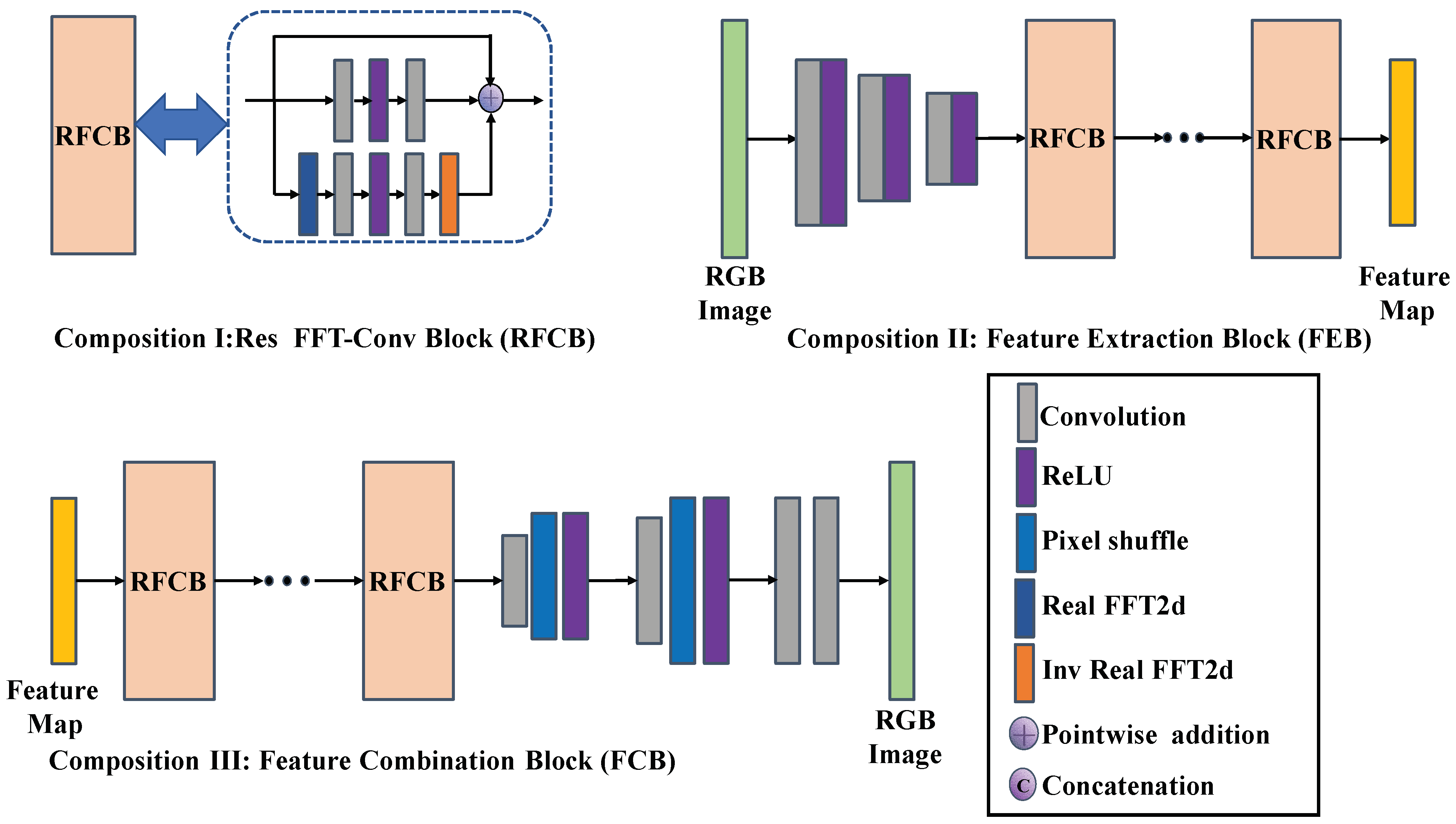
- As the conventional residual block tends to overlook the low-frequency information when reconstructing a sharp image, Res FFT-Conv Block was introduced so that the proposed framework integrated both low-frequency and high-frequency components.
- (3)
- We conducted extensive experiments by incorporating the proposed approach, and the experimental results show the performance when removing geometric distortions and blur effects can be significantly improved.
2. Related Work
3. Proposed Method
3.1. Training Dataset
3.2. Transfer Learning
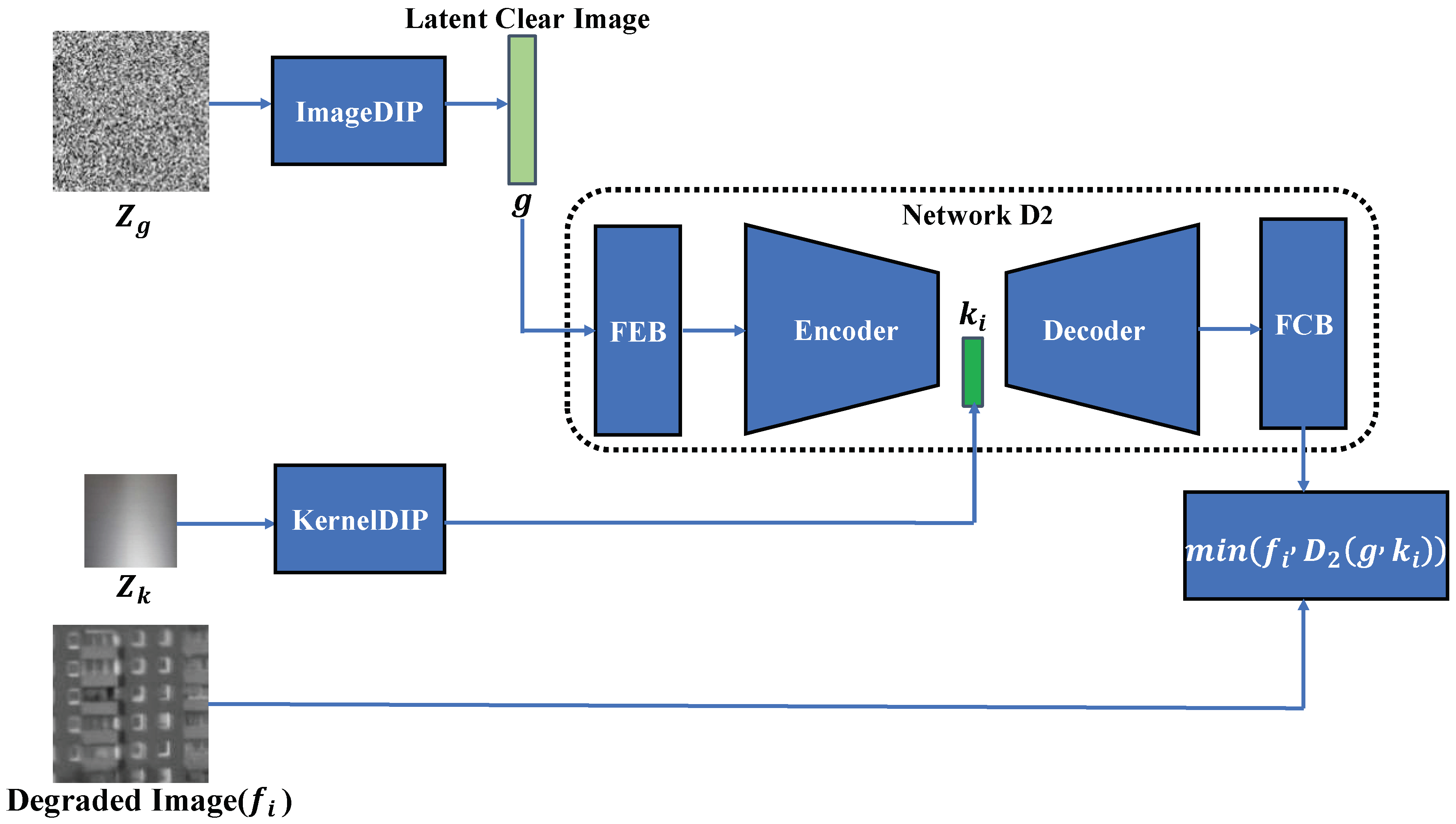
3.3. DIP Framework
3.4. Proposed Network Framework
- Step 1: Building image processing blocks
- Step 2: Training Network D
- Network D1
- Network D2

3.5. Implementation and Training Details
4. Comparative Experiment Setup
4.1. Existing Restoration Methods
4.2. Experimental Datasets
4.3. Image Quality Metrics
5. Results and Discussion
5.1. Results on the Near-Ground Turbulence Degraded Image
5.2. Results on Turbulence Degraded Astronomical Object
5.3. Results on Our Dataset
5.4. Ablation Study
6. Conclusions
Author Contributions
Funding
Institutional Review Board Statement
Informed Consent Statement
Data Availability Statement
Acknowledgments
Conflicts of Interest
References
- Maor, O.; Yitzhaky, Y. Continuous tracking of moving objects in long-distance imaging through a turbulent medium using a 3D point cloud analysis. OSA Contin. 2020, 3, 2372–2386. [Google Scholar] [CrossRef]
- Roggemann, M.C.; Welsh, B.M.; Hunt, B.R. Imaging through Turbulence; CRC Press: Boca Raton, FL, USA, 1996. [Google Scholar]
- Kopeika, N.S. A System Engineering Approach to Imaging; SPIE Press: Bellingham, WA, USA, 1998; Volume 38. [Google Scholar]
- Hufnagel, R.; Stanley, N. Modulation transfer function associated with image transmission through turbulent media. JOSA 1964, 54, 52–61. [Google Scholar] [CrossRef]
- Xue, B.; Liu, Y.; Cui, L.; Bai, X.; Cao, X.; Zhou, F. Video stabilization in atmosphere turbulent conditions based on the Laplacian-Riesz pyramid. Opt. Express 2016, 24, 28092–28103. [Google Scholar] [CrossRef] [PubMed]
- Lau, C.P.; Lai, Y.H.; Lui, L.M. Variational models for joint subsampling and reconstruction of turbulence-degraded images. J. Sci. Comput. 2019, 78, 1488–1525. [Google Scholar] [CrossRef]
- Zhu, X.; Milanfar, P. Removing atmospheric turbulence via space-invariant deconvolution. IEEE Trans. Pattern Anal. Mach. Intell. 2012, 35, 157–170. [Google Scholar] [CrossRef]
- Gao, Z.; Shen, C.; Xie, C. Stacked convolutional auto-encoders for single space target image blind deconvolution. Neurocomputing 2018, 313, 295–305. [Google Scholar] [CrossRef]
- Gao, J.; Anantrasirichai, N.; Bull, D. Atmospheric turbulence removal using convolutional neural network. arXiv 2019, arXiv:1912.11350. [Google Scholar]
- Zhu, P.; Xie, C.; Gao, Z. Multi-frame blind restoration for image of space target with frc and branch-attention. IEEE Access 2020, 8, 183813–183825. [Google Scholar] [CrossRef]
- Kotera, J.; Šroubek, F.; Milanfar, P. Blind deconvolution using alternating maximum a posteriori estimation with heavy-tailed priors. In Proceedings of the International Conference on Computer Analysis of Images and Patterns, York, UK, 27–29 August 2013; pp. 59–66. [Google Scholar]
- Levin, A.; Weiss, Y.; Durand, F.; Freeman, W.T. Efficient marginal likelihood optimization in blind deconvolution. In Proceedings of the CVPR 2011, Colorado Springs, CO, USA, 20–25 June 2011; pp. 2657–2664. [Google Scholar]
- Liu, H.; Zhang, T.; Yan, L.; Fang, H.; Chang, Y. A MAP-based algorithm for spectroscopic semi-blind deconvolution. Analyst 2012, 137, 3862–3873. [Google Scholar] [CrossRef]
- Wipf, D.; Zhang, H. Revisiting Bayesian blind deconvolution. J. Mach. Learn. Res. 2014, 15, 3775–3814. [Google Scholar]
- Nair, N.G.; Mei, K.; Patel, V.M. A comparison of different atmospheric turbulence simulation methods for image restoration. arXiv 2022, arXiv:2204.08974. [Google Scholar]
- Chen, G.; Gao, Z.; Wang, Q.; Luo, Q. Blind de-convolution of images degraded by atmospheric turbulence. Appl. Soft Comput. 2020, 89, 106131. [Google Scholar] [CrossRef]
- Çaliskan, T.; Arica, N. Atmospheric turbulence mitigation using optical flow. In Proceedings of the 2014 22nd International Conference on Pattern Recognition, Stockholm, Sweden, 24–28 August 2014; pp. 883–888. [Google Scholar]
- Nieuwenhuizen, R.; Dijk, J.; Schutte, K. Dynamic turbulence mitigation for long-range imaging in the presence of large moving objects. EURASIP J. Image Video Process. 2019, 2019, 2. [Google Scholar] [CrossRef] [PubMed]
- Fried, D.L. Probability of getting a lucky short-exposure image through turbulence. JOSA 1978, 68, 1651–1658. [Google Scholar] [CrossRef]
- Roggemann, M.C.; Stoudt, C.A.; Welsh, B.M. Image-spectrum signal-to-noise-ratio improvements by statistical frame selection for adaptive-optics imaging through atmospheric turbulence. Opt. Eng. 1994, 33, 3254–3264. [Google Scholar] [CrossRef]
- Vorontsov, M.A.; Carhart, G.W. Anisoplanatic imaging through turbulent media: Image recovery by local information fusion from a set of short-exposure images. JOSA A 2001, 18, 1312–1324. [Google Scholar] [CrossRef]
- John, S.; Vorontsov, M.A. Multiframe selective information fusion from robust error estimation theory. IEEE Trans. Image Process. 2005, 14, 577–584. [Google Scholar] [CrossRef]
- Li, D.; Mersereau, R.M.; Simske, S. Atmospheric turbulence-degraded image restoration using principal components analysis. IEEE Geosci. Remote Sens. Lett. 2007, 4, 340–344. [Google Scholar] [CrossRef]
- Zhu, X.; Milanfar, P. Image reconstruction from videos distorted by atmospheric turbulence. In Proceedings of the Visual Information Processing and Communication, San Jose, CA, USA, 19–21 January 2010; pp. 228–235. [Google Scholar]
- Deledalle, C.-A.; Gilles, J. BATUD: Blind Atmospheric Turbulence Deconvolution; Hal-02343041; HAL: Bengaluru, India, 2019. [Google Scholar]
- Su, C.; Wu, X.; Guo, Y.; Zhang, S.; Wang, Z.; Shi, D. Atmospheric turbulence degraded image restoration using a modified dilated convolutional network. IET Image Process. 2022. [Google Scholar] [CrossRef]
- Shi, J.; Zhang, R.; Guo, S.; Yang, Y.; Xu, R.; Niu, W.; Li, J. Space targets adaptive optics images blind restoration by convolutional neural network. Opt. Eng. 2019, 58, 093102. [Google Scholar] [CrossRef]
- Lau, C.P.; Castillo, C.D.; Chellappa, R. Atfacegan: Single face semantic aware image restoration and recognition from atmospheric turbulence. IEEE Trans. Biom. Behav. Identity Sci. 2021, 3, 240–251. [Google Scholar] [CrossRef]
- Rai, S.N.; Jawahar, C. Removing Atmospheric Turbulence via Deep Adversarial Learning. IEEE Trans. Image Process. 2022, 31, 2633–2646. [Google Scholar] [CrossRef] [PubMed]
- Hirsch, M.; Sra, S.; Schölkopf, B.; Harmeling, S. Efficient filter flow for space-variant multiframe blind deconvolution. In Proceedings of the 2010 IEEE Computer Society Conference on Computer Vision and Pattern Recognition, San Francisco, CA, USA, 13–18 June 2010; pp. 607–614. [Google Scholar]
- Anantrasirichai, N.; Achim, A.; Kingsbury, N.G.; Bull, D.R. Atmospheric turbulence mitigation using complex wavelet-based fusion. IEEE Trans. Image Process. 2013, 22, 2398–2408. [Google Scholar] [CrossRef] [PubMed]
- Nah, S.; Hyun Kim, T.; Mu Lee, K. Deep multi-scale convolutional neural network for dynamic scene deblurring. In Proceedings of the IEEE Conference on Computer Vision and Pattern Recognition, Honolulu, HI, USA, 21–26 July 2017; pp. 3883–3891. [Google Scholar]
- Keskin, O.; Jolissaint, L.; Bradley, C.; Dost, S.; Sharf, I. Hot-Air Turbulence Generator for Multiconjugate Adaptive Optics; SPIE: Bellingham, WA, USA, 2003; Volume 5162. [Google Scholar]
- Pratt, L.Y. Discriminability-based transfer between neural networks. Adv. Neural Inf. Process. Syst. 1993, 5, 204. [Google Scholar]
- Pan, S.J.; Yang, Q. A survey on transfer learning. IEEE Trans. Knowl. Data Eng. 2009, 22, 1345–1359. [Google Scholar] [CrossRef]
- Tan, C.; Sun, F.; Kong, T.; Zhang, W.; Yang, C.; Liu, C. A survey on deep transfer learning. In Proceedings of the International Conference on Artificial Neural Networks, Shenzhen, China, 8–10 December 2018; pp. 270–279. [Google Scholar]
- Wang, T.; Huan, J.; Zhu, M. Instance-based deep transfer learning. In Proceedings of the 2019 IEEE Winter Conference on Applications of Computer Vision (WACV), Waikoloa Village, HI, USA, 7–11 January 2019; pp. 367–375. [Google Scholar]
- Zhang, L.; Guo, L.; Gao, H.; Dong, D.; Fu, G.; Hong, X. Instance-based ensemble deep transfer learning network: A new intelligent degradation recognition method and its application on ball screw. Mech. Syst. Signal Process. 2020, 140, 106681. [Google Scholar] [CrossRef]
- Lin, J.; Ward, R.; Wang, Z.J. Deep transfer learning for hyperspectral image classification. In Proceedings of the 2018 IEEE 20th International Workshop on Multimedia Signal Processing (MMSP), Vancouver, BC, Canada, 29–31 August 2018; pp. 1–5. [Google Scholar]
- Song, Q.; Zheng, Y.-J.; Sheng, W.-G.; Yang, J. Tridirectional transfer learning for predicting gastric cancer morbidity. IEEE Trans. Neural Netw. Learn. Syst. 2020, 32, 561–574. [Google Scholar] [CrossRef]
- Bai, M.; Yang, X.; Liu, J.; Liu, J.; Yu, D. Convolutional neural network-based deep transfer learning for fault detection of gas turbine combustion chambers. Appl. Energy 2021, 302, 117509. [Google Scholar] [CrossRef]
- Liu, Y.; Yu, Y.; Guo, L.; Gao, H.; Tan, Y. Automatically Designing Network-based Deep Transfer Learning Architectures based on Genetic Algorithm for In-situ Tool Condition Monitoring. IEEE Trans. Ind. Electron. 2021, 69, 9483–9493. [Google Scholar] [CrossRef]
- Cheng, C.; Zhou, B.; Ma, G.; Wu, D.; Yuan, Y. Wasserstein distance based deep adversarial transfer learning for intelligent fault diagnosis. arXiv 2019, arXiv:1903.06753. [Google Scholar]
- Yu, C.; Wang, J.; Chen, Y.; Huang, M. Transfer learning with dynamic adversarial adaptation network. In Proceedings of the 2019 IEEE International Conference on Data Mining (ICDM), Beijing, China, 8–11 November 2019; pp. 778–786. [Google Scholar]
- Torrey, L.; Shavlik, J. Transfer learning. In Handbook of Research on Machine Learning Applications and Trends: Algorithms, Methods, and Techniques; IGI Global: Madison, WI, USA, 2010; pp. 242–264. [Google Scholar]
- Yosinski, J.; Clune, J.; Bengio, Y.; Lipson, H. How transferable are features in deep neural networks? arXiv 2014, arXiv:1411.1792. [Google Scholar]
- Ulyanov, D.; Vedaldi, A.; Lempitsky, V. Deep image prior. In Proceedings of the IEEE Conference on Computer Vision and Pattern Recognition, Salt Lake City, UT, USA, 18–22 June 2018; pp. 9446–9454. [Google Scholar]
- Zhu, Y.; Pan, X.; Lv, T.; Liu, Y.; Li, L. DESN: An unsupervised MR image denoising network with deep image prior. Theor. Comput. Sci. 2021, 880, 97–110. [Google Scholar] [CrossRef]
- Lai, W.-S.; Huang, J.-B.; Ahuja, N.; Yang, M.-H. Deep laplacian pyramid networks for fast and accurate super-resolution. In Proceedings of the IEEE Conference on Computer Vision and Pattern Recognition, Honolulu, HI, USA, 21–26 July 2017; pp. 624–632. [Google Scholar]
- Mao, X.; Liu, Y.; Shen, W.; Li, Q.; Wang, Y. Deep Residual Fourier Transformation for Single Image Deblurring. arXiv 2021, arXiv:2111.11745. [Google Scholar]
- Loshchilov, I.; Hutter, F. Sgdr: Stochastic gradient descent with warm restarts. arXiv 2016, arXiv:1608.03983. [Google Scholar]
- Kingma, D.P.; Ba, J. Adam: A method for stochastic optimization. arXiv 2014, arXiv:1412.6980. [Google Scholar]
- Lou, Y.; Kang, S.H.; Soatto, S.; Bertozzi, A.L. Video stabilization of atmospheric turbulence distortion. Inverse Probl. Imaging 2013, 7, 839. [Google Scholar] [CrossRef]
- Gilles, J.; Ferrante, N.B. Open turbulent image set (OTIS). Pattern Recognit. Lett. 2017, 86, 38–41. [Google Scholar] [CrossRef]
- Mittal, A.; Soundararajan, R.; Bovik, A.C. Making a “completely blind” image quality analyzer. IEEE Signal Process Lett. 2012, 20, 209–212. [Google Scholar] [CrossRef]
- Mittal, A.; Moorthy, A.K.; Bovik, A.C. No-reference image quality assessment in the spatial domain. IEEE Trans. Image Process. 2012, 21, 4695–4708. [Google Scholar] [CrossRef]
- Moorthy, A.K.; Bovik, A.C. A two-step framework for constructing blind image quality indices. IEEE Signal Process. Lett. 2010, 17, 513–516. [Google Scholar] [CrossRef]


| Categories | Approaches | Major Findings | Limitations |
|---|---|---|---|
| Physical-based approaches | Optical flow [5,17,18] | Better registration of degraded image sequence | Input multiple frames of degraded images |
| Lucky region fusion [19,20,21,22] | High quality for celestial image restoration | Lucky frame must be found | |
| Blind deconvolution [23,24,25] | Does not depend on PSF | Large amount of calculation | |
| Learning-based approaches | CNN [8,9,16,26] | Powerful feature extraction capability | Large number of paired datasets for training |
| GAN [27,28,29] | More similar to the characteristics of the real data |
| Dataset | Authors | Number | Size |
|---|---|---|---|
| GoPro Dataset | Nah et al. | 2103 pairs | 1280 × 720 |
| Hot-Air Dataset | Anantrasirichai et al. | 300 pairs | 512 × 512 |
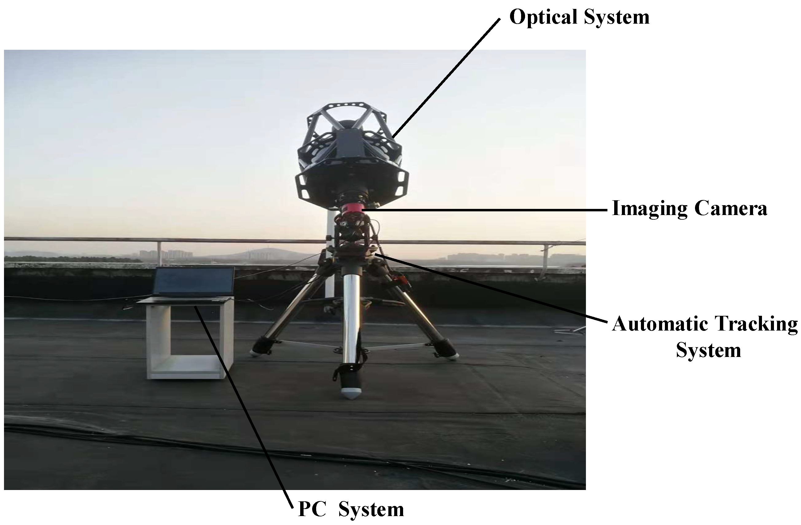
| Instrument | Hardware System Parameters |
|---|---|
| Optical System | RC 12 Telescope Tube |
| Automatic Tracking System | CELESTRON CGX-L German Equatorial Mount |
| Imaging Camera | ASI071MC Pro Frozen Camera |
| PC System | CPU: I7-9750H; RAM:16G; GPU: NVIDIA RTX 2070 |
| Entropy ↑ | NIQE ↓ | BRISQUE ↓ | BIQI ↓ | |
|---|---|---|---|---|
| Degraded Image | 6.4193 | 7.9276 | 42.8864 | 50.5454 |
| CLEAR [31] | 6.8844 | 8.6656 | 43.3481 | 54.6824 |
| SGL [53] | 6.4369 | 7.8228 | 42.8543 | 48.9341 |
| IBD [23] | 6.5116 | 11.3887 | 53.5077 | 43.5596 |
| Gao et al. [9] | 6.2806 | 9.6778 | 54.5817 | 47.6033 |
| DTL (ours) | 6.7793 | 6.0192 | 35.8791 | 35.4763 |
| Entropy ↑ | NIQE ↓ | BRISQUE ↓ | BIQI ↓ | |
|---|---|---|---|---|
| Degraded Image | 5.3926 | 12.4475 | 66.0496 | 38.4312 |
| CLEAR [31] | 5.9317 | 10.1226 | 65.9663 | 29.1219 |
| SGL [53] | 5.3501 | 11.9364 | 66.5905 | 37.0627 |
| IBD [23] | 5.3546 | 9.7114 | 64.8477 | 43.9363 |
| Gao et al. [9] | 5.6238 | 9.8788 | 54.1042 | 33.3903 |
| DTL (ours) | 5.9512 | 9.2882 | 46.0878 | 25.5453 |
| Entropy ↑ | NIQE ↓ | BRISQUE ↓ | BIQI ↓ | |
|---|---|---|---|---|
| Degraded Image | 6.7552 | 8.6912 | 37.8321 | 34.1193 |
| CLEAR [31] | 7.2909 | 7.5729 | 37.8216 | 38.0817 |
| SGL [53] | 6.7762 | 8.4834 | 37.5563 | 33.9916 |
| IBD [23] | 7.1997 | 7.6028 | 30.3502 | 28.9854 |
| Gao et al. [9] | 7.2070 | 9.9093 | 42.2126 | 33.7443 |
| DTL (Ours) | 6.9850 | 6.6927 | 18.8260 | 20.4367 |
Publisher’s Note: MDPI stays neutral with regard to jurisdictional claims in published maps and institutional affiliations. |
© 2022 by the authors. Licensee MDPI, Basel, Switzerland. This article is an open access article distributed under the terms and conditions of the Creative Commons Attribution (CC BY) license (https://creativecommons.org/licenses/by/4.0/).
Share and Cite
Guo, Y.; Wu, X.; Qing, C.; Su, C.; Yang, Q.; Wang, Z. Blind Restoration of Images Distorted by Atmospheric Turbulence Based on Deep Transfer Learning. Photonics 2022, 9, 582. https://doi.org/10.3390/photonics9080582
Guo Y, Wu X, Qing C, Su C, Yang Q, Wang Z. Blind Restoration of Images Distorted by Atmospheric Turbulence Based on Deep Transfer Learning. Photonics. 2022; 9(8):582. https://doi.org/10.3390/photonics9080582
Chicago/Turabian StyleGuo, Yiming, Xiaoqing Wu, Chun Qing, Changdong Su, Qike Yang, and Zhiyuan Wang. 2022. "Blind Restoration of Images Distorted by Atmospheric Turbulence Based on Deep Transfer Learning" Photonics 9, no. 8: 582. https://doi.org/10.3390/photonics9080582
APA StyleGuo, Y., Wu, X., Qing, C., Su, C., Yang, Q., & Wang, Z. (2022). Blind Restoration of Images Distorted by Atmospheric Turbulence Based on Deep Transfer Learning. Photonics, 9(8), 582. https://doi.org/10.3390/photonics9080582