Article

Blind Restoration of Images Distorted by Atmospheric Turbulence Based on Deep Transfer Learning

1
Key Laboratory of Atmospheric Optics, Hefei Institutes of Physical Science, Chinese Academy of Sciences, Hefei 230031, China
2
Science Island Branch of Graduate School, University of Science and Technology of China, Hefei 230026, China
3
Advanced Laser Technology Laboratory of Anhui Province, Hefei 230037, China
*
Author to whom correspondence should be addressed.
Photonics 2022, 9(8), 582; https://doi.org/10.3390/photonics9080582
Submission received: 22 July 2022 / Revised: 12 August 2022 / Accepted: 14 August 2022 / Published: 18 August 2022
(This article belongs to the Special Issue Artificial Intelligence and Machine Learning in Photonics)

Abstract

:
Removing space-time varying blur and geometric distortions simultaneously from an image is a challenging task. Recent methods (including physical-based methods or learning-based methods) commonly default the turbulence-degraded operator as a fixed convolution operator. Obviously, the assumption does not hold in practice. According to the situation that the real turbulence distorted operator has double uncertainty in space and time dimensions, this paper reports a novel deep transfer learning (DTL) network framework to address this problem. Concretely, the training process of the proposed approach contains two stages. In the first stage, the GoPro Dataset was used to pre-train the Network D1 and freeze the bottom weight parameters of the model; in the second stage, a small amount of the Hot-Air Dataset was employed for finetuning the last two layers of the network. Furthermore, residual fast Fourier transform with convolution block (Res FFT-Conv Block) was introduced to integrate both low-frequency and high-frequency residual information. Subsequently, extensive experiments were carried out with multiple real-world degraded datasets by implementing the proposed method and four existing state-of-the-art methods. In contrast, the proposed method demonstrates a significant improvement over the four reported methods in terms of alleviating the blur and distortions, as well as improving the visual quality.

1. Introduction

Atmospheric turbulence generally refers to the random fluctuation of the refractive index of the atmosphere, which significantly impacts the performance of remote imaging systems (including visual surveillance, astronomical observation, etc.) [1,2]. Specifically, this phenomenon means atmospheric turbulence that can change the path and direction of light during imaging through the random motion of the turbulent medium. When the exposure time is not short enough, the refractive index along the optical transmission path can seriously affect the image resolution, resulting in geometric distortion, defocus blur, and motion blur [3]. Essentially, this result is mainly due to the non-uniform distribution of temperature that yields random atmosphere refractive-index fluctuations, resulting in optical turbulence that distorts the wave front. Meanwhile, under the effects of the turbulent flow of air and changes in the density of air particles, humidity, and carbon dioxide levels, the refractive index also changes accordingly, which leads to space-time geometric distortion and a non-uniform blurring effect. Therefore, the real turbulence degradation process is extremely complex [4,5,6].
However, in some turbulent image restoration literature, it is considered that the point spread function (PSF) of atmospheric turbulence is time- and space-invariant. Based on this view, the degradation process of atmospheric turbulence can be regarded as a spatially linearly invariant system. As a result, the atmospheric turbulence degradation model can be expressed as follows [7,8,9,10]:
f i = H i g + n ,   or   f i = M i H i g + n ,
f i = k i g + n ,   k i = H i   or   M i H i ,
where represents convolution processing; g is the latent clear image; M i and H i are the PSFs of geometric deformation and atmospheric turbulence, respectively; n represents additive noise, which is generally represented by Gaussian noise; and f i is the ith observed image frame. Therefore, according to Equation (2), k i denotes the turbulence-degraded operator. Generally, the task of restoring a degraded image is to obtain a clear image and turbulence degraded operator based on a given observed image frame. To counter this, a popular approach to recover the sharp image is to use the Maximize A Posterior (MAP) [11,12,13,14], which is used to find g and k i to maximize the posterior probability P ( g , k i | f i ) . This expression can be seen as an optimization of the following:
g , k i = arg max g , k i P ( f i | g , k i ) P ( g ) P ( k i ) ,
In fact, this is an ill-posed problem. There are an infinite amount of pairs of ( k i , g) leading to the same probability P ( f i | g , k i ) , thus the key aspect of the above MAP approach is to define proper models for the prior distributions P(g) and P( k i ). Currently, many restoration methods focus on designing manual priors for x and k or deep learning images prior. Notably, the premise of the above-mentioned work is to assume that the turbulence degraded operator ( k i ) is a convolution operator. Obviously, these existing image processing methods use over-simplified models that are not justified and explainable by physics. As the geometric distortion and blur induced by turbulence is randomly spatially and time-varying [3], its more likely performance on degraded images is non-uniform blur and the geometric deformation effect. Therefore, these turbulence degradation models based on a fixed convolution operator are different from real-world data, and their corresponding restoration methods will have artifacts or even lose their effect on the restoration of real turbulence-degraded images. Essentially, a more accurate degradation model can be written as follows [15]:
f i = M i ( H ( g ) ) + n = k i ( g ) + n k i ( g ) ,
where H i denotes the PSF that changes over time and space, M i represents turbulence-induced deformations matrix, and their effect on the latent clear image g is embodied in the form of mapping; furthermore, k i is the fusion of H i and M i .
Another commonly used method is to directly learn a function from the turbulence degraded image to the corresponding clear image. Presently, this function is usually a deep convolutional network, and the specific parameters of the network can be obtained by training on pairs of degraded-sharp images. Moreover, different from the MAP-based method, these networks directly learn the inverse function of the turbulence degradation operator without explicitly inferring the kernel distribution of the turbulence degradation operator and the point spread function. However, such methods often rely on a large number of paired datasets for training. For the image restoration tasks in atmospheric turbulence it is difficult to obtain a massive open dataset for training and testing. Thus, these networks rely on simulated datasets in the fixed convolutional form [8,9,16], which present the same problem as the MAP-based methods.
In this article, a network framework combined with a residual block and autoencoder is presented to restore real turbulence-degraded images. Even in situations with a strong level of turbulence-induced degradation, the restoration quality is acceptable. The main contributions of this paper are as follows:
(1)
We propose a new deep transfer learning (DTL) framework to remove the turbulence effect from real-world data. Considering that the real degraded image contains non-uniform blur, geometric deformation, and no large of paired data, we trained the proposed network by using the GoPro Dataset and a small amount of the Hot-Air Dataset, respectively.
(2)
As the conventional residual block tends to overlook the low-frequency information when reconstructing a sharp image, Res FFT-Conv Block was introduced so that the proposed framework integrated both low-frequency and high-frequency components.
(3)
We conducted extensive experiments by incorporating the proposed approach, and the experimental results show the performance when removing geometric distortions and blur effects can be significantly improved.
The remainder of this paper is organized as follows. Section 2 provides a brief survey of related work. Section 3 mainly introduces the training dataset, the development and advantages of transfer learning, the overall framework of the model, and implementation details. In Section 4, four existing methods for mitigating the turbulence effect, comparative experimental datasets, and the evaluation indicators are described in detail. Section 5 presents the results and discussion. Finally, the research is concluded in Section 6.

2. Related Work

The problems regarding restoring a clear image from a sequence of turbulence-degraded frames are of high research interest. Usually, the mitigation of the effects of atmospheric turbulence is based on physical-based methods or learning-based methods. Physical-based methods mainly rely on optical flow [5,17,18], lucky region fusion [19,20,21,22], and blind deconvolution [23,24,25]. Notably, many of these methods have artifacts when reconstructing dynamic scenes with large amounts of motion. Additionally, scholars also have recently integrated neural network methodologies with the advancement of machine learning. Most of the existing networks are built based on the convolutional neural network (CNN) [8,9,16,26], as the convolution block has a powerful feature extraction capability. For example, Chen et al. employed an end-to-end deep convolutional autoencoder combined with the U-Net model to mitigate the turbulence effect [16]. Su et al. proposed a modified dilated convolutional network to restore turbulence-degraded images [26]. Subsequently, because the data generated by the Generative Adversarial Network (GAN) network have similar characteristics as the real data, more researchers have started trying to alleviate turbulence effects using GAN networks [27,28,29]. Table 1 compares the advantages and limitations of these approaches in detail.

3. Proposed Method

3.1. Training Dataset

In Section 1, the fixed convolution method used to construct the simulated training set resulted in a large difference from the natural turbulence degraded image. Air turbulence distortion is generally caused by the constantly changing refractive index field of the airflow. It typically occurs when imaging through long-range atmospheric turbulence or short-range hot air turbulence (e.g., fire flames and vapor streams). Empirically, the long-range atmospheric turbulence degraded images lack clear images as the ground truth, while short-range hot air turbulence can obtain approximate degraded-sharp image pairs by switching the gas stove on and off, but the blur effect is not significant. Therefore, this paper uses a blur dataset (GoPro Dataset) and a small amount of the Hot-Air Dataset to train the proposed model [30,31]. The GoPro Dataset was proposed by Nah et al. [32], and is a non-uniform blur dataset, which is more similar to real-world blur images. Using hot air to obtain turbulent flow effects was first proposed by [33]. Subsequently, Anantrasirichai et al. generated a number of image sequences containing objects distorted by using eight gas hobs. The flow of gas created temperature gradients that caused distortions in the scene. Thus, a certain number of clear-degraded image pairs could be obtained. The GoPro Dataset and the Hot-Air Dataset adopted by the paper are constituted as Table 2.

3.2. Transfer Learning

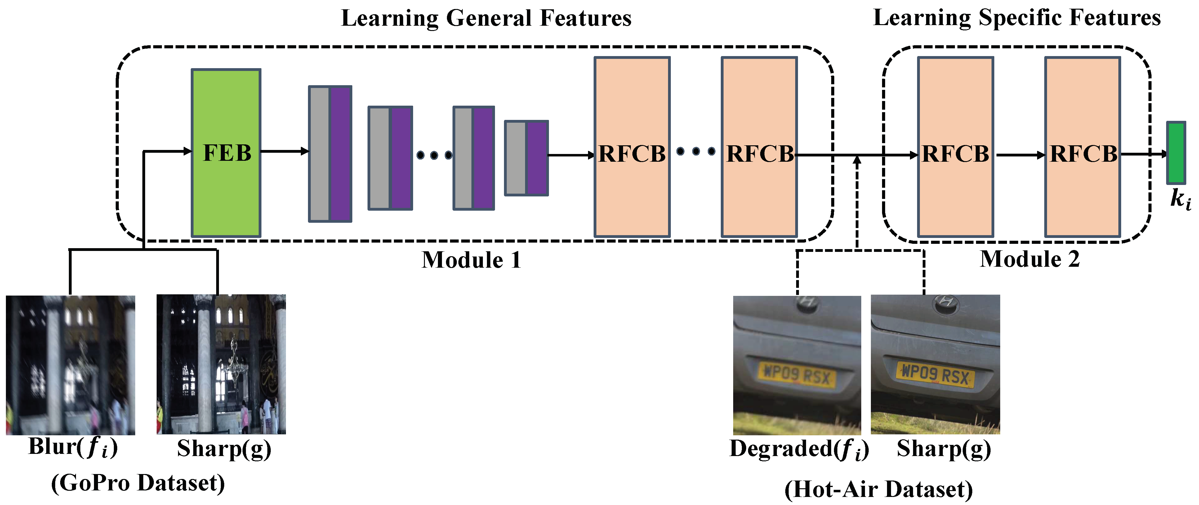
Generally, transfer learning is an important tool to solve the basic problem of insufficient training data, and it was first proposed by [34]. In 1993, Pratt et al. formulated the identifiability-based transfer (DBT) algorithm. Afterwards, Yang et al. provided a specific and comprehensive introduction to transfer learning [35]. In 2018, Tan et al. put forward the viewpoint of deep transfer learning [36], and divided deep transfer learning into (I) instance-based deep transfer learning [37,38], (II) mapping-based deep transfer learning [39,40], (III) network-based deep transfer learning [41,42], and (IV) adversarial-based deep transfer learning [43,44], which resulted in a significantly positive effect on many domains that are difficult to improve because of insufficient training data. In this research, as it was difficult to obtain massive real turbulent images with ground truth sharp references, the deep transfer learning framework was the focus of our attention. The transfer learning framework used in this paper is shown in Figure 1.
In this article, we adopted a network-based deep transfer learning framework. As shown in Figure 1, the learner learns two different tasks [45], and the fields of the two different tasks have certain similarities. Specifically, the two tasks are divided into the source domain and target domain. Generally, the source domain contains a large number of training datasets, while the target domain contains fewer available data. Our goal is to transfer the experience learned in the source domain to the target domain to help complete the specific task. According to the view put forward by [46], when deep learning is used to perform image processing, the first layers of the designed network are usually not mainly related to the specific image dataset, but the last layers of the network are closely related to the selected dataset and its mission objectives. Based on this idea, in the transfer learning framework, the first layers are generally exploited to learn general features, and the last layers are used to learn specific features. Hence, considering that the real turbulence distorted image contains both geometric deformation and space-time varying blurs, it is necessary for our model to effectively learn the two mentioned features in order to better mitigate the turbulence effects. This paper uses the GoPro Dataset [32] to pre-train the overall network to learn the non-uniform blur effect, and the Hot-Air Dataset is then employed to fine-tune the last two layers of the proposed network so as to understand geometric deformation.

3.3. DIP Framework

In 2018, Ulyanov et al. first proposed the deep image prior (DIP) framework for image restoration tasks [47], which adopts the structure of a DIP generator network to capture low-level image statistics and shows a powerful ability for image denoising, super-resolution, inpainting, etc. Subsequently, Zhu et al. proposed a combined DIP framework denoising network to obtain high-quality magnetic resonance imaging (MRI) [48]. However, there are also some drawbacks with the DIP framework. For example, the designed DIP network is limited to capturing prior blur kernels. Hence, we employed an effective network-based deep transfer learning framework to capture the turbulence-induced kernels and combined the DIP framework to alleviate the real turbulence effect.

3.4. Proposed Network Framework

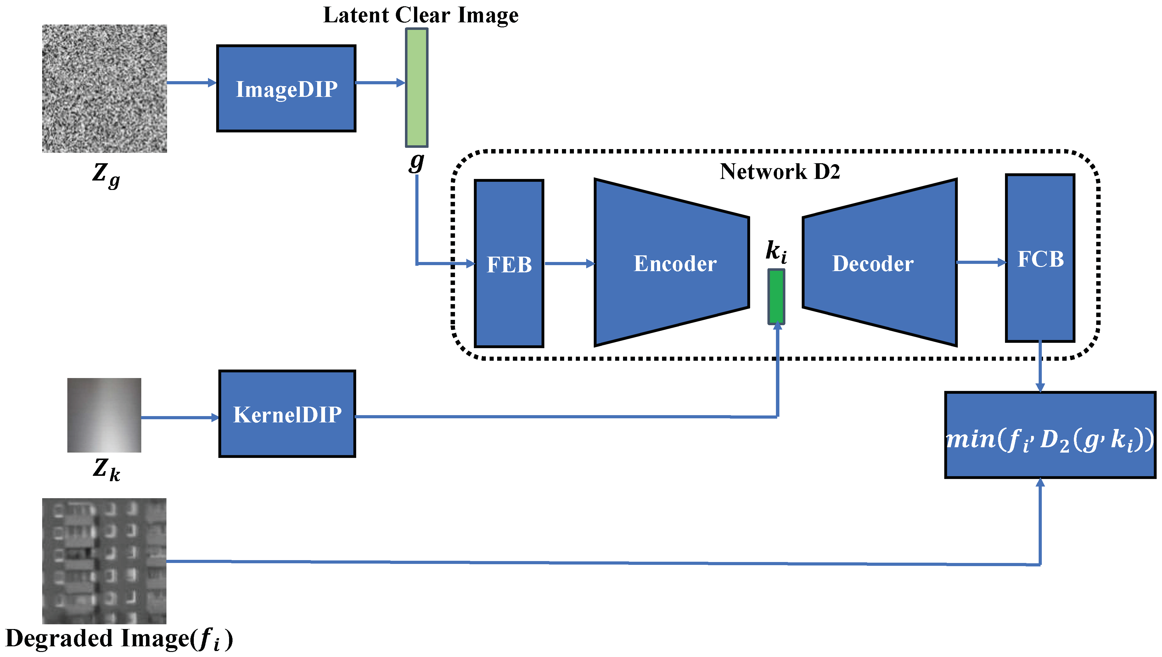
The overall structure of the inference processing is illustrated in Figure 2, which mainly includes multiple sub-networks—ImageDIP, KernelDIP, and Network D2. Concretely, (1) ImageDIP was used for generating a latent clear image, and the input Z g is a normal-distributed random tensor with size of 1 × 64 × 64. ImageDIP is mainly composed of the same encoder-decoder network with five layers. Its network composition and parameter settings are the same as in [47]. (2) The KernelDIP network was employed to output the degraded kernel k i , and its structure is equal to Network D1; the input Z k is also a normal-distributed random tensor. (3) In inference processing, Network D2 uses the latent clear image g and the turbulence degradation operator k i to reconstruct the estimated degraded image f i , and thereafter it is combined with the input degraded image ( f i ) to minimize loss [49]. The loss function can be specifically expressed as follows:
l o s s = min ( f i , D 2 ( g , k i ) ) = i = 1 n ρ ( f i , D 2 ( g , k i ) ) = i = 1 n ρ ( f i , D 2 ( I m a g e D I P ( Z x ) , K e r n e l D I P ( Z k ) ) ) ,
where ρ denotes the Charbonnier loss measuring the distance between the estimated degraded image D 2 ( ImageDIP ( Z x ) , kernelDIP ( Z k ) ) and real degraded image f i . Meanwhile, Network D2 is a part of Network D. In order to fully extract the real turbulent degradation operator, k i , we used the transfer learning framework to construct Network D. The composition and training of Network D are shown in Figure 3, Figure 4 and Figure 5.
Figure 2. The overall architecture of the proposed DTL network (inference processing).
Photonics 09 00582 g002
  • Step 1: Building image processing blocks
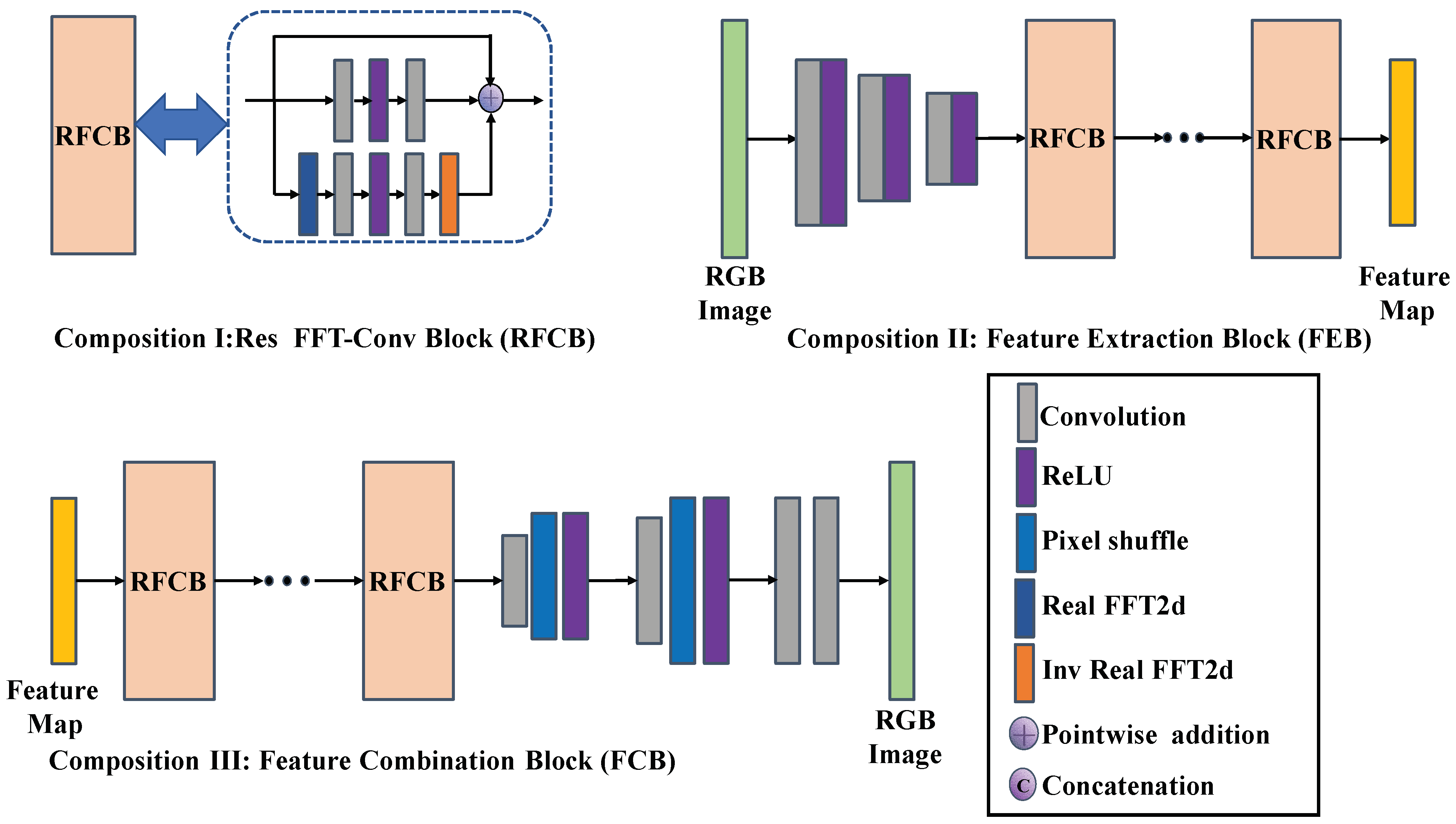
Figure 3. Structures of Res FFT-Conv Block (RFCB), feature extraction block (FEB), and feature combination block (FCB).
Photonics 09 00582 g003
In the above image processing network structure diagram, the Res FFT-Conv Block is equivalent to the composition I; this idea is inspired by the work of Mao et al. [50]. Because of the traditional residual module only capturing the high-frequency information of the image, the low-frequency features of the image could not effectively be obtained, which would have a great impact on the restoration of the real turbulence-degraded images. Therefore, the paper adopted the novel Res FFT-Conv Block to build the feature extraction block (FEB) and feature combination block (FCB). The FEB block down-sampled the input image twice and converted it to a feature map, and the FCB block converted the output feature map to the image domain. Additionally, these blocks are also important parts of Network D.
  • Step 2: Training Network D
  • Network D1
Figure 4. Block diagram of Network D1 (training processing).
Photonics 09 00582 g004
  • Network D2
Figure 5. Structure of Network D2 (training processing).
Photonics 09 00582 g005
The Step 2 modules reflect the Network D training processing. Specifically, Network D consists of Network D1 and Network D2. The turbulence degraded operator k i is extracted by the proposed deep transfer learning framework (Network D1). Furthermore, Network D1 was trained by using two datasets. First, 2103 image pairs were input to learn the non-uniformly blur as the general features of the image, then the module 1 part of the network was frozen, and a total of 300 hot-air image pairs were adopted to fine tune module 2. Notably, the Hot-Air Dataset and the GoPro Dataset were both input from the left of Network D1; as module 1 has been frozen, the actual input was equivalent to the dashed import before module 2 (see Figure 4). Moreover, Network D2 is a degraded image generator that generates the estimated f i , and k i can be continuously sent to Network D2 from Network D1. Meanwhile, in training processing, g is a sharp image from trained datasets rather than from ImageDIP. Therefore, the estimated f i can be generated by inputting g and k i . Similarly, Network D2 is trained by minimizing the Charbonnier loss of the estimated degraded image f i and the corresponding input real degraded image f i from the trained datasets.

3.5. Implementation and Training Details

We collected a total of 2403 image pairs (as shown in Table 1), and all the training images were cropped into patches with a size of 256 × 256. The proposed algorithm is was using the PyTorch1.5 deep learning framework and was trained on a single NVIDIA GTX 1080Ti GPU under the Ubuntu18.04 system. Unless specially stated, Network D2 was trained synchronously with Network D1. The training process of Network D1 is divided into two stages: (1) The GoPro Dataset is sent to the network for training, and 600,000 iterations in total are performed, so that the network can fully learn from the non-uniform blur characteristics of the image, then the weight parameters of module 1 are frozen. (2) The Hot-Air Dataset input fine-tuning module 2 parts (as shown in Figure 4), was iterated 300 times, the initial learning rate was 5 × 10⁻⁴ employing a cosine annealing scheduler [51], and Adam was used to optimize the model training [52]. Ultimately, we obtained an excellent Network D model file.

4. Comparative Experiment Setup

4.1. Existing Restoration Methods

To better analyze the performance of the proposed algorithm, we compared the proposed model with several state-of-the-art restoration methods, including three methods based on the physics model (CLEAR [31], SGL [53], and IBD [23]) and one based on the supervised learning method (Gao et al. [9]). For a fair comparison, all of the compared methods were generated using the authors’ codes, with the related parameters remaining unchanged. Meanwhile, all learning-based methods in this paper were trained on the same dataset.

4.2. Experimental Datasets

Here, the performance of our proposed network was evaluated on real degraded images using turbulence in different states. These real-world data include Hirsch’s Dataset [30], Open Turbulent Image Set (OTIS) [54], YouTube Dataset, and our dataset, respectively. These datasets are introduced as follows.
Hirsch’s Dataset: Hirsch’s Dataset was used for testing the efficient filter flow (EFF) framework. The dataset was taken using the Canon EOS 5D Mark II camera, equipped with a 200 mm zoom lens. By capturing a static scene of the hot air discharged from the vents of the building, the image sequences, which were a video stream of 100 frames (the exposure time of each frame is 1/250 s), were degraded due to spatial changes and blurring. Furthermore, the image sequences mainly included chimneys, buildings, water tanks, etc.
OTIS: OTIS was put forward by Jérôme Gilles et al. to make the comparison between algorithms. All image sequences were natural turbulence degraded images acquired in the hot summer. The dataset included 4628 static sequences and 567 dynamic sequences. The turbulence impact was also divided into three levels: strong, medium, and weak. Additionally, all sequences were captured with GoPro Hero 4 Black cameras, and the camera equipment was modified with Ribcage Air chassis in order to adapt to different lens types.
YouTube Dataset: As there is no publicly available astronomical object turbulence degradation image dataset, we downloaded some astronomical object images from YouTube. The images included several moon surface images taken by foreign astronomy enthusiasts. This part of the data capture device in particular was quite different, which added more tests for the restoration effect of the proposed algorithm.
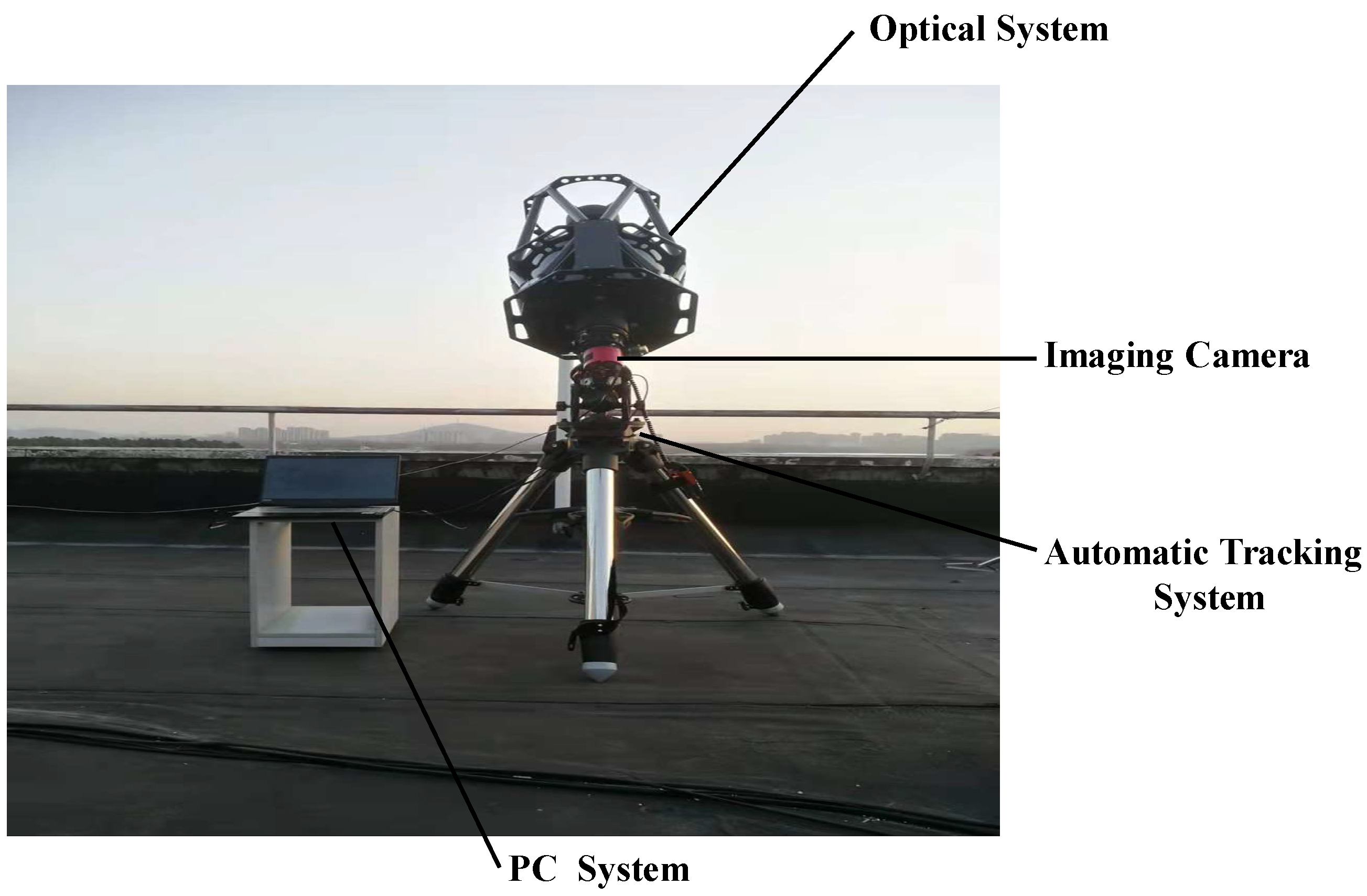
Our Dataset: We separately photographed near-ground long-distance targets and the moon with the Cassegrain-type optical telescope equipped in the laboratory. Namely, our observation system (see Figure 6), listed in Table 3, mainly included an optical system, automatic tracking system, imaging camera, and PC system.
The shooting time was selected in the afternoon and the night of 23 June 2021, and the outdoor temperature was 28–32 °C. The distance between the photographed near-ground target and the telescope was further than 5 km. Meanwhile, before the moon was observed at night, Astro Panel software was first used to monitor the cloud cover to ensure that the observing object remained unblocked as much as possible. The cloud cover monitoring diagram is shown in the left figure below (Figure 7a); the higher the blue ratio, the fewer clouds at the observation time. Therefore, the time we chose to observe the astronomical object is shown in the red box of Figure 7a, and the meteorological condition was pretty good at that time. For instance, the moon image obtained by observing at 21:00 p.m. is shown in the below right picture (Figure 7b).

4.3. Image Quality Metrics

Generally, image quality is an important measure to evaluate the perceptual and structural information present in an image. Because the comparative experiments in this article were mainly aimed at real turbulence distorted images, the performance of the proposed network and comparison methods were evaluated using multiple non-reference evaluation indexes. For instance, the indexes used included entropy, natural image quality evaluator (NIQE) [55], blind image spatial quality evaluator (BRISQUE) [56], and blind image quality indices (BIQI) [57]. Subsequently, these indicators were computed to objectively assess the quality of the restored images.

5. Results and Discussion

5.1. Results on the Near-Ground Turbulence Degraded Image

First of all, several images were selected from the OTIS [54] and Hirsch’s Dataset [30] for comparative experimental analysis. After taking into account the length of the article, four images were randomly selected for comparison of the restoration effects, and the above-mentioned no-reference indicators were used for objective evaluation. Concretely, “↑” indicates that the larger the index value, the better the image restoration effect; “↓” represents the opposite result. Thus, the test image restoration results are shown in Table 4 below.
As shown in Figure 8, the first and second rows are from OTIS, and the last rows are from Hirsch’s Dataset. It can be seen that all comparison methods and proposed approaches had a certain restoration effect on the degraded images. Through the analysis of specific indicators, whether they relied on the traditional physics model approaches or the previous supervised learning method that only depended on the training set, there were certain limitations when restoring natural turbulence-degraded images in different scenarios. Specifically, the SGL algorithm did not mitigate the turbulence effect from raw images near the ground significantly, and there was only a slight effect. This could be—because the algorithm relies on multi-frame degraded images as the input, and the information of the input single-frame turbulence degraded images was too poor. Furthermore, the CLEAR algorithm significantly improved the image information entropy and increased the image contrast, but its other indicators were terrible. Based on end-to-end, the algorithm used by Gao et al. exposed its weak generalization ability on cross-domain images, indicating that the data-driven deep learning method was less effective for data that do not meet the training requirements. In contrast, the proposed network fully considered the turbulence degraded characteristics in the natural state, learning non-uniform and geometric deformation features simultaneously; therefore, our approach finally obtained a superior performance in the test data.

5.2. Results on Turbulence Degraded Astronomical Object

The selected astronomical (the moon surface) data mainly came from image frames extracted from distorted videos downloaded from YouTube. Because these data were captured with different times, locations, and telescope system parameters, we could more thoroughly test the robustness and generalization ability of all of the mentioned methods. The specific restoration effect and index evaluation were as shown in Table 5.
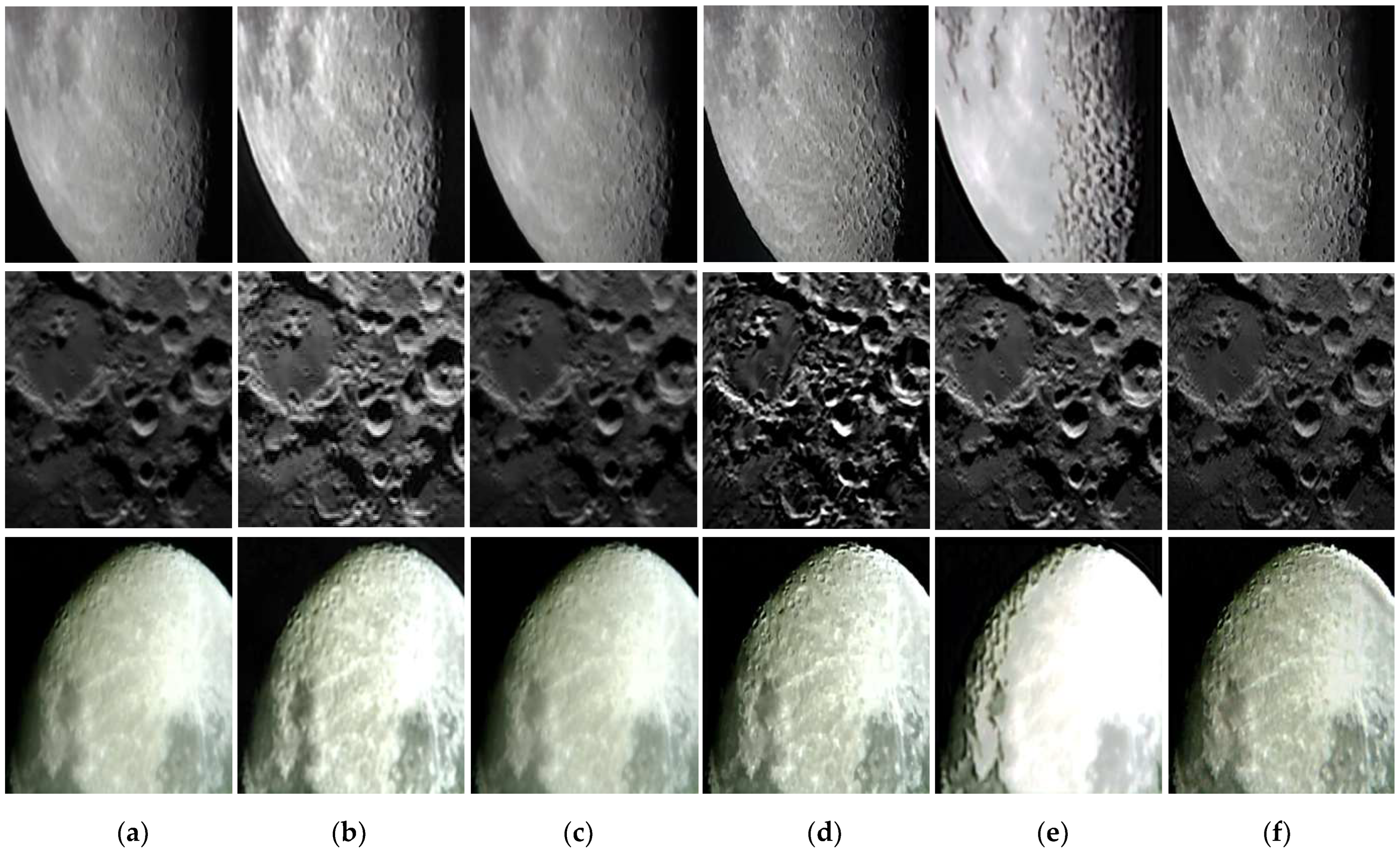
Figure 9 shows the performance of the compared algorithms and our network on the various natural astronomical images. Specifically, because the distorted images of the astronomical object contained the turbulence effect and were accompanied by multiple noises and the influence of cosmic rays, which are a great challenge for all of the mentioned restoration methods. We concluded from further analysis of the above evaluation indicators that the proposed algorithm achieved superior results for information entropy, NIQE, BRISQUE, and BIQI.

5.3. Results on Our Dataset

Considering that the number of natural turbulence corrupted images acquired only from the open dataset was still few, the atmospheric turbulence parameters of the shooting environment were not accurate enough, which would affect the subsequent atmospheric turbulence characteristic analysis. Therefore, this paper used the Cassegrain-type optical telescope system equipped in the laboratory captured the near ground (about 5–10 km away from the lens) buildings, and observed the moon image at night as the test data. The corresponding restoration results and evaluation metrics are shown in Table 6 below.
Our dataset consisted of shopping mall facades, a residential building, an iron tower, and a natural moon image. As these data were all captured in the hot summer, and the shooting distance was more than 5 km, the turbulence effect of the images was significant. From the human eye visual perception analysis, the output results of the Gao et al. network appeared distorted (see the first to third rows of Figure 10e), and this phenomenon could also be found for the indexes NIQE and BRISQUE. Moreover, the SGL algorithm and CLEAR algorithm could not thoroughly remove the turbulence effect from the test data. Not surprisingly, the proposed method still had the best performance for all comparison methods, whether the target was near the ground or the object in space.

5.4. Ablation Study

In this section, as Network D was the only part that required pre-training in the proposed DTL framework. Moreover, the estimation of the turbulence degradation operator k i was crucial for the final output. Therefore, we organized ablation experiments to test the different components of Network D1 when removing the performance of the turbulence affects. Namely, the proposed Network D1 contained two parts: a pre-trained network using the GoPro Dataset and a fine-tuned trained network on the Hot-Air Dataset, both of which could be disassembled separately to consider the degraded operator k i . Thus, the three networks for the comparison experiment were only pretrained GoPro Dataset (called D 1 _ G o Pr o ), only pretrained Hot-Air Dataset (called D 1 _ H   ot A ir ), and transfer learning framework (D1). Additionally, other parts of Network D had the same default. Thereafter, we use the mentioned no-reference evaluation indicators to evaluate different component functions of Network D1. The experiment results are shown in the following histogram.
As shown in Figure 11, three different Network D1s constituted the DTL framework, and multiple natural turbulence-degraded images were used to test the mentioned networks. The abscissa of histograms (a–d) indicated the names of the natural degraded images., the ordinate represents the no-reference evaluation index (Entropy, NIQE, BRISQUE, and BIQI), respectively. Obviously, it was found that a small amount of the Hot-Air Dataset was not enough to make the model achieve the best performance. Moreover, the GoPro Dataset only contained non-uniform blur features and no geometrical distortion features, and the trained network had a poor restoration effect on the real turbulence-distorted images. In this case, we used a few Hot-Air Dataset images to fine tune the model trained on the GoPro Dataset, and a robust and adaptable DTL framework was finally achieved. Indeed, this also verified that all components of the Network D1 were essential using the above-mentioned comparative experiments.

6. Conclusions

In this work, firstly, we propose a novel neural network framework to reconstruct a high-quality output from a single real turbulence-distorted image. Specifically, the research does not assume that the real distorted image was caused by a convolution operator (uniform blur and uniform geometric distortion); instead, it uses the implicit map to represent the turbulence degradation operator, which is more consistent with the characteristics of real turbulence-degraded images. Based on this view, the GoPro Dataset was used to learn non-uniform blur as the general features; then, freezing the network parameters, the last two layers of the network were fine-tuned by taking a limited number of images from the Hot-Air Dataset. Therefore, the proposed network can fully extract the degradation operator of real turbulence from a small amount of natural turbulence data, which has great significance for building the image restoration model in this paper.
Secondly, due to the traditional residual block that ignores the low-frequency information of the picture, a kind of plug-and-play Res FFT-Conv Block has been introduced into this framework, which can fully integrate the low-frequency and high-frequency residual information of the image.
Finally, the network proposed is fully compared with the four existing restoration methods. The objective indicators show that the proposed model has a better fusion performance and adaptability for various real turbulence-distorted images. Meanwhile, the ablation study is carried out to verify the significance of the transfer learning framework.
In the future, we plan to use a mathematical model to guide the training of our deep network to discard some unnatural artifacts and ringing effects (Figure 8f). On the other hand, more natural turbulence distorted images will be captured by our telescope system to verify the robustness and generalization ability of the network. Furthermore, we will investigate the restoration of real turbulent videos and consider embedding the model on a mobile electronic imaging platform to remove real-time turbulence.

Author Contributions

Conceptualization, Y.G. and X.W.; software, Y.G.; validation and formal analysis, Y.G. and C.Q.; data curation, Q.Y., Z.W. and C.S.; instrument, Y.G.; writing—original draft preparation, Y.G.; writing—review and editing, Y.G.; visualization, Y.G.; supervision, X.W.; project administration and funding acquisition, X.W. All authors have read and agreed to the published version of the manuscript.

Funding

This research was funded by the National Natural Science Foundation of China by Xiaoqing Wu (Grant No. 91752103), and the Foundation of Advanced Laser Technology Laboratory of Anhui Province by Chun Qing (Grant No. AHL2021QN02).

Institutional Review Board Statement

Not applicable.

Informed Consent Statement

Not applicable.

Data Availability Statement

The data were prepared and analyzed in this study.

Acknowledgments

We thank all anonymous reviewers for their comments and suggestions. In addition, the authors would like to thank Xiaoqing Wu and Chun Qing for their patience, help, and guidance.

Conflicts of Interest

The authors declare no conflict of interest.

References

  1. Maor, O.; Yitzhaky, Y. Continuous tracking of moving objects in long-distance imaging through a turbulent medium using a 3D point cloud analysis. OSA Contin. 2020, 3, 2372–2386. [Google Scholar] [CrossRef]
  2. Roggemann, M.C.; Welsh, B.M.; Hunt, B.R. Imaging through Turbulence; CRC Press: Boca Raton, FL, USA, 1996. [Google Scholar]
  3. Kopeika, N.S. A System Engineering Approach to Imaging; SPIE Press: Bellingham, WA, USA, 1998; Volume 38. [Google Scholar]
  4. Hufnagel, R.; Stanley, N. Modulation transfer function associated with image transmission through turbulent media. JOSA 1964, 54, 52–61. [Google Scholar] [CrossRef]
  5. Xue, B.; Liu, Y.; Cui, L.; Bai, X.; Cao, X.; Zhou, F. Video stabilization in atmosphere turbulent conditions based on the Laplacian-Riesz pyramid. Opt. Express 2016, 24, 28092–28103. [Google Scholar] [CrossRef] [PubMed]
  6. Lau, C.P.; Lai, Y.H.; Lui, L.M. Variational models for joint subsampling and reconstruction of turbulence-degraded images. J. Sci. Comput. 2019, 78, 1488–1525. [Google Scholar] [CrossRef]
  7. Zhu, X.; Milanfar, P. Removing atmospheric turbulence via space-invariant deconvolution. IEEE Trans. Pattern Anal. Mach. Intell. 2012, 35, 157–170. [Google Scholar] [CrossRef]
  8. Gao, Z.; Shen, C.; Xie, C. Stacked convolutional auto-encoders for single space target image blind deconvolution. Neurocomputing 2018, 313, 295–305. [Google Scholar] [CrossRef]
  9. Gao, J.; Anantrasirichai, N.; Bull, D. Atmospheric turbulence removal using convolutional neural network. arXiv 2019, arXiv:1912.11350. [Google Scholar]
  10. Zhu, P.; Xie, C.; Gao, Z. Multi-frame blind restoration for image of space target with frc and branch-attention. IEEE Access 2020, 8, 183813–183825. [Google Scholar] [CrossRef]
  11. Kotera, J.; Šroubek, F.; Milanfar, P. Blind deconvolution using alternating maximum a posteriori estimation with heavy-tailed priors. In Proceedings of the International Conference on Computer Analysis of Images and Patterns, York, UK, 27–29 August 2013; pp. 59–66. [Google Scholar]
  12. Levin, A.; Weiss, Y.; Durand, F.; Freeman, W.T. Efficient marginal likelihood optimization in blind deconvolution. In Proceedings of the CVPR 2011, Colorado Springs, CO, USA, 20–25 June 2011; pp. 2657–2664. [Google Scholar]
  13. Liu, H.; Zhang, T.; Yan, L.; Fang, H.; Chang, Y. A MAP-based algorithm for spectroscopic semi-blind deconvolution. Analyst 2012, 137, 3862–3873. [Google Scholar] [CrossRef]
  14. Wipf, D.; Zhang, H. Revisiting Bayesian blind deconvolution. J. Mach. Learn. Res. 2014, 15, 3775–3814. [Google Scholar]
  15. Nair, N.G.; Mei, K.; Patel, V.M. A comparison of different atmospheric turbulence simulation methods for image restoration. arXiv 2022, arXiv:2204.08974. [Google Scholar]
  16. Chen, G.; Gao, Z.; Wang, Q.; Luo, Q. Blind de-convolution of images degraded by atmospheric turbulence. Appl. Soft Comput. 2020, 89, 106131. [Google Scholar] [CrossRef]
  17. Çaliskan, T.; Arica, N. Atmospheric turbulence mitigation using optical flow. In Proceedings of the 2014 22nd International Conference on Pattern Recognition, Stockholm, Sweden, 24–28 August 2014; pp. 883–888. [Google Scholar]
  18. Nieuwenhuizen, R.; Dijk, J.; Schutte, K. Dynamic turbulence mitigation for long-range imaging in the presence of large moving objects. EURASIP J. Image Video Process. 2019, 2019, 2. [Google Scholar] [CrossRef] [PubMed]
  19. Fried, D.L. Probability of getting a lucky short-exposure image through turbulence. JOSA 1978, 68, 1651–1658. [Google Scholar] [CrossRef]
  20. Roggemann, M.C.; Stoudt, C.A.; Welsh, B.M. Image-spectrum signal-to-noise-ratio improvements by statistical frame selection for adaptive-optics imaging through atmospheric turbulence. Opt. Eng. 1994, 33, 3254–3264. [Google Scholar] [CrossRef]
  21. Vorontsov, M.A.; Carhart, G.W. Anisoplanatic imaging through turbulent media: Image recovery by local information fusion from a set of short-exposure images. JOSA A 2001, 18, 1312–1324. [Google Scholar] [CrossRef]
  22. John, S.; Vorontsov, M.A. Multiframe selective information fusion from robust error estimation theory. IEEE Trans. Image Process. 2005, 14, 577–584. [Google Scholar] [CrossRef]
  23. Li, D.; Mersereau, R.M.; Simske, S. Atmospheric turbulence-degraded image restoration using principal components analysis. IEEE Geosci. Remote Sens. Lett. 2007, 4, 340–344. [Google Scholar] [CrossRef]
  24. Zhu, X.; Milanfar, P. Image reconstruction from videos distorted by atmospheric turbulence. In Proceedings of the Visual Information Processing and Communication, San Jose, CA, USA, 19–21 January 2010; pp. 228–235. [Google Scholar]
  25. Deledalle, C.-A.; Gilles, J. BATUD: Blind Atmospheric Turbulence Deconvolution; Hal-02343041; HAL: Bengaluru, India, 2019. [Google Scholar]
  26. Su, C.; Wu, X.; Guo, Y.; Zhang, S.; Wang, Z.; Shi, D. Atmospheric turbulence degraded image restoration using a modified dilated convolutional network. IET Image Process. 2022. [Google Scholar] [CrossRef]
  27. Shi, J.; Zhang, R.; Guo, S.; Yang, Y.; Xu, R.; Niu, W.; Li, J. Space targets adaptive optics images blind restoration by convolutional neural network. Opt. Eng. 2019, 58, 093102. [Google Scholar] [CrossRef]
  28. Lau, C.P.; Castillo, C.D.; Chellappa, R. Atfacegan: Single face semantic aware image restoration and recognition from atmospheric turbulence. IEEE Trans. Biom. Behav. Identity Sci. 2021, 3, 240–251. [Google Scholar] [CrossRef]
  29. Rai, S.N.; Jawahar, C. Removing Atmospheric Turbulence via Deep Adversarial Learning. IEEE Trans. Image Process. 2022, 31, 2633–2646. [Google Scholar] [CrossRef] [PubMed]
  30. Hirsch, M.; Sra, S.; Schölkopf, B.; Harmeling, S. Efficient filter flow for space-variant multiframe blind deconvolution. In Proceedings of the 2010 IEEE Computer Society Conference on Computer Vision and Pattern Recognition, San Francisco, CA, USA, 13–18 June 2010; pp. 607–614. [Google Scholar]
  31. Anantrasirichai, N.; Achim, A.; Kingsbury, N.G.; Bull, D.R. Atmospheric turbulence mitigation using complex wavelet-based fusion. IEEE Trans. Image Process. 2013, 22, 2398–2408. [Google Scholar] [CrossRef] [PubMed]
  32. Nah, S.; Hyun Kim, T.; Mu Lee, K. Deep multi-scale convolutional neural network for dynamic scene deblurring. In Proceedings of the IEEE Conference on Computer Vision and Pattern Recognition, Honolulu, HI, USA, 21–26 July 2017; pp. 3883–3891. [Google Scholar]
  33. Keskin, O.; Jolissaint, L.; Bradley, C.; Dost, S.; Sharf, I. Hot-Air Turbulence Generator for Multiconjugate Adaptive Optics; SPIE: Bellingham, WA, USA, 2003; Volume 5162. [Google Scholar]
  34. Pratt, L.Y. Discriminability-based transfer between neural networks. Adv. Neural Inf. Process. Syst. 1993, 5, 204. [Google Scholar]
  35. Pan, S.J.; Yang, Q. A survey on transfer learning. IEEE Trans. Knowl. Data Eng. 2009, 22, 1345–1359. [Google Scholar] [CrossRef]
  36. Tan, C.; Sun, F.; Kong, T.; Zhang, W.; Yang, C.; Liu, C. A survey on deep transfer learning. In Proceedings of the International Conference on Artificial Neural Networks, Shenzhen, China, 8–10 December 2018; pp. 270–279. [Google Scholar]
  37. Wang, T.; Huan, J.; Zhu, M. Instance-based deep transfer learning. In Proceedings of the 2019 IEEE Winter Conference on Applications of Computer Vision (WACV), Waikoloa Village, HI, USA, 7–11 January 2019; pp. 367–375. [Google Scholar]
  38. Zhang, L.; Guo, L.; Gao, H.; Dong, D.; Fu, G.; Hong, X. Instance-based ensemble deep transfer learning network: A new intelligent degradation recognition method and its application on ball screw. Mech. Syst. Signal Process. 2020, 140, 106681. [Google Scholar] [CrossRef]
  39. Lin, J.; Ward, R.; Wang, Z.J. Deep transfer learning for hyperspectral image classification. In Proceedings of the 2018 IEEE 20th International Workshop on Multimedia Signal Processing (MMSP), Vancouver, BC, Canada, 29–31 August 2018; pp. 1–5. [Google Scholar]
  40. Song, Q.; Zheng, Y.-J.; Sheng, W.-G.; Yang, J. Tridirectional transfer learning for predicting gastric cancer morbidity. IEEE Trans. Neural Netw. Learn. Syst. 2020, 32, 561–574. [Google Scholar] [CrossRef]
  41. Bai, M.; Yang, X.; Liu, J.; Liu, J.; Yu, D. Convolutional neural network-based deep transfer learning for fault detection of gas turbine combustion chambers. Appl. Energy 2021, 302, 117509. [Google Scholar] [CrossRef]
  42. Liu, Y.; Yu, Y.; Guo, L.; Gao, H.; Tan, Y. Automatically Designing Network-based Deep Transfer Learning Architectures based on Genetic Algorithm for In-situ Tool Condition Monitoring. IEEE Trans. Ind. Electron. 2021, 69, 9483–9493. [Google Scholar] [CrossRef]
  43. Cheng, C.; Zhou, B.; Ma, G.; Wu, D.; Yuan, Y. Wasserstein distance based deep adversarial transfer learning for intelligent fault diagnosis. arXiv 2019, arXiv:1903.06753. [Google Scholar]
  44. Yu, C.; Wang, J.; Chen, Y.; Huang, M. Transfer learning with dynamic adversarial adaptation network. In Proceedings of the 2019 IEEE International Conference on Data Mining (ICDM), Beijing, China, 8–11 November 2019; pp. 778–786. [Google Scholar]
  45. Torrey, L.; Shavlik, J. Transfer learning. In Handbook of Research on Machine Learning Applications and Trends: Algorithms, Methods, and Techniques; IGI Global: Madison, WI, USA, 2010; pp. 242–264. [Google Scholar]
  46. Yosinski, J.; Clune, J.; Bengio, Y.; Lipson, H. How transferable are features in deep neural networks? arXiv 2014, arXiv:1411.1792. [Google Scholar]
  47. Ulyanov, D.; Vedaldi, A.; Lempitsky, V. Deep image prior. In Proceedings of the IEEE Conference on Computer Vision and Pattern Recognition, Salt Lake City, UT, USA, 18–22 June 2018; pp. 9446–9454. [Google Scholar]
  48. Zhu, Y.; Pan, X.; Lv, T.; Liu, Y.; Li, L. DESN: An unsupervised MR image denoising network with deep image prior. Theor. Comput. Sci. 2021, 880, 97–110. [Google Scholar] [CrossRef]
  49. Lai, W.-S.; Huang, J.-B.; Ahuja, N.; Yang, M.-H. Deep laplacian pyramid networks for fast and accurate super-resolution. In Proceedings of the IEEE Conference on Computer Vision and Pattern Recognition, Honolulu, HI, USA, 21–26 July 2017; pp. 624–632. [Google Scholar]
  50. Mao, X.; Liu, Y.; Shen, W.; Li, Q.; Wang, Y. Deep Residual Fourier Transformation for Single Image Deblurring. arXiv 2021, arXiv:2111.11745. [Google Scholar]
  51. Loshchilov, I.; Hutter, F. Sgdr: Stochastic gradient descent with warm restarts. arXiv 2016, arXiv:1608.03983. [Google Scholar]
  52. Kingma, D.P.; Ba, J. Adam: A method for stochastic optimization. arXiv 2014, arXiv:1412.6980. [Google Scholar]
  53. Lou, Y.; Kang, S.H.; Soatto, S.; Bertozzi, A.L. Video stabilization of atmospheric turbulence distortion. Inverse Probl. Imaging 2013, 7, 839. [Google Scholar] [CrossRef]
  54. Gilles, J.; Ferrante, N.B. Open turbulent image set (OTIS). Pattern Recognit. Lett. 2017, 86, 38–41. [Google Scholar] [CrossRef]
  55. Mittal, A.; Soundararajan, R.; Bovik, A.C. Making a “completely blind” image quality analyzer. IEEE Signal Process Lett. 2012, 20, 209–212. [Google Scholar] [CrossRef]
  56. Mittal, A.; Moorthy, A.K.; Bovik, A.C. No-reference image quality assessment in the spatial domain. IEEE Trans. Image Process. 2012, 21, 4695–4708. [Google Scholar] [CrossRef]
  57. Moorthy, A.K.; Bovik, A.C. A two-step framework for constructing blind image quality indices. IEEE Signal Process. Lett. 2010, 17, 513–516. [Google Scholar] [CrossRef]
Figure 1. Schematic diagram of the transfer learning used in this paper.
Photonics 09 00582 g001
Figure 6. Cassegrain optical observation system.
Photonics 09 00582 g006
Figure 7. (a) Cloud forecast result by Astro Panel (23 June 2021); (b) observed image of the moon.
Photonics 09 00582 g007
Figure 8. Restored results of real near-ground turbulence degraded images. (a) Degraded image; (b) CLEAR; (c) SGL; (d) IBD; (e) Gao et al.; (f) DTL (ours).
Photonics 09 00582 g008
Figure 9. Restored results of turbulence-degraded astronomical object. (a) Degraded image; (b) CLEAR; (c) SGL; (d) IBD; (e) Gao et al.; (f) DTL (Ours).
Photonics 09 00582 g009
Figure 10. Restored results of turbulence distorted images taken by the Cassegrain optical observation system. (a) Degraded image; (b) CLEAR; (c) SGL; (d) IBD; (e) Gao et al.; (f) DTL (ours).
Photonics 09 00582 g010
Figure 11. Evaluation of the ablation experiment results using the non-reference indexes.
Photonics 09 00582 g011
Table 1. The major findings and limitations of the existing restoration approaches.
CategoriesApproachesMajor FindingsLimitations
Physical-based approachesOptical flow [5,17,18]Better registration of degraded image sequenceInput multiple frames of degraded images
Lucky region fusion [19,20,21,22]High quality for celestial image restorationLucky frame must be found
Blind deconvolution [23,24,25]Does not depend on PSFLarge amount of calculation
Learning-based approachesCNN [8,9,16,26]Powerful feature extraction
capability
Large number of paired datasets for training
GAN [27,28,29]More similar to the characteristics of the real data
Table 2. The training datasets used in the article.
DatasetAuthorsNumberSize
GoPro DatasetNah et al.2103 pairs1280 × 720
Hot-Air DatasetAnantrasirichai et al.300 pairs512 × 512
Table 3. Main technical specifications of the observation system.
InstrumentHardware System Parameters
Optical SystemRC 12 Telescope Tube
Automatic Tracking SystemCELESTRON CGX-L German Equatorial Mount
Imaging CameraASI071MC Pro Frozen Camera
PC SystemCPU: I7-9750H; RAM:16G; GPU: NVIDIA RTX 2070
Table 4. Objective assessment of the above restoration methods.
Entropy ↑NIQE ↓BRISQUE ↓BIQI ↓
Degraded Image6.41937.927642.886450.5454
CLEAR [31]6.88448.665643.348154.6824
SGL [53]6.43697.822842.854348.9341
IBD [23]6.511611.388753.507743.5596
Gao et al. [9]6.28069.677854.581747.6033
DTL (ours)6.77936.019235.879135.4763
Table 5. Objective assessment of the above restoration methods.
Entropy ↑NIQE ↓BRISQUE ↓BIQI ↓
Degraded Image5.392612.447566.049638.4312
CLEAR [31]5.931710.122665.966329.1219
SGL [53]5.350111.936466.590537.0627
IBD [23]5.35469.711464.847743.9363
Gao et al. [9]5.62389.878854.104233.3903
DTL (ours)5.95129.288246.087825.5453
Table 6. Objective assessment of the above-mentioned restoration methods.
Entropy ↑ NIQE ↓BRISQUE ↓BIQI ↓
Degraded Image6.75528.691237.832134.1193
CLEAR [31]7.29097.572937.821638.0817
SGL [53]6.77628.483437.556333.9916
IBD [23]7.19977.602830.350228.9854
Gao et al. [9]7.20709.909342.212633.7443
DTL (Ours)6.98506.692718.826020.4367
Publisher’s Note: MDPI stays neutral with regard to jurisdictional claims in published maps and institutional affiliations.