Elimination of Arsenic Using Sorbents Derived from Chitosan and Iron Oxides, Applying Factorial Designs

Abstract

Arsenic is highly toxic, affecting millions of people in many regions of the world. That is why developing economic and efficient technologies is imperative to eliminate it. Sorption techniques are attractive as efficient and inexpensive sorbents can be used. Chitosan is an abundant, naturally occurring, biodegradable, low-cost biopolymer that can be combined with metal oxide to enhance its removability. This work aimed to synthesize a new chitosan–magnetite-based sorbent for arsenic removal. The synthesized sorbent does not present pores, and when using FT-IR, functional groups of the chitosan and the presence of As(V) in the sorbent treated with arsenic were identified. The synthesized magnetite was characterized using XRD spectroscopy. Application of the central composite design model showed that 0.22 g of the sorbent at pH 6.0 could remove 27.6% of As(V). Kinetic data, fitted with the pseudo-first and -second order models, indicated an ion exchange sorption and activation energy of 28.1–31.4 kJ mol⁻¹. The isotherms were fitted with the Langmuir model, indicating favorable monolayer adsorption with high affinity. The sorption energy calculated using Dubinin Radushkevich, 9.60–8.80 kJ mol⁻¹, confirms a sorption mechanism mediated by ion exchange. The thermodynamic parameters of the process were ΔG° (−21.7/−19.7 kJ mol⁻¹), ΔH°(16.7 kJ mol⁻¹) and ΔS°(123.3 J mol⁻¹ K⁻¹).

1. Introduction

Arsenic (As) is a naturally occurring metalloid that is highly toxic and carcinogenic. The International Center for Research on Cancer (IARC) classifies As in group I (sufficient evidence of carcinogenicity in humans) [1], while The United States Environmental Protection Agency (USEPA) describes it as a group A human carcinogen [2]. Its inorganic forms represent the most significant toxicity for people due to prolonged exposure linked to consumption habits. It is usually incorporated mainly through ingesting contaminated drinking water and contaminated food, either via the water used in its preparation or the irrigation of crops [3]. In humans, the symptoms are lesions and spots on the skin, especially on the extremities. If exposure continues, cancerous and non-cancerous systemic changes appear. In addition, as a consequence of said exposure, cardiovascular, nervous, hepatic and renal diseases, diabetes mellitus and different types of lung, bladder, liver and prostate cancer can appear [4].

1.1. Use and Pollution

As is an element widely distributed in the biosphere; this abundant and ubiquitous characteristic is related to the natural degradation of rocks and volcanic emissions. However, there is also a contribution from anthropogenic activities, such as industrial products and processes (mining, metal smelting, pesticides and wood preservatives) [5]. Today, As is widely used in the electronics industry as gallium arsenide. For example, more than 90% of the domestic consumption of arsenic trioxide in the year 2003 (USA) was used to manufacture the compound copper chromate arsenate (CCA), which is essential for wood preservatives [6], and which consists of a combination of copper salts, chromium oxide and copper arsenate. CCA protects wood from degradation caused by fungi, insects, and other organisms. However, the use of CCA has declined in many countries due to its adverse effects on human health and the environment. According to the USEPA and Environmental Health Perspectives magazine, “Arsenic is a toxic element, and CCA releases it into the environment contributing to the total Arsenic burden in the population, especially in areas close to wood treatment sites” [6,7]. As levels are variable since it has high mobility and the ability to be absorbed or desorbed from particles or change their oxidation state by reacting with oxygen, water, or soil molecules or by the action of microorganisms. It can occur in organic and inorganic forms, making it of interest in environmental issues due to the different levels of toxicity exhibited by the different species [8]. It is an endemic problem. As contamination of drinking water is a global concern. So is the interest in efficient and economical methods to detect and eliminate it.

1.2. Arsenic as a Regional Problem

The primary public health problem related to the contaminant in Argentina, produced by the intake of variable and constant doses over time, is Chronic Regional Endemic Hydroarsenicism (HACRE) [9]. Previous studies in our country revealed that the population exposed to water consumption with an As content higher than the acceptable level was 4,000,000 habitants [10]. The most affected region includes the provinces of Salta, La Pampa, Córdoba, San Luis, Santa Fe, Buenos Aires, Santiago del Estero, Chaco, Tucumán, San Juan, and Mendoza [11]. Concerning drinking water, the maximum limit of As in water recommended by the World Health Organization (WHO) is 0.01 mg L⁻¹ [12]. In contrast, the tolerated limit in the province of Santa Fe is 0.05 mg L⁻¹. The primary treatment for these waters contaminated with As is reverse osmosis [13], a water treatment process used to desalinate and purify water, removing contaminants and dissolved salts, based on forcing the passage of water through an impermeable membrane for contaminants. Although this technique has several advantages, it also has some disadvantages. One is the generation of large volumes of rejected water containing high concentrations of salts and dissolved contaminants, which pose environmental and waste disposal challenges. In particular cases, these rejected waters are often returned to the original groundwater or used for irrigation, both options being counterproductive for health and skipping the real solution to the problem. A challenge associated with reverse osmosis is the proper management of rejected water since its discharge without treatment can negatively impact the receiving aquatic environment [14]. In recent years, several studies have been carried out with hybrid materials for the removal of As in water [15,16,17]. These hybrid sorbent materials use chitosan as a support or matrix for a metal sorbent (such as magnetite, maghemite and others), looking to improve the effect of both. However, there are disadvantages with the material synthesized in the present work, such as the development of univariate assays [15,16] or the need for extreme conditions for the synthesis of the material [17]. The ability of the chitosan biopolymer to remove As increases when it becomes part of hybrid sorbents such as chitosan/nanoFe [18]. This synergy compensates for the competition in the sorption of other ions present in groundwater of high salinity. Chitosan–magnetite hybrid sorbents are stable, have good As removal capacity and can be more easily separated after use.

In Argentina [19], the areas most affected by As are those with fewer economic resources. People consume groundwater containing As concentrations beyond permitted limits. In this context, it is necessary to quantify As levels with simple, sensitive, economical and environmentally friendly methodologies. Thus, samples are prevented from being transported to urban centers, and the frequency of analyses can be increased. The molybdenum blue method adapted by our group meets these requirements. Likewise, the Chitosan–magnetite hybrid sorbent is stable, non-toxic, and easy to separate from the treated solution. After three sorption/desorption cycles of 40 min and 4 h, respectively, the sorbent must be replaced. Finally, with the application of experimental designs, this work can be the gateway to applying/scaling the remediation process in groundwater.

2. Results

2.1. FT-IR and XRD Spectroscopy

The Fourier Transform Infrared spectroscopy technique (FT-IR) spectra shown in Figure 1a correspond to untreated chitosan–magnetite spheres (blank spheres) and chitosan–magnetite spheres treated with As(V) solutions. The chitosan polymer’s spectrum is also included to compare the spectral signals. The characteristic signals of the materials are observed: chitosan, chitosan bound to Fe and chitosan–arsenate ions. The figure shows the characteristic signals of the chitosan polymer between (3500 and 3400) cm⁻¹, where the bands that correspond to the vibration (due to elongation and tension) of the OH and NH groups are visualized. The signals at 2930 and 2870 cm⁻¹ correspond to the stretching vibrations of the CH₂ groups of the pyranose ring and the vibrations of the C–H bonds of chitosan [20]. At 1640 cm⁻¹, the band due to the C=O bond stands out of the carbonyl group of the N-acetyl amide groups [21]. To appreciate it in more detail and deepen the analysis, an extension of the spectrum was carried out in the range of (1800–400) cm⁻¹, as shown in Figure 1b. In this magnification, two bands are observed in the spectrum of chitosan with magnetite at 970 and 900 cm⁻¹, corresponding to the vibration of the Fe-O bond of magnetite [22]. The 970 cm⁻¹ band was more intense, narrow and displaced at 990 cm⁻¹ when As(V) was incorporated; the said observation can be attributed to incorporating As(V) into the Fe-O group. It should be noted that the 880 cm⁻¹ band of the chitosan spectrum presents a deformation in the chitosan spectrum with magnetite in the presence of As(V). A narrow band present in this zone is attributed to the vibration of the sorbed As-O bond in metal oxides [23]. In addition, the two bands at 1630 cm⁻¹ and 1415 cm⁻¹ can be attributed to the N-H and C-N stretching frequencies, which are characteristics of chitosan. The absorbance band at 2854 cm⁻¹, absent in chitosan, represents the formation of hydrogen bonds of the Fe-O-H groups with the NH₂ group of chitosan, corroborating the coating of the magnetite by the polymer [24], Figure 1c. An intense band is observed at 521 cm⁻¹ in the spectrum of the sorbent with magnetite but is absent in the spectrum of chitosan. This band is attributed to the vibration of the Fe-O bond of the metal oxides [25]. Comparing this band of the sorbent with magnetite before and after treatment with As(V), a decrease in its intensity is observed, so it can be assumed that the incorporation of As(V) into the sorbent occurs in said functional groups associated with magnetite [21].

The interaction between chitosan and magnetite occurs when the polymer has a degree of deacetylation greater than 75%. In this way, the amino groups are attracted to the anionic layer that covers the magnetite structures, and the hydrogens of the amino group of chitosan are rearranged in such a way that they allow the formation of hydrogen bonds with the oxygens of the magnetite [24].

Characteristic peaks for magnetite and Fe₃O₄ were observed in X-ray diffraction (XRD), Figure 2. The figure compares the XRD spectra of a pure magnetite pattern [26] with that synthesized in this work. The slight broadening of the XRD lines can be interpreted as poor crystallinity of the synthesized magnetite and the small size of the crystals. The presence of chitosan and As further broadens the signals of the synthesized magnetite [27].

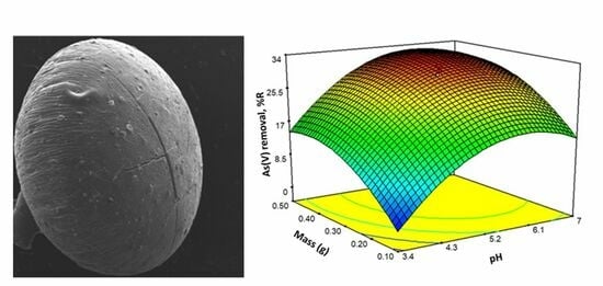
2.2. Scanning Electron Microscope (SEM)

Figure 3 shows the heterogeneity of the chitosan–magnetite spheres and the presence of micro aggregates on their surfaces. It can be seen that the chitosan sphere has portions with layers of different roughness irregularly distributed, Figure 3a. On the other hand, the chitosan spheres with magnetite, Figure 3b, present striations that give them a homogeneous roughness with micro aggregates of particles, while the chitosan–magnetite spheres with As(V) present striations, micro aggregates and an apparent crystallinity, Figure 3c. The latter could indicate that incorporating this element gives it structural rigidity. What is noticeable in both spheres is the portion that corresponds to the zone of detachment or cutting during its synthesis. To develop a more detailed description of the surface of each sphere, different magnifications were applied in different area. These images are consistent with what is reported in the literature for the different materials: chitosan [27] and chitosan–magnetite at the concentration used in this work [28,29,30].

2.3. pH Value at Zero Charge Point (pH_pzc)

The experimentally determined pH_pzc value of the material was 7.21 (Figure 4a); therefore, at a working pH lower than this value, the surface of the sorbent is positively charged. Considering the diagram of As(V) species as a function of pH (Figure 4b), at this pH value the negative H₂AsO₄⁻ species that predominates is the one which is electrostatically attracted to the surface of the sorbent.

2.4. As(V) Detection and Quantification

The concentration of As(V) in the solution was spectrophotometrically determined using the molar absorptivity coefficient determined from the calibration curves performed with the molybdenum blue method, as described in Section 3.3. The value of ε averaged in triplicate was (223,000 ± 100) M⁻¹ cm⁻¹.

The detection limit (LD) is the lowest concentration reliably detectable using the technique. In the modern definition, the detection limit is calculated based on the standard deviation of the predicted concentration for a blank sample [31], Equation (1).

$$\mathrm{s}\left({\mathrm{x}}_{\mathrm{inc}}\right)=\frac{{\mathrm{s}}_{\mathrm{y}/\mathrm{x}}}{\mathrm{A}}\sqrt{\frac{1}{\mathrm{n}}+\frac{1}{\mathrm{m}}+\frac{{({\mathrm{x}}_{\mathrm{inc}}-{\mathrm{x}}_{\mathrm{m}})}^2}{{\mathrm{Q}}_{\mathrm{xx}}}}$$

(1)

where s(x_inc) is the deviation of a x_inc concentration measurement; s_y/x the standard deviation of the regression residuals; n is the number of repetitions of the experiment; m is measured of residues; x_m is the arithmetic mean and A is the slope of linearization. The calculation for Q_xx is shown in Equation (2):

$${\mathrm{Q}}_{\mathrm{x}\mathrm{x}}=\sum _{\mathrm{i}=1}^{\mathrm{m}}{({\mathrm{x}}_{\mathrm{i}}-{\mathrm{x}}_{\mathrm{m}})}^2$$

(2)

If a sample without analyte is analyzed in triplicate (x_inc = 0), Equation (1) reduces to Equation (3):

$$\mathrm{L}\mathrm{D}=3.3\frac{{\mathrm{s}}_{\mathrm{y}/\mathrm{x}}}{\mathrm{A}}\sqrt{\frac{1}{3}+\frac{1}{\mathrm{m}}+\frac{{\left(-{\mathrm{x}}_{\mathrm{m}}\right)}^2}{{\mathrm{Q}}_{\mathrm{x}\mathrm{x}}}}$$

(3)

The LD obtained was 5.27 × 10⁻⁸ M (0.0039 mg L⁻¹ of As(V)). The limit of quantification (LQ) was calculated as indicated using Equation (4) and its value was 1.60 × 10⁻⁷ M (0.012 mg L⁻¹).

$$\mathrm{L}\mathrm{Q}=\frac{\mathrm{L}\mathrm{D}\times 10}{3.3}$$

(4)

2.5. Effect of the Amount of Magnetite on As(V) Sorption

The percentages of As(V) removal using different amounts of magnetite were compared under the same experimental conditions. Figure 5 shows an increase in sorption related to adding magnetite to chitosan. It was decided that we would use 0.5% w/w of magnetite for this work since an increase in the percentage of As(V) removal was observed with the sorbent without magnetite (10%). In contrast, doubling the amount of magnetite increases the removal yield by 3.8%. In addition, a decrease in the mechanical stability of the chitosan–magnetite spheres with 1% magnetite could be observed.

2.6. Experimental Design and Optimization of the Sorption Process

Table 1. Factors calculated using the CCD and the response obtained for each experiment.

Run	pH	Mass (g)	R (%)
1	5.40	0.30	32.00
2	5.40	0.30	30.79
3	2.60	0.30	2.47
4	3.40	0.10	0.01
5	5.40	0.58	33.18
6	7.40	0.50	29.31
7	5.40	0.02	7.80
8	8.20	0.30	15.50
9	3.40	0.50	11.00
10	5.40	0.30	29.86
11	7.40	0.10	16.43

summarizes the values for each factor generated using the Central Composite Design (CCD) and the response obtained experimentally (As(V) removal, R%).

Table 2. ANOVA for Reduced Quadratic model. Response %R.

Source	Sum of Squares	df	Mean Square	F Value	p-Value Prob > F
Reduced quadratic model	1509.95	4	377.49	34.55	0.0003	significant
A-pH	1034.32	1	1034.32	94.67	<0.0001
B-mass	365.46	1	365.46	33.45	0.0012
A2	669.07	1	669.07	61.24	0.0002
B2	169.64	1	169.64	15.53	0.0076
Residual	65.55	6	10.93
Lack of Fit	63.25	4	15.81	13.73	0.0690	not significant
Pure Error	2.30	2	1.15
Cor Total	1575.51	10

shows the Analysis of Variance (ANOVA) analysis for the quadratic model, which best fits the selected response’s experimental data.

From the ANOVA, it is observed that the quadratic model is significant. The factors of pH and mass are significant. The first-order interaction between mass and pH does not significantly influence the response so it was removed from the model. On the other hand, the lack of fit is not significant, indicating the model has a good correlation with the experimental values. The statistical parameters of the model prediction are shown in

Table 3. Statistical parameters of the model prediction.

Std. Dev.	3.31	R2	0.9584
Mean	18.94	Adjusted R2	0.9307
C.V.%	17.45	Predicted R2	0.7988
		Adeq. Precision	14.543

. It is observed that the values of R²-predicted and R²-adjusted did not show a significant difference, which rules out a possible block effect or the presence of outliers within the data set. Adequate precision is related to the signal-to-noise ratio; it is considered correct if its value exceeds 4.

Figure 6 shows the diagnostic plots of the reduced model. These graphs check the assumptions of the model, validating its analysis.

Due to the above, the response (%R) can be expressed through the following mathematical Equation (5), using the encoded coefficients of the model.

$$\%\mathrm{R}=20.81+21.61\mathrm{p}\mathrm{H}+6.82\mathrm{m}\mathrm{a}\mathrm{s}\mathrm{s}-11.03{\mathrm{p}\mathrm{H}}^2-5.55{\mathrm{m}\mathrm{a}\mathrm{s}\mathrm{s}}^2$$

(5)

Positive values of the coefficients imply that an increase in the factor increases the response, and negative values indicate a decrease in the response. In the case of Equation (5), it is observed that the factor with the most significant weight in the %R is the pH. Equation (5) provides the response surface shown in Figure 7.

When the pH increases from 2 to 7, the negatively charged As(V) species increases, Figure 4b. At the same time, the positive charge on the sorbent decreases in that same range (at pH 7.2, the charge is zero), Figure 4a. At a pH close to 6, the combination of factors is optimal for retaining As(V). Increasing the mass to a value of approximately 0.20 g increases the sorption sites and, therefore, the removal of As(V). Above 0.20 g, there is no significant increase in As(V) sorption. This effect may occur because the increase in mass makes it difficult for the contaminant to access.

Optimization of the process under study using the response surface consists of achieving maximum sorption using the minimum amount of sorbent mass, with a pH established in the design range. With these considerations, the model estimated a %R value of 27.61 working at pH 6.00 and 0.22 g of sorbent. Three batch experiments were carried out considering the pH and mass values estimated using the model, preserving the initial conditions with which the complete design experiments were carried out: [As(V)] 2 mg L⁻¹, final volume 25.0 mL, temperature 20 °C and gentle stirring. The following values were obtained for %R: 26.80–27.55–27.70.

2.7. Kinetic Studies

Kinetics experiments were carried out at three temperatures (23 °C, 30 °C and 40 °C) and evaluated using pseudo-first and pseudo-second order models; for each temperature, the amount of contaminant sorbed per gram of sorbent, q_t (mg g⁻¹), was represented as a function of time (min). These results are shown in Figure 8 and

Table 4. Kinetic parameters of the pseudo-first order and pseudo-second order models at 23 °C, 30 °C and 40 °C.

Model	Parameters	23 °C	30 °C	40 °C
pseudo-first order	k1	0.0176 ± 0.0026	0.0228 ± 0.0025	0.0327 ± 0.0033
	%E	14.7	11.0	10.1
	qt %E	1.05 ± 0.03 2.6%	1.25 ± 0.06 4.4%	1.45 ± 0.06 3.8%
	Chi2	0.0001	0.00127	0.0045
	R2	0.9996	0.9943	0.9841
pseudo-second order	k2	0.0093 ± 0.0013	0.0120 ± 0.0016	0.0186 ± 0.0020
	%E	14.0	14.4	10.7
	qt %E	1.50 ± 0.07 8.4%	1.73 ± 0.09 5.4%	1.82 ± 0.060 3.3%
	Chi2	0.0002	0.0009	0.0021
	R2	0.9986	0.9960	0.9926

.

The experimental data fits using the applied kinetic models are both reasonably good. From the statistical parameters and the errors of the constants in Table 4, it cannot be decided whether the model that best describes the process is the pseudo-first order or the pseudo-second order. Using the Arrhenius equation, the values of Activation Energy (E_a) were (28.1 and 31.4) kJ mol⁻¹ using the pseudo-first order or pseudo-second order constants, respectively.

2.8. Thermodynamic Study

A value of q_t (mg g⁻¹) was represented for each temperature as a function of [As(V)] at equilibrium. The Langmuir, Freundlich and Dubinin–Radushkevich models were used. The results obtained are shown below in

Table 5. Thermodynamic parameters for Langmuir, Freundlich and Dubinin Radushkevich models.

Model	23 °C	30 °C	40 °C
Langmuir
qmax(mg g−1)	12.2 ± 1.3	14.0 ± 1.1	15.7 ± 0.6
KLM	3012 ± 275	3593 ± 690	4570 ± 424
R2	0.9957	0.9897	0.9972
Χ2	0.0558	0.1785	0.0577
Freundlich
KF	1.0 ± 0.2	1.0 ± 0.2	0.8 ± 0.2
n	2.1 ± 0.2	2.0 ± 0.2	1.8 ± 0.2
R2	0.9629	0.9785	0.9722
Χ2	0.4631	0.3462	0.5342
Dubinin Radushkevich
qmax(mg g−1)	32.2 ± 3.7	36.2 ± 5.2	46.7 ± 6.7
β(mol2J−2) × 10−9	5.16 ± 0.50	5.20 ± 0.5	5.40 ± 0.46
E(kJ mol−1)	9.77 ± 0.08	8.80 ± 0.05	9.60 ± 0.05
R2	0.9795	0.9854	0.9839

.

The coefficients R² and Χ² suggest that the Langmuir model better fits the experimental data at the studied temperatures, Figure 9. It is also evident that increasing the temperature increases K_LM and the maximum sorption capacity, q_max. This increase may be explained because the sorbent does not have a rigid structure, so the increase in temperature can increase accessibility to the As(V) binding sites. The maximum sorption capacity is located between the values reported in the literature [17,28,29] for the sorption of As(V) with similar sorbents.

The dimensionless constants of the Langmuir model were used to calculate the thermodynamic parameters (∆H° and ∆S°) using Van’t Hoff’s law. The results are shown in Figure 10 and

Table 6. Thermodynamic parameters calculated.

T(K)	KLM (Dimensionless)	ΔG° (kJ mol−1)	ΔH° (kJ mol−1)	ΔS° (J mol−1 K−1)
296	3012	−19.7	16.7	123.3
303	3593	−20.5
313	4570	−21.9

.

For values of E in the (8–16) kJ mol⁻¹ and E_a (24–409) kJ mol⁻¹ ranges, the sorption process is ion exchange. On the other hand, when E is <8 kJ mol⁻¹ and E_a is <40 kJ mol⁻¹, the process is physical. The process is chemical to E > 16 kJ mol⁻¹ and E_a > 40 kJ mol⁻¹ [32]. This work’s E values were (9.8–8.89) kJ mol⁻¹, indicating that the sorption process follows chemical ion exchange. This result agrees with the conclusion obtained in the Arrhenius equation (28.1–31.4) kJ mol⁻¹. The ∆H° value of 16.7 kJ mol⁻¹ indicates the endothermic nature of the As(V) sorption process, and the diffusion from bulk solution to sorbent boundary may involve energy to overcome the interaction of water molecules with As(V) ions. The positive enthalpic change coincides with the increase in the value of the K_LM constant with increasing temperature. It is important to note that as the temperature increases, so does the sorption capacity (q_max), which is consistent with the positive value of ∆H°. The ∆S° value of 123.3 J mol⁻¹ K⁻¹ is positive and is associated with the increase in the system’s disorder during the sorption progression. The ordering produced when the contaminant binds to the sorbent generates a solvent disorder. Finally, the negative ∆G° values confirm the spontaneity of the sorption process under the working conditions used. The process is entropically driven because the T∆S° term is greater than the ∆H° term.

2.9. Desorption Studies

To verify if the sorbent under study can be reused, desorption tests were carried out.

Table 7. The efficiency of the desorption process using different desorbents. Desorbent doses = 0.4 g L⁻¹ and T = 20 °C.

Desorbent	Concentration (M)	Contact Time (h)	D (%)
Na2SO4	1	4	6.68
NaCl	0.5	4	7.14
NaOH	1	4	50.44
NaOH	1	20	84.62

details the results of calculating the efficiency of the desorption process, %D, for each desorbent used.

It can be seen that with the use of 1 M NaOH, better results are obtained than with the other desorbents over the same contact time (4 h). In the case of increasing this time to 20 h, removing As(V) is more efficient, although it has a higher operating cost.

Two more sorption/desorption cycles were realized in the same conditions, yielding removal percentage values of 26% (second cycle) and 24.5% (third cycle), without changing the structure and stability of the sorbent.

3. Materials and Methods

3.1. Obtaining Organic–Inorganic Hybrid Sorbents

The sorbent was prepared as 3.0 mm diameter average size spheres of chitosan–magnetite, as detailed below.

3.1.1. Synthesis of Magnetite

Magnetite Synthesis: 7.84 g of Fe(NH₄)(SO₄)₂·6H₂O and 10.80 g of FeCl₃·6H₂O were weighed to prepare 100 mL of 0.2 M and 0.4 M solution in Fe(II) and Fe(III). To this solution, ammonium hydroxide (20%) was added, with stirring and under a hood, up to pH 9.0, observing the formation of a black suspension that was incubated (80 °C, 30 min), filtered and washed until neutral pH. Work was carried out in an inert nitrogen atmosphere. The solid obtained was dried (60 °C) until at constant weight, homogenized with the help of a mortar and stored in a desiccator. The mass of M obtained was 4.549 g.

Reaction:

Fe(NH₄)₂(SO₄)₂ + 2FeCl₃ + 8NH₄OH → Fe₃O₄ + 4H₂O +2(NH₄)₂SO₄ + 6NH₄Cl

Theoretical mass = 4.64 g; mass obtained = 4.55 g and yield = 98.1%.

3.1.2. Synthesis of Magnetite–Chitosan Spheres

Spheres containing various amounts of magnetite were prepared in the 0.1 and 1% w/w range. For this, 4.0 g of chitosan was dissolved in 100.0 mL of acetic acid (4.0% w/v at 50 °C). The solution was mixed with the desired amounts of magnetite, stirred, and homogenized in a sonicator for one hour. The different mixtures were slowly dripped onto a 2.5 M sodium hydroxide solution with gentle stirring, observing the gelling of the drops as they fell. The obtained spheres were incubated for 24 h in the 2.5 M sodium hydroxide solution, washed with enough distilled water to neutral pH and kept in a refrigerator (4 °C).

3.2. Sorbent Characterization

3.2.1. FT-IR and XRD Spectroscopy

The FT-IR was used to identify the functional chemical groups in the immobilized magnetite–chitosan polymer involved in As(V) sorption. The chitosan–magnetite samples were put in contact with a solution of As(V) 120.0 mg L⁻¹ for 4 h, washed and dried under vacuum for 48 h. A sample of dry spheres without As treatment and chitosan spheres without added magnetite were also used. The samples were prepared according to the KBr 1.5% w/w dilution technique, and spectral scanning was performed in the 400 to 4000 cm⁻¹ range.

The XRD analyses were performed using a Cu Kα (1.5418 Å) source (30 kV, 10 mA) from Bruker D2 Phaser 2nd Generation Diffractometer (Karlsruhe, Germany), with a graphite secondary monochromator and a scintillation counter detector. The powdered sample was placed on a flat plastic plate rotated at 30 rpm. The scans were performed at 25 °C. Time/step: 1.00 s, increment: 0.04° and 2 Theta range: 5–100°.

3.2.2. Scanning Electron Microscope

For the observation and morphological characterization of the sorbent, chitosan, chitosan–magnetite and chitosan–magnetite–As(V), images were taken. For this, an FEI Quanta 200F scanning electron microscope with EDS (Energy Dispersive Spectrometer), ETD (Everhart–Thornley Detector) and BSED (Electron Back Scatter Diffraction) detectors (Instituto Física Rosario, IFIR) were used, which allowed a semi-quantitative elemental analysis to be carried out, achieving textural details and high-resolution topological data, as well as the location of the leading chemical elements of interest. A 15 kV voltage was used with different magnification levels: 240, 800, 3000 and 6000×.

3.2.3. Determination of the pH_pzc

To determine the pH_pzc value, 0.28 g of spheres were placed in 10.0 mL in 0.10 M NaNO₃ solutions adjusted to different pHs in the range of 1.80 to 8.34. The system was stirred for 24 h, and subsequently the pH of the solution was measured again. The difference in pH (∆pH) was calculated by subtracting the initial value from the end [33].

3.3. As(V) Detection and Quantification

As(V) was quantitatively determined using a variant of the classical molybdenum blue method developed in the working group [34]. Different As concentrations were prepared by appropriate dilution from a stock solution of 0.66 mM, using 3.50 mL of 1.0 M HCl and enough distilled water to bring the final volume to 25.00 mL. Finally, the following reagents were added: 0.50 mL of tetrahydrate ammonium heptamolybdate ((NH₄)₆Mo₇O₂₄.4H₂O, 3.0% w/v, Merck, Germany); 1.25 mL of sulfuric acid (H₂SO₄, 14.0% w/v, Cicarelli, pa, Argentine); 0.25 mL of potassium antimony tartrate (C₈H₄K₂O₁₂Sb₂.3H₂O, 0.25% w/v, Cicarelli, pa, Germany) and 0.50 mL of ascorbic acid (C₆H₆O₆, 11% w/v, Biopack, Argentine). Reagents were added in the order indicated. Except for the sulfuric acid solution, the above reagents are unstable over time so they must be prepared on the same day. The final volume of the reaction mixture was 27.50 mL, and the final As(V) concentrations ranged from 6.2 × 10⁻⁸ M to 4.4 × 10⁻⁶ M. Significant redox occurs after adding ascorbic acid, which reduces the molybdate to “molybdenum blue”. The resulting mixture was allowed to react for 40 min, and then absorption spectra measurements were performed in the 550–950 nm range. A glass cuvette with an optical path length of 10.0 cm was used for each measurement to increase the method’s sensitivity. The absorbance value of a blank solution was subtracted from each absorbance value for the concentrations under study. The absorbance values at 890 nm were considered for constructing the calibration curves.

3.4. Effect of the Amount of Magnetite on the Sorption of As(V)

The batch was carried out at a fixed pH using spheres with different amounts of magnetite: 0, 0.1, 0.5 and 1% w/v of magnetite in a final volume of 25.0 mL. The total sorbent mass, the As concentration and the pH were 0.43 g, 2.0 mg L⁻¹ and 6.3, respectively.

3.5. Sorption Process Optimization

A CCD optimized the As sorption. The CCD was raised with two factors, sorbent dose and pH, studied at five levels each. The total number of experiments, 11, was obtained from the design’s composition arrangement. For the optimization of the As(V) sorption process in batch, the As(V) removal percentage, defined using Equation (6), was considered as a response.

$$\%\mathrm{R}=\frac{{{\mathrm{C}}_0-\mathrm{C}}_{\mathrm{f}}}{{\mathrm{C}}_0}\times 100$$

(6)

C₀ is the initial and C_f is the final concentration of As(V), expressed in mg L⁻¹.

To correlate the experimental data and identify the most relevant terms of the model, the second order polynomial equation was used, considering the choice of two factors.

$${\mathrm{y}}_{\mathrm{i}}={\mathsf{\beta }}_0+\sum {\mathsf{\beta }}_1{\mathrm{x}}_{1\mathrm{i}}+\sum {\mathsf{\beta }}_{11}{{\mathrm{x}}_{1\mathrm{i}}}^2+\sum {\mathsf{\beta }}_2{\mathrm{x}}_{2\mathrm{i}}+\sum {\mathsf{\beta }}_{22}{{\mathrm{x}}_{2\mathrm{i}}}^2+\sum {\mathsf{\beta }}_{12}{\mathrm{x}}_{1\mathrm{i}}{\mathrm{x}}_{2\mathrm{i}}+{\mathsf{\epsilon }}_{\mathrm{i}}$$

where y is the response, x₁ and x₂ are the factors, β₀ the constant coefficient and β₁ and β₁₁ the linear and quadratic coefficient, respectively, for one of the factors. β₂ and β₂₂ are the linear and quadratic coefficients of the second factor. β₁₂ is the linear coefficient of the interaction between the factors and ℇ is the model error.

The study of the adjustment of the experimental data for the mathematical model was carried out through the ANOVA. Variance measures the variability, or spread, of a probability distribution. To carry out the optimization, we worked experimentally in a batch at 20 °C. The pH values and sorbent mass ranges were taken as proposed by the design. The ranges of the factors studied were: (0.02–0.58 g) for sorbent mass (0.8–23.2 g L⁻¹), (2.60–8.20) for pH and [As(V)]₀ of 2 mg L⁻¹. The volume used was 25.0 mL with gentle mechanical agitation for 4 h.

3.6. Sorption Kinetic Studies

The kinetic studies were carried out in batches at a controlled temperature of 23 °C, 30 °C and 40 °C and sorbent doses of 17.2 g L⁻¹, pH 6.00 and [As(V)]₀ of 5.0 mg L⁻¹. Sorption kinetics were analyzed with the pseudo-first order or Lagergren model [35] and the pseudo-second order or Ho and McKay model [36].

The pseudo-first order model is commonly used to describe solute sorption from a solution by a solid sorbent. It can be expressed correctly in nonlinear form using Equation (7):

$${\mathrm{q}}_{\mathrm{t}}={\mathrm{q}}_{\mathrm{e}}\left(1-{\mathrm{e}}^{-{\mathrm{k}}_1\mathrm{t}}\right)$$

(7)

and the pseudo-second order equation is defined using Equation (8):

$${\mathrm{q}}_{\mathrm{t}}=\frac{{\mathrm{q}}_{\mathrm{e}}^2{\mathrm{k}}_2\mathrm{t}}{1+{\mathrm{q}}_{\mathrm{e}}{\mathrm{k}}_2\mathrm{t}}$$

(8)

where q_e (mg g⁻¹) and q_t (mg g⁻¹) are the sorption capacity at equilibrium and at any time t, respectively. k₁ and k₂ are the pseudo-first order (min⁻¹) and the pseudo second order rate constants (g mg⁻¹ min⁻¹), respectively. The kinetic data were adjusted using the Sigma Plot 12.0 software. As removal at different contact times (q_t) was calculated using Equation (9):

$${\mathrm{q}}_{\mathrm{t}}=\frac{(\mathrm{C}\mathrm{o}-{\mathrm{C}}_{\mathrm{f}})\mathrm{V}}{\mathrm{s}\mathrm{o}\mathrm{r}\mathrm{b}\mathrm{e}\mathrm{n}\mathrm{t}\mathrm{m}\mathrm{a}\mathrm{s}\mathrm{s}}$$

(9)

where C₀ and C_f are the initial and final As(V) concentrations, respectively, expressed in mg L⁻¹, and V is the volume of the solution in L. The sorbent mass was expressed in g.

3.7. Determination of Activation Energy

The E_a is related to the kinetic constants [37] as observed in Equation (10):

$$\mathrm{k}={\mathrm{A}}_0{\mathrm{e}}^{-{\mathrm{E}}_{\mathrm{a}}/\mathrm{R}\mathrm{T}}$$

(10)

where k is the rate constant of the reaction, A₀ is a temperature-independent factor associated with the frequency of molecular collisions or frequency factor (g mg⁻¹ min⁻¹), E_a is the activation energy required for sorption to occur (kJ mol⁻¹), R the gas constant (8.314 × 10⁻³ kJ mol⁻¹ K⁻¹) and T the absolute temperature (K). The linear form of Equation (11) is the most used.

$$\ln \mathrm{k}=\ln {\mathrm{A}}_0-\frac{{\mathrm{E}}_{\mathrm{a}}}{\mathrm{R}\mathrm{T}}$$

(11)

The value of the E_a was determined graphically from the slope of the curve ln k as a function of 1/T [37].

3.8. Sorption Isotherms

To thermodynamically describe the process, As(V) sorption isotherms were performed at three temperatures: 23 °C, 30 °C and 40 °C. The experiments were carried out with sorbent doses of 17.2 g L⁻¹ and pH 6.00, under constant agitation for 4 h, with arsenic concentrations in the range of 5.0 to 125.0 mg L⁻¹. Metal removal at different contact times (q_t) was calculated using Equation (9). The data obtained were fitted to the Langmuir [38], Freundlich [39] and Dubinin Radushkevich [40] sorption isotherm models using the Sigma Plot 12.0 software. From the data obtained, the thermodynamic parameters of the process were calculated.

3.8.1. Modified Langmuir Model

Recently published works accounted for the abuse and misuse of the Langmuir Model, not only to describe the thermodynamics of the adsorption process in aqueous solutions but also the deduction of the chemical equilibrium constant of the system from the constant of this model [41], which must be dimensionless. Equation (12) shows the modified Langmuir equation:

$${\mathrm{q}}_{\mathrm{e}}=\frac{{\mathrm{q}}_{\mathrm{m}\mathrm{a}\mathrm{x}}{\mathrm{K}}_{\mathrm{L}\mathrm{M}}{\mathrm{C}}_{\mathrm{e}}}{\left({\mathrm{C}}_{\mathrm{s}}-{\mathrm{C}}_{\mathrm{e}}\right)+{\mathrm{K}}_{\mathrm{L}\mathrm{M}}{\mathrm{C}}_{\mathrm{e}}}$$

(12)

It is observed that, regardless of the unit that the adsorbate concentration has, the constant of this model, K_LM, is dimensionless and it is proposed it be use directly without any additional transformation for calculating the thermodynamic variables.

3.8.2. Freundlich Model

The Freundlich equation is one of the first empirical equations used to describe sorption phenomena on heterogeneous surfaces. The model equation is as follows, Equation (13):

$${\mathrm{q}}_{\mathrm{e}}={\mathrm{K}}_{\mathrm{F}}{{\mathrm{C}}_{\mathrm{e}}}^{\left(\raisebox{1ex}{$1$}\!\left/ \!\raisebox{-1ex}{$\mathrm{n}$}\right.\right)}$$

(13)

where q_e (mg g⁻¹) is the amount of sorbate removed at equilibrium, C_e (mg L⁻¹) is the equilibrium sorbate concentration, K_F (mg g⁻¹)/(mg L⁻¹) is the constant of Freundlich, used as an indicator of sorption capacity, and n (dimensionless) is the Freundlich intensity parameter, indicating the magnitude of the driving force of sorption or surface heterogeneity. When n takes values between 1 and 10, the process is said to be favorable [42]. The Freundlich equation is consistent with the thermodynamics of a heterogeneous sorption [43]. The units of K_F depend on the units used for the concentration of the liquid phase (C) and the solid phase (q). The most frequently used units for sorption in aqueous solutions are mg L⁻¹, mmol L⁻¹ (concentrations) or mg g⁻¹, mmol g⁻¹ (q).

3.8.3. Dubinin Radushkevich Model

The Dubinin Radushkevich equation is expressed as follows, Equation (14):

$${\mathrm{q}}_{\mathrm{e}}={\mathrm{q}}_{\mathrm{D}\mathrm{R}}{\mathrm{e}}^{{-\mathrm{K}}_{\mathrm{D}\mathrm{R}}{\mathsf{\epsilon }}^2}$$

(14)

where

$$\mathsf{\epsilon }=\mathrm{R}\mathrm{T}\ln (1+\frac{1}{{\mathrm{C}}_{\mathrm{e}}})$$

(15)

where q_DR (mg g⁻¹) is the adsorption capacity, K_DR (mol² kJ⁻²) is a constant related to the adsorption energy, ε is Polanyi potential, R is the gas constant (8.314 J mol⁻¹ K⁻¹), T is the temperature (K) and q_e is the equilibrium adsorption capacity (mg g⁻¹) for each value of equilibrium adsorbate concentration C_e (mg L⁻¹). It is further defined in Equation (16):

$$\mathrm{E}=\frac{1}{\sqrt{2{\mathrm{K}}_{\mathrm{D}\mathrm{R}}}}$$

(16)

E corresponds to the mean energy of adsorption in units (J mol⁻¹). This isotherm model is often used since the E values can provide information about the adsorption, physical, chemical or ion exchange process. Several authors propose a modification in calculating the Polanyi coefficient contemplating the saturated sorbate concentration in the system (C_s) through Equations (15) and (16) [44,45]

$$\mathsf{\epsilon }=\mathrm{R}\mathrm{T}\ln (1+\frac{{\mathrm{C}}_{\mathrm{s}}}{{\mathrm{C}}_{\mathrm{e}}})$$

(17)

The value $\mathsf{\epsilon }$ will depend on the units in which the concentration C_e is expressed. In addition, working with concentrations close to or far from the saturation of the sorbate under study is different because the fit of this model presents changes in its curvature as the sorbate concentrations approach saturation. Both considerations significantly affect the value of the K_DR parameter related to the sorption mechanism, generating an incorrect interpretation [46]. Equation (17) is used in this work to calculate the Polanyi coefficient as it is considered more appropriate regarding the abovementioned considerations.

3.9. Desorption Studies

To determine if the sorbent can be reused, batch desorption studies were carried out using solutions of different desorbents: 1 M NaOH, 1 M Na₂SO₄ and 0.5 M NaCl. When using 1 M NaOH, we worked with different contact times, 4 and 20 h, to evaluate the desorption efficiency concerning time.

For the evaluation of the efficiency of the desorption process (%D), Equation (18) was applied.

$$\%\mathrm{D}=\frac{{\mathrm{m}}_{\mathrm{d}\mathrm{e}\mathrm{s}}}{{\mathrm{m}}_{\mathrm{s}\mathrm{o}\mathrm{r}\mathrm{b}}}\times 100$$

(18)

where m_des corresponds to the amount of contaminant desorbed (g) and m_sorb is the amount of contaminant contained in the sorbent (g), calculated using the difference between the initial and remaining contaminant in the solution.

The test consisted of loading As(V) on the sorbent, for which a sorbent mass of 20 mg was used, pH 6.00, T 20 °C, initial [As(V)] 50.2 mg L⁻¹ and final volume 67.00 mL, with gentle mechanical agitation for 7 h. After this stage, the spheres were separated from the supernatant and washed with distilled water. The second stage corresponds to desorption under the following experimental conditions: sorbent mass 20 mg (spheres washed from the previous stage), 20 °C, final volume 50.00 mL, adequate volumes of each desorbent and gentle mechanical agitation for 4 h. All assays were performed in duplicate.

Next, two sorption/desorption cycles were carried out, applying the same conditions, to evaluate the removal of As and reusability of the hybrid sorbent.

4. Conclusions

In this work, the main conclusions are the following:

• A chitosan magnetite hybrid sorbent has been synthesized for the remediation of As and characterized using XRD, FT-IR and SEM spectroscopies. The XRD and FT-IR spectroscopy showed the characteristic bands of the components of the hybrid sorbent: magnetite and chitosan. The presence of As on the sorbent is observed in the FT-IR spectrum (521 cm⁻¹) and in the broadening of the bands in XRD.
• The hybrid sorbent has sufficient stability to be used in batches and an adequate retention capacity comparable with similar materials. The pH and mass of magnetite were optimized through experimental designs. The q_max value obtained using equilibrium studies suggests that the sorption process is favorable, in agreement with the thermodynamics parameters.
• The sorption end activation energy indicates that the sorption mechanism is chemical ion exchange.
• The value of q_max increases with increasing temperature according to the endothermic nature of the sorption process.
• The hybrid sorbent has sufficient stability to be used in batches in three sorption/desorption cycles without modifying its structure and integrity, yielding similar removal percentages.
• From an environmental point of view, we highlight the use of environmentally friendly sorbents for As(V) sorption and an inexpensive and straightforward spectrophotometric method with an appropriate sensitivity, limit detection and quantification.
• This work can be described as a starting point for removing arsenic, combining the elimination process of the contaminant with a simple analytical methodology for As determination that can be applied to assist the country’s most deprived areas. This is the primary purpose of this research.

Finally, we must consider that in this study the sorbent used has a simple, economical and ecologically compatible synthesis. The mechanical and chemical stability of the sorbent was high since it could be demonstrated that in four sorption/desorption cycles it retained its retention capacity, the spheres did not degrade, they could be easily and quickly separated from the system and no Fe was found in solution. The times necessary to reach equilibrium with the contaminant were short at room temperature and pH close to 7. Ultimately, the valorization of a remediation process must be compatible with the cost of synthesis of the sorbent, the sorption/desorption time (reuse), process performance and eco compatibility.

References and Notes

1. International Agency for Research on Cancer (IARC). Some Drinking-Water Disinfectants and Contaminants, Including Arsenic. IARC Monographs on the Evaluation of Carcinogenic Risks to Humans 84; World Health Organization: Lyon, France, 2004; Volume 84, pp. 1–477. [Google Scholar]
2. Risk Information System Division. United States Environmental Protection Agency (USEPA). Arsenic, Inorganic (CASRN 7440-38-2). Integrated Risk Information System (IRIS) U.S. Environmental Protection Agency Chemical, Assessment Summary, National Center for Environmental Assessment. 1998. Available online: http://cfpub.epa.gov/ncea/iris/iris_documents/documents/subst/0278_summary.pdf (accessed on 25 October 2023).
3. Argos, M.; Kalra, T.; Pierce, B.L.; Chen, Y.; Parvez, F.; Islam, T.; Ahmed, A.; Hasan, R.; Hasan, K.; Sarwar, G.; et al. A prospective study of arsenic exposure from drinking water and incidence of skin lesions in Bangladesh. Am. J. Epidemiol. 2011, 174, 185–194. [Google Scholar] [CrossRef]
4. Marshall, G.; Ferreccio, C.; Yuan, Y.; Bates, M.N.; Steinmaus, C.; Selvin, S.; Liaw, J.; Smith, A.H. Fifty-Year study of lung and bladder cancer mortality in Chile related to arsenic in drinking water. J. Natl. Cancer Inst. 2007, 99, 920–928. [Google Scholar] [CrossRef]
5. Bhattacharya, P.; Claesson, M.; Bundschuh, J.; Sracek, O.; Fagerberg, J.; Jacks, G.; Martin, R.A.; Storniolo, A.d.R.; Thir, J.M. Distribution and mobility of arsenic in the Río Dulce alluvial aquifers in Santiago del Estero Province, Argentina. Sci. Total Environ. 2006, 358, 97–120. [Google Scholar] [CrossRef]
6. Dubey, B.; Solo-Gabriele, H.M.; Townsend, T.G. Quantities of arsenic-treated wood in demolition debris generated by Hurricane Katrina. Environ. Sci. Technol. 2007, 41, 1533–1536. [Google Scholar] [CrossRef] [PubMed]
7. Navas-Acien, A.; Umans, J.G.; Howard, B.V.; Goessler, W.; Francesconi, K.A.; Crainiceanu, C.M.; Silbergeld, E.K.; Guallar, E. Urine arsenic concentrations and species excretion patterns in American Indian communities over a 10-year period: The strong heart study. Environ. Health Perspect. 2009, 117, 1428–1433. [Google Scholar] [CrossRef]
8. Agency for Toxic Substance and Disease Registry (ATSDR). Toxicological Profile for Arsenic U.S. Department of Health and Humans Services; Public Health Humans Services, Centers for Diseases Control: Washington, DC, USA, 2007. [Google Scholar]
9. Litter, M.I. Actualización. La problemática del arsénico en la Argentina: El HACER. Rev. Soc. Argent. Endocrinol. Ginecol. Reprod. 2010, XVII, 5–10. [Google Scholar]
10. Carrera, A.P.; Cayla, C.; Fabre, J.; Cirelli, A.F. Tecnologías Económicas para el Abatimiento de Arsénico en Aguas January 2010. Available online: https://www.researchgate.net/publication/292257365_Tecnologias_economicas_para_el_abatimiento_de_arsenico_en_aguas/citations (accessed on 25 October 2023).
11. Bardach, A.E.; Ciapponi, A.; Soto, N.; Chaparro, M.R.; Calderon, M.; Briatore, A.; Cadoppi, N.; Tassara, R.; Litter, M.I. Epidemiology of chronic disease related to arsenic in Argentina: A systematic review. Sci. Total Environ. 2015, 538, 802–816. [Google Scholar] [CrossRef] [PubMed]
12. World Health Organization. Guidelines for Drinking-Water Quality, 4th ed.; WHO: Geneva, Switzerland, 2011; p. 564. [Google Scholar]
13. Ning, R.Y. Arsenic removal by reverse osmosis. Desalination 2002, 143, 237–241. [Google Scholar] [CrossRef]
14. Madhura, L.; Kanchi, S.; Sabela, M.I.; Singh, S.; Bisetty, K.; Inamuddin. Membrane technology for water purification. Environ. Chem. Lett. 2018, 16, 343–365. [Google Scholar] [CrossRef]
15. Gabris, M.A.; Rezania, S.; Rafieizonooz, M.; Khankhaje, E.; Devanesan, S.; AlSalhi, M.S.; Aljaafreh, M.J.; Shadravan, A. Chitosan magnetic graphene grafted polyaniline doped with cobalt oxide for removal of Arsenic(V) from water. Environ. Res. 2022, 207, 112209. [Google Scholar] [CrossRef]
16. Jiang, Z.; Li, N.; Li, P.-Y.; Liu, B.; Lai, H.-J.; Jin, T. One-Step Preparation of Chitosan-Based Magnetic Adsorbent and Its Application to the Adsorption of Inorganic Arsenic in Water. Molecules 2021, 26, 1785. [Google Scholar] [CrossRef] [PubMed]
17. Zeng, H.; Sun, S.; Xu, K.; Zhao, W.; Hao, R.; Zhang, J.; Li, D. Adsorption of As(V) by magnetic alginate-chitosan porous beads based on iron sludge. J. Clean. Prod. 2022, 358, 2022. [Google Scholar] [CrossRef]
18. Batistelli, M.; Mora, B.P.; Mangiameli, F.; Mamana, N.; Lopez, G.; Goddio, M.F.; Bellú, S.; González, J.C. A continuous method for arsenic removal from groundwater using hybrid biopolymer-iron-nanoaggregates: Improvement through factorial designs. J. Chem. Technol. Biotechnol. 2021, 96, 923–929. [Google Scholar] [CrossRef]
19. Litter, M.I.; Ingallinella, A.M.; Olmos, V.; Savio, M.; Difeo, G.; Botto, L.; Torres, E.M.F.; Taylor, S.; Frangie, S.; Herkovits, J.; et al. Arsenic in Argentina: Occurrence, human health, legislation and determination. Sci. Total Environ. 2019, 676, 756–766. [Google Scholar] [CrossRef] [PubMed]
20. Lugo-Lugo, V.; Barrera-Díaz, C.; Ureña-Núñez, F.; Bilyeu, B.; Hernández, I. Biosorption of Cr(III) and Fe(III) in single and binary systems onto pretreated orange peel. J. Environ. Manag. 2012, 112, 120–127. [Google Scholar] [CrossRef]
21. Yasmeen, S.; Kabiraz, M.; Saha, B.; Qadir; Gafur; Masum, S. Chromium (VI) Ions Removal from Tannery Effluent using Chitosan-Microcrystalline Cellulose Composite as Adsorbent. Int. Res. J. Pure Appl. Chem. 2016, 10, 1–14. [Google Scholar] [CrossRef]
22. Schwertmann, U.; Cornell, R.M. Iron Oxides in the Laboratory, 2nd ed.; Springer: Berlin/Heidelberg, Germany, 2003. [Google Scholar]
23. Castaldi, P.; Silvetti, M.; Enzo, S.; Melis, P. Study of sorption processes and FT-IR analysis of arsenate sorbed onto red muds (a bauxite ore processing waste). J. Hazard. Mater. 2010, 175, 172–178. [Google Scholar] [CrossRef]
24. Palacios, J.G.; SilvaYumi, M. Síntesis de Nanopartículas de Magnetita Recubiertas de Quitosano para la Adsorción de Cromo Hexavalentel; Escuela Superior Politécnica de Chimborazo: Riobamba, Ecuador, 2023. [Google Scholar]
25. Raz, M.; Moztarzadeh, F.; Hamedani, A.; Ashuri, M.; Tahriri, M. Controlled Synthesis, Characterization and Magnetic Properties of Magnetite (Fe3O4) Nanoparticles without Surfactant under N 2 Gas at Room Temperature. Key Eng. Mater. 2012, 493–494, 746–751. [Google Scholar] [CrossRef]
26. JCPDS file, PDF No. 65-310.
27. de Moraes, M.A.; Cocenza, D.S.; Vasconcellos, F.d.C.; Fraceto, L.F.; Beppu, M.M. Chitosan and alginate biopolymer membranes for remediation of contaminated water with herbicides. J. Environ. Manag. 2013, 131, 222–227. [Google Scholar] [CrossRef]
28. Kloster, G.A.; Londoño, O.M.; Pirota, K.R.; Mosiewicki, M.A.; Marcovich, N.E. Design of super-paramagnetic bilayer films based on chitosan and sodium alginate. Carbohydr. Polym. Technol. Appl. 2021, 2, 100083. [Google Scholar] [CrossRef]
29. Singh, J.; Srivastava, M.; Dutta, J.; Dutta, P. Preparation and properties of hybrid monodispersed magnetic α-Fe2O3 based chitosan nanocomposite film for industrial and biomedical applications. Int. J. Biol. Macromol. 2011, 48, 170–176. [Google Scholar] [CrossRef]
30. Kloster, G.A.; Muraca, D.; Londoño, O.M.; Knobel, M.; Marcovich, N.E.; Mosiewicki, M.A. Structural analysis of magnetic nanocomposites based on chitosan. Polym. Test. 2018, 72, 202–213. [Google Scholar] [CrossRef]
31. Currie, L.A. Detection and quantification limits: Origins and historical overview. Anal. Chim. Acta 1999, 391, 127–134. [Google Scholar] [CrossRef]
32. Inglezakis, V.J.; Zorpas, A.A. Heat of adsorption, adsorption energy and activation energy in adsorption and ion exchange systems. Desalin. Water Treat. 2012, 39, 149–157. [Google Scholar] [CrossRef]
33. Bertoni, F.A.; Medeot, A.C.; González, J.C.; Sala, L.F.; Bellú, S.E. Application of green seaweed biomass for MoVI sorption from contaminated waters. Kinetic, thermodynamic and continuous sorption studies. J. Colloid Interface Sci. 2015, 446, 122–132. [Google Scholar] [CrossRef]
34. Mora, B.E.P.; E Bellú, S.; Mangiameli, M.F.; I García, S.; González, J.C. Optimization of continuous arsenic biosorption present in natural contaminated groundwater. J. Chem. Technol. Biotechnol. 2019, 94, 547–555. [Google Scholar] [CrossRef]
35. Zur Lagergren, S. Theorie der sogenannten adsorption gelöster stoffe. Kungliga Svenska Vetenskapsakademiens. Handlingar 1898, 24, 1–39. [Google Scholar]
36. Ho, Y.S.; McKay, G. Pseudo-second order model for sorption processes. Process Biochem. 1999, 34, 451–465. [Google Scholar] [CrossRef]
37. Castellan, G.W. Fisicoquímica; Addison-Wesley Iberoamericana: San Juan, Puerto Rico, 1998. [Google Scholar]
38. Langmuir, I. The adsorption of gases on plane surfaces of glass, mica and platinum. J. Am. Chem. Soc. 1918, 40, 1361–1403. [Google Scholar] [CrossRef]
39. Freundlich, H.M.F. Uber die, adsorption in losungen. Z. Phys. Chem. 1906, 57, 385–470. [Google Scholar] [CrossRef]
40. Dubinin, M.M.; Radushkevich, L.V. Equation of the Characteristic Curve of Activated Charcoal Proceedings of the Academy of Sciences. Phys. Chem. Sect. USSR 1947, 55, 331–333. [Google Scholar]
41. Azizian, S.; Eris, S.; Wilson, L.D. Re-evaluation of the century-old Langmuir isotherm for modeling adsorption phenomena in solution. Chem. Phys. 2018, 513, 99–104. [Google Scholar] [CrossRef]
42. Tran, H.N.; You, S.J.; Hosseini-Bandegharaei, A.; Chao, H.P. Mistakes and inconsistencies regarding adsorption of contaminants from aqueous solutions: A critical review. Water Res. 2017, 120, 88–116. [Google Scholar] [CrossRef] [PubMed]
43. Crittenden, J.C.; Trussell, R.R.; Hand, D.W.; Howe, K.J.; Tchobanoglous, G. Introduction to Adsorption Phenomena. In Adsorption, in MWH’s Water Treatment: Principles and Design; John Wiley & Sons: Hoboken, NJ, USA, 2012. [Google Scholar]
44. Abe, M.; Kawashima, K.; Kozawa, K.; Sakai, H.; Kaneko, K. Amination of activated carbon and adsorption characteristics of its aminated surface. Langmuir 2000, 16, 5059–5063. [Google Scholar] [CrossRef]
45. Yang, K.; Zhu, L.; Xing, B. Adsorption of polycyclic aromatic hydrocarbons by carbon nanomaterials. Environ. Sci. Technol. 2006, 40, 1855–1861. [Google Scholar] [CrossRef] [PubMed]
46. Hu, Q.; Zhang, Z. Application of Dubinin–Radushkevich isotherm model at the solid/solution interface: A theoretical analysis. J. Mol. Liq. 2019, 277, 646–648. [Google Scholar] [CrossRef]
Figure 1. (a) Assignment of FT-IR signals of chitosan (black), chitosan–magnetite (red) and chitosan–magnetite–As (green) and (b,c) magnified FT-IR spectra and assignment of the signals of chitosan (black), chitosan–magnetite (red) and chitosan–magnetite–As (green).
Inorganics 11 00428 g001
Figure 2. X-ray powder diffractogram of pure synthesized magnetite, magnetite–chitosan, magnetite–chitosan–As(V) and chitosan.
Inorganics 11 00428 g002
Figure 3. SEM images of: (a) chitosan, (b) chitosan–magnetite and (c) chitosan–magnetite–As(V). ETD detector, 240× magnification.
Inorganics 11 00428 g003
Figure 4. (a) The pHpzc chitosan polymer. Sorbent dose 28 g L−1, NaNO3 0.01 mol L−1, T = 25 °C 24 h equilibrium time and (b) distribution diagram of arsenate species as a function of pH.
Inorganics 11 00428 g004
Figure 5. Effect of magnetite addition on As(V) sorption.
Inorganics 11 00428 g005
Figure 6. Normal probability graphs of studentized (a) residuals and (b) outliers.
Inorganics 11 00428 g006
Figure 7. Response surface generated using Equation (5).
Inorganics 11 00428 g007
Figure 8. Kinetic data and fit employing (a) pseudo-first order and (b) pseudo-second order kinetic model. Sorbent dose = 17.2 g L−1, pH = 6.00 and [As(V)]0 = 5 mg L−1.
Inorganics 11 00428 g008
Figure 9. Sorption isotherm, Langmuir Model of As(V) ions onto chitosan–magnetite. Sorbent doses = 17.2 g L−1; pH = 6.00 and [As(V)]0 = 5–125 mg L−1.
Inorganics 11 00428 g009
Figure 10. Van’t Hoff graph for the determination of the thermodynamic parameters ∆H° and ∆S° of the sorption process.
Inorganics 11 00428 g010