Simulation-Based Optimization of Truck Appointment Systems in Container Terminals: A Dual Transactions Approach with Improved Congestion Factor Representation

Abstract

Background: Container terminals (CTs) have constantly administered truck appointment systems (TASs) to effectively accomplish the planning and scheduling of drayage operations. However, since the operations in the gate and yard area of a CT are stochastic, there is a need to incorporate uncertainty during the development and execution of appointment schedules. Further, the situation is complicated by disruptions in the arrival of external trucks (ETs) during transport, which results in congestion at the port due to unbalanced arrivals. In the wake of Industry 4.0, simulation can be used to test and investigate the present CT configurations for possible improvements. Methods: This paper presents a simulation optimization (SO) and simulation-based optimization (SBO) iteration framework which adopts a dual transactions approach to minimize the gate operation costs and establish the relationship between productivity and service time while considering congestion in the yard area. It integrates the use of both the developed discrete event simulation (DES) and a mixed integer programming (MIP) model from the literature to iteratively generate an improved schedule. The key performance indicators considered include the truck turnaround time (TTT) and the average time the trucks spend at each yard block (YB). The proposed approach was verified using input parameters from the literature. Results: The findings from the SO experiments indicate that, at most, two gates were required to be opened at each time window (TW), yielding an average minimum operating cost of USD 335.31. Meanwhile, results from the SBO iteration experiment indicate an inverse relationship between productivity factor (PF) values and yard crane (YC) service time. Conclusions: Overall, the findings provided an informed understanding of the need for dynamic scheduling of available resources in the yard to cut down on the gate operating costs. Further, the presented two methodologies can be incorporated with Industry 4.0 technologies to design digital twins for use in conventional CT by planners at an operational level as a decision-support tool.

1. Introduction

The global supply chain has become increasingly reliant on maritime transport due to the expansion of the world economy and the rapid increase in international trade. Despite the COVID-19 pandemic’s effects, which reduced global trade, the world economy began to recover in 2021 mainly because consumer spending grew due to the relaxation of pandemic-related restrictions [1]. The global containerized trade rebounded and reached a mark of close to 165 million TEU in 2021 [2]. It declined slightly by −0.7% in 2022 and was forecasted to grow to 1.2% in 2023, as shown in Figure 1 below.

Numerous seaports are currently facing the challenge of dealing with significant truck influxes and congestion at terminal gates [3]. The circumstance mentioned above gives rise to extended vehicle queues, thereby impeding the terminal’s operational effectiveness and resulting in significant levels of air pollution due to truck idling-related carbon emissions [4].

Since the terminal operator always gives priority service to the berthing vessels and, by extension, to the yard trucks (YTs) responsible for the transfer of containers between the quayside and the yard side, there will always exist an imbalance in the workload distribution [5]. The available YCs that are meant to serve the arriving ETs will not be capable of matching up with the demand corresponding to the arriving ETs at that moment. This results in a workload imbalance, as the YC will be prioritized to serve the YT. Therefore, terminal managers must devise a way to control arrivals and alleviate congestion.

Previous research has reported the use of techniques such as a toll traffic policy [6], vessel-dependent time windows (VDTWs) [7], and TASs [8,9] to manage the above situation. The TAS has been primarily used to effectively manage ET arrivals to eliminate congestion in the yard and at the gate areas of a CT. This results in minimizing the overall costs and environmental emissions from truck idling associated with longer waiting times. Implementing a strategy that allows a given number of trucks into the CT at a specific TW implies that the TAS can reduce the number of trucks meant to arrive at peak hours. Consequently, this approach can enhance the overall efficiency and CT performance.

Terminal managers are entirely responsible for appointment-related decisions to regulate the influx of ETs into the CT. It is imperative to effectively allocate jobs to the available resources during the scheduling process [10,11]. The available resources encompass gate processing stations and yard handling equipment. Nevertheless, the effectiveness of the schedules might be compromised by many uncertainties in the operational processes, such as delays at the gates during truck processing, delays caused by cranes during stacking or unstacking activities, and unforeseen downtimes possibly due to failures and maintenance [12]. Studies related to equipment failures also affirmed the impact of the uncertainties on the overall efficiency of a CT and the need to consider these uncertainties during schedule development and execution. Yu et al. [13] underscored in their study that CT operations were hugely impacted by the aging of the equipment and the high rates of failures. This significantly increased maintenance costs and downtimes, affecting the overall port efficiency. Additionally, a study conducted by Pham and Nguyen [14] on cargo handling equipment used by CTs in Vietnam found that they operated below the intended capacity due to execution ineffectiveness. The frequent downtimes contributed to the underperformance that affected the CT’s throughput and the operations’ efficiency. As much as failure and maintenance are paramount, considering both aspects may increase the complexity of the scheduling models and make it intractable [10].

The dual transactions approach permits an external truck to engage in the pick-up operation of an import container immediately following the completion of a drop-off operation of an export container in a single request [15]. Implementing the approach mentioned above may pose challenges because priority rules for serving trucks based on transaction type are needed. Moreover, it is not sure that the trucking companies (TCs) are willing to engage in collaboration and distribute the benefits among themselves after that. Therefore, it is essential to devise a robust scheduling strategy for ET appointments incorporating single and dual transaction appointments to mitigate CT congestion.

Moreover, prior studies by Azab et al. [16] did not tackle the influence of dynamic factors such as traffic levels on the truck’s travel time during the model formulation, considering that within the CT area lies a road network. They assume that the truck moves seamlessly without encountering any traffic-related delays in the gate and yard areas, accomplishes the assigned tasks in a given time duration, and exits. Using this simplifying assumption will consequently impact the inter-terminal truck travel time and, subsequently, the average TTT. Hence, it is imperative to develop a versatile TAS that can effectively accommodate potential uncertainties during the execution of schedules.

In this paper, we develop a TAS simulation model that leverages dual transactions in a conventional CT for optimization to minimize the cost incurred in opening entry gate counters at each TW of the planning horizon. Further, a simulation-based optimization approach is developed to iteratively improve the schedules obtained from the mathematical optimization model using the simulation output. The model considers results from a clustering process from previous work as the input and yields the average TTT as the output at the end of a multi-replication simulation run.

The rest of the paper is organized as follows: Section 2 presents a literature review, Section 3 presents the problem description and simulation model development, Section 4 and Section 5 describe the case under study and the set-up of the experiments, Section 6 reports the results and analyzes the findings, and Section 7 summarizes with the conclusion.

2. Literature Review

The implementation of a TAS inside CT logistics signifies a significant change driven by the need for operational efficiency, sustainability, and effective resource allocation. The TAS has evolved as a strategic method for addressing the complex difficulties related to truck congestion and resource allocation. It is built upon mathematical models derived from queuing theory, optimization algorithms, and systems dynamics. This literature review aims to systematically investigate the scientific basis and empirical support for implementing a TAS in container terminals.

A summary of the methodological framework for the literature review process is provided below. First, it involved searching through databases, including Scopus, Web of Science, Google Scholar, and IEEE. The keywords applied in the search include truck appointment systems, container terminals, dual transactions, external truck scheduling, and simulation. Secondly, filters were used, such as removing duplicates and eliminating articles without DOI numbers and those not written in English. Lastly, to further refine the search, the articles were sorted according to the relevancy concerning the title and abstract of our study. Forty-six articles were recorded and utilized in this study.

This analysis aimed to provide a comprehensive understanding of the complex relationship between scientific concepts and operational realities in the context of implementing and experiencing the TAS in container terminal logistics. The implementation and continuous improvement of the TAS in the management of truck arrivals have elicited interest among academic researchers. To have a broader perspective and understanding of truck arrival scheduling and optimization, we analyze and discuss previous works based on classifications such as the appointment quota optimization, objectives considered, and methodologies used.

Appointment quota determination involves dividing the operation hours of a CT into time windows (TWs). Interviews were conducted in a real-life CT by Giuliano et al. [17] to gather and analyze data on peak hours. The time intervals were partitioned based on the presence or absence of a bottleneck inside each respective frame. Several regulatory procedures were implemented to promote environmental conservation by incentivizing vehicles to arrive at the terminal gate during peak periods, thus mitigating emissions and air pollution. In addition, a strategy of equitably distributing time slots throughout the working hours of the terminal was implemented by Torkjazi et al. [18] to alleviate congestion in both the hinterland and yard regions.

The concept of VDTW was introduced by Chen et al. [7] as a means to effectively regulate the truck arrival pattern and is mainly dependent on the berthing schedule. Trucks were first categorized into groups and allocated to different time slots, at which point they entered the terminal. All groups were assigned a standard time frame to complete the designated duties for a given vessel. Additionally, Do et al. [19] presented a Limited Entering Time Slots (LETS) method to minimize truck and crane emissions. A mathematical model was built to generate time slots for container pick-up. A DES model was also constructed to estimate both the waiting time and emissions. The simulation-based genetic algorithm (GA) was then employed to acquire a time-slot assignment that was close to the best solution. In addition, the efficient scheduling of the berth and yard resources, as well as adequate container slot planning, was thought of as a crucial factor in the determination of the number of trucks to be handled per time slot [10,20,21,22].

Regarding the methodologies, previous studies have pointed out that the TAS mainly uses mathematical modeling, queuing theory, simulation, and a mix of two methodologies. Phan and Kim [23] introduced a mathematical model that facilitates collaboration between TCs and terminals to establish efficient truck operations and appointment schedules. An iterative communication process between transportation companies and terminals resolved the problem. Moreover, Zehender and Feillet [24] suggested a mixed integer linear programming (MILP) model for integrating straddle carrier allocation. The results were confirmed using a DES model that utilized accurate data from the Grand Port Maritime de Marseille. Additionally, a study of the process of negotiating truck arrival schedules between TCs and port terminals was conducted by Phan and Kim [25]. They presented a methodology for determining appointments by considering various expenditures incurred by trucking companies.

A simulation model was employed by Huynh et al. [26] in another study to analyze the relationship between truck turn time and crane availability and deployment. A DES model built on FlexSim was developed by Huynh [27] to study the impacts of appointment scheduling strategies on resource utilization and truck turnaround time. Additionally, non-stationary queuing models were proposed to obtain estimates of the average queue lengths of trucks at the gate and/or in the yard [8,28]. The method suggested by Azab et al. [16] integrated a simulation model with a mixed integer programming (MIP) model to lower the turnaround times of ETs and the difficulties brought on by delaying those trucks’ arrivals past their preferred arrival times.

From the perspective of the objective function formulated in the TAS implementation, researchers sought to either minimize or maximize the objectives in a manner that favors the stakeholders. They aimed to minimize TTT, truck emissions, transportation costs, energy consumption, waiting queue time, and empty trips, or maximize resource utilization. A time window length that was almost ideal for scheduling the arrival of export containers was provided by Chen and Yang [29]. They considered lowering the overall cost of energy use, waiting time, and driving delay time. Additionally, a binary mathematical model was proposed by Abdelmagid et al. [30] to minimize the costs incurred by TC, including waiting time, demurrage, and container transport-related costs. Further, Torkjazi et al. [18] formulated a mathematical model to determine the ideal appointment TWs considering both the TC’s and the CT’s perspective. They aimed to lower the replacement cost of the appointment time frame, the cost of arriving later than planned, and the cost of waiting in the gate area. Jin et al. [31] presented a green lane allocation framework considering carbon emissions. They developed a non-linear fractional integer optimization model to minimize total gate operation and carbon emission costs. The estimation of the ideal appointment quota for the TASs to maximize the use of terminal resources and customer satisfaction was also taken into consideration by [6,27,32,33].

Of great interest in recently published articles is also the application of machine learning (ML) techniques in the design of TASs to aid in scheduling and resource allocation decisions. A two-phase approach that sought to minimize the number of empty trips and deviations from appointed times in a container terminal was presented by Caballini et al. [34]. The method combining clustering analysis and lexicographical optimization was applied to a real-world case in Italy and Mexico ports. Their results show that the proposed approach yields fewer empty-truck trips with lower average TTTs than the present situation.

A data-driven approach was presented by Sun et al. [35] to tackle the problem of appointment quota optimization in CTs. Regression methods were herein used to obtain a causal relationship between the average TTT and the number of truck arrivals. A robust optimization model that minimizes the average TTT and truck deviation from their preferred arrival time while considering the uncertainty was built to obtain an appointment quota plan. Smart gate data were obtained from a genuine CT in Shenzhen, YT, China. Their findings showed that the proposed approach outperformed the current and conventional stochastic optimization models. Recently, da Silva et al. [36] proposed a method that combined DES and ML to dynamically reschedule the allocation of truck appointments in the TAS using real-time data obtained from smart technologies. Upon the determination of the estimated time to travel (ETT) to the port, it triggered the ML algorithm to predict and classify the truck condition as late, on-schedule, or early based on historical data. Their results indicate significantly reduced, by over 80%, average queue size and waiting times at the entrance of the port gates. The proposed approach also reduced the percentage of trucks attended off-schedule to 19% from close to 52%.

Most publications considered only single transactions in the design of the TAS, i.e., they believe that a trucker reserves a single appointment with the CT to arrive and perform either a single pick-up task or a drop-off and leave. A truck can perform both a drop-off and a pick-up in the same appointment request in dual transactions. TCs are encouraged to perform dual transactions where possible to minimize the costs associated with container delivery and reduce the number of empty truck trips. Considering that the CT is constrained with resources such as storage space and yard handling equipment, it is therefore imperative that the TAS is designed in a manner that is beneficial to both the CT managers and the TCs who are the truck owners.

Li et al. [15] introduced a novel method for handling truck arrivals in CTs when conducting dual transactions. Despite the concurrent use of yard handling equipment, it utilized a bi-objective MIP model for optimal quota appointment allocation. A novel three-level vocation queuing model was suggested to calculate the internal truck and ET queuing times for single or dual operations. The results demonstrated that fewer ETs were conducting dual transactions in the queue, which increased the method’s applicability in real-world operations.

To the best of our knowledge, the use of simulation to design and optimize a TAS for dual transactions has not been addressed adequately in the literature. Our overall contribution to this paper involved the design of a simulation tool with two methodologies that can be used by terminal planners to enhance decision-making in their day-to-day operations. A DES model of a deterministic mathematical optimization model adopted from the literature is developed and used to evaluate the resulting schedules while considering the uncertainties. The developed model allows for single and dual transactions in a single appointment request. The model features dynamic gate resource assignment and varying traffic levels at the CT during each TW. The proposed model is flexible and easy to use, as the input parameters can be adjusted to fit different container terminal configurations. In other simulation models presented in the literature, such as [16,37,38,39,40], the capacity of the resource, which is the parameter under study, is set and fixed at the start of the optimization experiment. In contrast, in the proposed case, a programmatically created schedule that parametrizes the capacity of the gate counters to be opened at specific TWs is developed. This allows the parameter to be changed dynamically during the simulation and subsequently during optimization, thus illustrating its contribution.

Optimization experiments were further performed on the developed model to inform the CT manager of the optimum number of gate counters to make them operational at each TW, which yields minimal gate operation costs with reduced congestion. Lastly, an iteration framework to integrate the adopted mathematical and developed simulation model is proposed to improve the representation of congestion factors in the mathematical model and subsequently establish the relationship between the mathematical optimization model inputs and the simulation model input parameters.

3. Problem Description

In this study, we consider typical export and import drayage operations involving the transfer of shipping containers discharged from the ship to the warehouse in the hinterland, and vice versa, with the help of ETs. Terminal operating systems (TOSs) have been adopted and continuously implemented to manage berth, yard, and gate operations and streamline workflows to boost productivity. The TAS module is used for gate management regarding ET arrival, appointment booking, truck cargo verification, and authorization. This module is crucial because the points of arrival and queuing during pick-up and drop-off processes create bottlenecks, resulting in congestion. The flow management, therefore, must be conducted appropriately.

In a terminal where a TAS manages the arrivals of ETs, truckers are bound to book an appointment before arriving at the CT gate. First, the terminal operator sets an appointment quota for each TW, considering the terminal workload and the available yard handling resources. During the determination of the appointment quota, the terminal operator objectively seeks to maximize the productivity of resources and the number of ETs to be served, minimize ET service time, and reduce gate congestion. The appointments are then uploaded to the TOS website, where the TCs can book the preferred TW slot. To complete the booking process, the trucker is supposed to provide the relevant truck and container information for identification purposes.

If the preferred slot is unavailable for booking, the trucker searches for another available slot. Upon securing an appointment, the trucker can proceed to the CT gate for verification/customs checks and access the yard area to accomplish the scheduled tasks. In scenarios where the CT does not provide for the booking mechanism using the TAS, the truckers are allowed to arrive at the gate and join the queue randomly. However, this may be inconvenient to the truckers as they will spend more time waiting for service, since they will have to wait for the occupied yard handling equipment to be released.

Figure 2 below illustrates the two types of moves conducted by an ET considered in this study, i.e., single and dual transaction truck trips. In a single transaction, an ET such as Truck 1 arrives at the CT with an export container x and proceeds to YB7 for the service of unloading by the rubber-tired gantry crane (RTGC) in the same block, and then travels to the CT exit gate for departure. Similarly, another empty truck can enter the CT, pick up import container y, and depart from the CT. For a dual transaction, an ET such as Truck 2 arrives with two export containers, a and b, drops them at YB8 and YB6 successively, and then moves to YB5 and YB1 to pick up import containers c and d before departing from the CT.

4. Solution Methods

4.1. Case Description

This paper presents a conventional CT with a hypothetical rectangular layout configuration measuring 2500 × 750 pixels, whereby 100 pixels represent 100 m in length. The abstracted operations are limited to the processes at the gate and the yard area. The CT layout comprises single unit entry and exit gates, eight YBs, eight overhead YCs, and a complete road network, as shown in Figure 3 and Figure 4 below. Each gate unit comprises gate counters that the ETs use to gain access to and from the yard area upon arrival at the CT and departure from the CT. Inside the CT lies eight YBs, five of which are used to store the inbound containers and three for storing the outbound type. One YC serves each YB at any given point in time. The cranes are assumed to be of the overhead type and are set to operate within the host YB during the simulation period.

A road network that connects the gate and the yard is designed to provide accessibility. It comprises a two-lane one-way road with intersections at the junctions. A four-lane road is constructed right before the entry gate to guide the arriving trucks to the available gate counter. A similar road configuration is also built at the exit to guide the trucks outside the CT in preparation for departure to the final destination. Stopping lines are placed at a point on each access road that leads to the individual YBs where the tasks are set to be performed. Each YB also has an exchange point where the loading and unloading operations occur before the truck is released. The yard capacity and throughput were not considered since the number of containers to be dropped off and picked up at the yard area during model runtime are known in advance and do not change.

ETs arrive at the CT at random times following a preset arrival schedule. The calling population is assumed to be of a finite queue type. The trucks were modeled to arrive at the CT gate according to a schedule in which their preferred arrival times ought to be a random value within the appointed TW following a uniform probability distribution. The period considered is a 1-day horizon divided into 12 time windows (TWs) of 2 h in length each. The arriving trucks can either perform a dual or single transaction. It is required to determine the average time an ET spends in the CT, starting from when it arrives at the CT gate and joins the gate queue until it accomplishes the tasks and leaves the exit gate, i.e., truck turnaround time.

$$\mathrm{T}\mathrm{T}\mathrm{T}={\mathrm{T}}_{\mathsf{\alpha }}+{\mathrm{T}}_{\mathrm{\beta }}+{\mathrm{T}}_{\mathrm{\gamma }}+{\mathrm{T}}_{\mathrm{\phi }}+{\mathrm{T}}_{\mathrm{\omega }},$$

(1)

where T_α is the time taken at the gate in queue waiting, T_β is the time spent at the gate during processing, T_γ is the time taken to travel to the assigned yard area and join the queue, T_ϕ is the time taken to perform pick-up and or loading tasks (including waiting in the queue for YC service), and T_ω is the time taken to exit the CT upon release by the YC (including travel from the last visited YB to the exit gate and final processing at the counter).

Further, to optimize the model, it is required to determine the possible combination of the number of counters to be opened during every TW in a manner that will result in the minimum cost of gate operations. The total cost of operating the gate units depends on the number of gates opened per TW times the negotiated cost payable to individual gate counter operators per period, plus a cost penalty associated with the TTT measured at the end of a simulation run. The number of gates opened at the exit side is fixed throughout the planning horizon. The processing times at the entry gate are expected to be higher than those at the exit gate due to the time-consuming activities such as customs and documentation checks.

The model input parameters are as shown in

Table 1. Simulation model input parameters.

Gate Parameters
CT gate opening hours	Shift 1: 12:00:00 a.m.–08:00:00 a.m. Shift 2: 08:00:00 a.m.–04:00:00 p.m. Shift 3: 04:00:00 p.m.–12:00:00 a.m.
Truck speed (max)	18 km/h [42]
Entry processing time	TRIA (0.5, 1, 4) minutes [27]
Exit processing time with no survey of container	TRIA (0.02, 0.099, 0.3) minutes [26]
Number of gate counters at Entry	3
Number of gate counters at Exit	3
Yard parameters
Number of import blocks (IB)	5 [43]
Number of export blocks (EB)	3 [43]
Number of Yard Cranes (YC)	8 [43]
Unloading/Loading time	0.26 + LOGN (0.941, 0.519) minutes [27]
Road parameters
Lane width	3.5 m
Number of Gate Entry/Exit lanes	3

below.

4.2. Development of a CT Simulation Model

The subsections below outline the reason behind the choice of the adopted modeling technique, the detailed logic development, and the steps followed in verifying the model.

4.2.1. Justification for Modelling Technique

This paper uses a DES modeling technique because the problem can be conceptualized as process-centered in actual practice. It involves the interaction of entities with resources. In this case, the entities are the trucks, whereas the resources include the gate counters and yard cranes. At any given time, a truck seizes a gate or crane resource, delays while being served, and releases the resource for use by another entity waiting in the queue. The processes involved include truck documentation, customs clearance checks at the gates, and container loading and unloading by the YCs at the yard area.

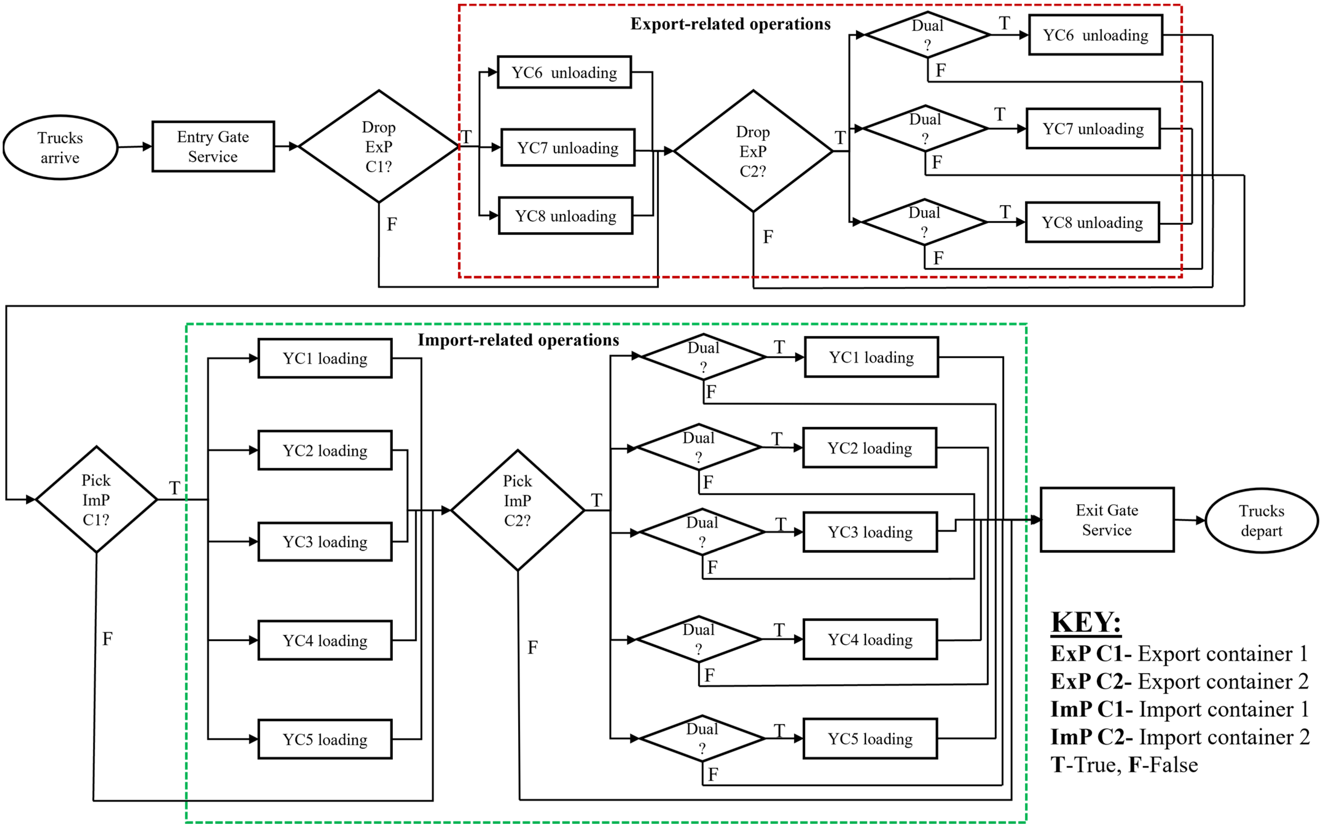
4.2.2. Logic Modeling

The CT simulation model was developed using AnyLogic DES Software—University edition, version 8.8.0. The libraries that were used include Processing Modelling (PML), Material Handling (MHL), and Road Traffic Library (RTL). The process flow chart is constructed using the blocks to capture the occurrence of events sequentially. The blocks utilized from the PML include Resource Pool, Delay, Service, Queue, Hold, Pick-Up, Drop-Off, Select Output, Select Output Out, Select Input In, Move To, Time Measure Start, and Time Measure End. The Move By Crane block is extracted from the MHL, whereas the Car Source, Enter, Exit, Car Move To, and Car Dispose blocks are selected from the RTL.

To visualize the movement of entities inside the model, AnyLogic DES provides 2D and 3D objects and space markup elements. The rectangular and point nodes are used to sketch objects such as the YBs and container exchange points, whereas the Overhead Cranes are used to represent the YCs. Containers and Truck objects are also used to represent the entities interacting in the model. Figure 5 below shows the process flow chart describing the sequence of activities beginning with the trucks’ arrival at the CT, joining the gate queue at the service entry, moving to the yard area for loading/unloading operations, and exiting/departing at the gate.

The order of the activities in the blocks determines the entity’s movement within the model. Before entering the planned YB queue for crane service, the entity (truck) checks against a predetermined condition and goes through the target process if the condition is met. Otherwise, it moves on to the next block until it finds a matching condition, or it leaves the yard area and travels to the exit gate after completing the prescribed operations.

As mentioned in Section 4.1, trucks arrive randomly within the preferred appointed TWs, as shown in

Table 2. Tuple list (ET arrival schedule for the simulation model).

Truck Trip No.	Export	Import	A1	A2	A3	A4	Preferred TW	Priority Index
1	(38, 183)	(385, 652)	8	6	1	5	1	2
2	(190, 299)	(318, 355)	7	7	3	2	1	2
3	(435, 523)	(56, 322)	6	8	2	2	1	2
4	(613, 693)	(16, 238)	8	7	2	2	1	2
1057	(None, None)	(720, None)	0	0	4	0	12	1

. Upon arrival, they are directed to the available gate counter for service. Trucks are served based on the FIFO principle. If all the counters are busy, the arriving trucks join the queue ahead and wait. The tuple list from the previous work conducted by Talaat et al. [41] was generated by data clustering and analysis. It consists of 1057 truck trips of single and dual transaction types and information related to the truck arrival times and YB assignment.

To further describe the shape of the tuple list in Table 2 below, which forms the arrival schedule for the simulation model in this study, reference is made to the first and last rows as examples. A truck in Truck Trip No. 1 is set to arrive at the CT at the preferred TW1 (0000–0200 h) to perform a dual transaction. It is set to drop off two (2) export containers at YB8 and YB6, respectively, and then pick up two (2) import containers at YB1 and YB3, respectively. In that order, the container identification numbers are 38, 183, 385, and 652. Contrary to the above truck trip, Truck Trip No. 1057 involves a single transaction, of only one (1) import container pick up from IB4 at TW12 (2200–2400 h).

4.2.3. Model Verification and Validation

Verification is the procedure that entails making sure that the developed simulation model accurately represents that of the real system, whereas validation involves comparing the simulation model outcomes to those of actual or real systems. A significant amount of effort was put into verifying the CT simulation model for the current system under study before assessing the performances of the scenarios under investigation. Extensive animation, as well as careful trace analyses, were reliably used in a bid to confirm that the system is behaving appropriately as expected. A discussion with the panel of experts from the port logistics industry and academia through conferences, exhibitions, and site visits on the preliminary numerical output results from the analysis further boosted the exercise at hand.

Since the proposed model has various entity types, including trucks and containers, the verification method necessitated tracking down the entities manually to account for every element generated at the source and disposed at sink points of the model. Further, the logic sequence of entities as they move through the different process blocks was monitored at entry and exit using the system.out.print functions as provided by Java during each simulation run.

Before model execution, the model was constantly subjected to debugging analysis to check and fix the abnormalities and errors in the project code and improve the code. This exercise allowed the seamless and smooth execution of the model when running experiments with multiple replications, significantly improving its reliability and dependability in delivering quality output. After the first step of checking the code, the model’s logic and the experiment’s initial conditions were checked to ensure that the model accurately reflected the actual system under study. This would then be followed by manual tracing and the deployment of elaborate animation to visualize and check if the real system was abstracted properly and accurately.

Although we did not use new empirical data, we validated our model by comparing it with the outcomes from a study conducted by Talaat et al. [43]. Additionally, having undertaken a comprehensive literature review, we chose model parameters from multiple well-known and widely accepted sources in the domain of truck appointment scheduling in CTs, which is similar to our study. Specifically, we referred to studies conducted by Huynh et al. [26], Huynh [27], and Azab et al. [42], as shown in Table 1.

5. Experiment Setup

The experiments conducted in this study were carried out on a Precision 7920 Tower desktop with the following specifications: 128 GB RAM, Intel (R) Xeon^® Gold 6230R CPU @ 2.10 GHz 2.10 GHz. The CT gate and yard operations of a one-day planning horizon were simulated based on the data adopted from the literature. The subsequent sections discuss the results and analysis from the simulation optimization and simulation-based optimization iteration experiments.

5.1. Minimizing the Entry Gate Operation Costs via Simulation-Optimization

Simulation optimization (SO) experiments were conducted on the simulation model developed in AnyLogic DES Software—University edition, version 8.8.0, to determine the optimum number of gate counters required to be opened by the CT during each TW, thereby yielding minimum gate operating costs. An extra gate opened during a specific TW of the planning horizon in a manner that will lead to it being underutilized implies hiring an additional employee at an extra cost, which would have been avoided in the first place through informed decisions tied to proper cost analysis.

The SO experiment relies on multiple parameter variation experiments of multiple replications, terminating simulation experiments in the background to achieve its objective. It allows one to observe the effect of random factors in the stochastic models reflected in the simulation output. The parameters to be varied throughout the experiment included the number of gates available at each TW. Throughout the experiment, the number of gate counters opened throughout each TW varied from a minimum of 1 to a maximum of 5, with a step of 1. In the main simulation model, the parameters were first assigned random integer values within the range of 1–5, assuming that the value represents the current number of counters opened at each particular TW.

An objective function was formulated to minimize the total gate operating costs considering the hourly operating cost, the number of gates available, and the measured average TTT at the end of the simulation run. The OF is as shown below:

$$\mathrm{M}\mathrm{i}\mathrm{n}.\mathrm{G}\mathrm{a}\mathrm{t}\mathrm{e} \mathrm{O}\mathrm{p}\mathrm{e}\mathrm{r}\mathrm{a}\mathrm{t}\mathrm{i}\mathrm{o}\mathrm{n} \mathrm{C}\mathrm{o}\mathrm{s}\mathrm{t}\mathrm{s}\left(\mathrm{\$}\right)=\left(\left(\sum _{\mathrm{i}=1}^{12}\mathrm{A}\right)\mathrm{B}+\left(\mathrm{C}\times \mathrm{A}\mathrm{v}\mathrm{e}\mathrm{r}\mathrm{a}\mathrm{g}\mathrm{e} \mathrm{T}\mathrm{T}\mathrm{T}\right)\right)$$

(2)

where A represents the number of gate counters opened at TW_i, B represents the gate counter opening cost per TW, and C represents the penalty cost associated with the average TTT measured at the end of each simulation run. It takes an integer value greater than zero. A higher value of C implies a higher TTT value, meaning that each truck spent a relatively longer time in the CT to accomplish the scheduled tasks, and vice versa. The value may also be thought of as a factor that represents congestion in the CT, and can be varied throughout the experiment to yield a desired cost value.

The first term represents the summation of the number of gates opened at each TW, a parameter in the experiment that is dynamically varied. This was achieved by creating a programmatic schedule that is initialized from a code upon the start of the model. To limit the search space of the solutions for the optimum parameters that give the best OFV, a 2 h TW length was chosen, which offers twelve parameters available for iteration. The gate operation cost term B and the weight value C were assigned arbitrary values of USD 4 and 8, respectively, for verification purposes. They can, however, be substituted with practical values depending on the situations at the CT.

The SO process was manually carried out systematically and interactively over different combinations and iterations considering the unique memory size allocated for the multi-core parallel evaluation. A maximum of 52 cores and up to 256 GB of memory was assigned to the model as the Java heap space during the model execution and subsequent run. The simulation time taken to obtain the OFV was recorded for a unique combination of replication and iteration where it occurred. It was reported as shown in the results in Section 6.1.

The AnyLogic DES software—University edition, version 8.8.0 uses the OptQuest engine to perform optimization. This is an optimization package embedded in the DES software that combines several strategies, such as genetic algorithms, scatter and tabu search, neural networks (NNs), and integer programming (IP) to evaluate optimum solutions for the parameters in the model [44]. It allows the user to set up the optimization experiment and have complete control by offering flexibility in the input of constraints and other requirements that should be checked at either the start or end of the experiment. Further, it provides a good visualization of the changes in the OFV with different iteration and replication values in a graphical and tabular way.

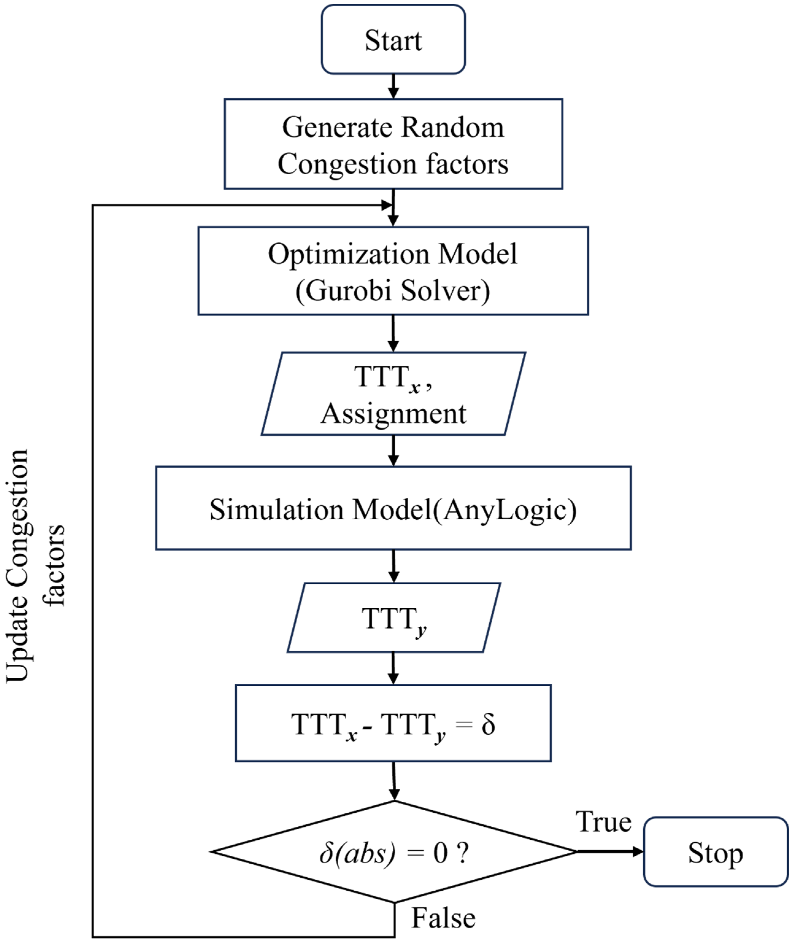
5.2. Improving Congestion Factors Representation through an Iterative Simulation-Based Optimization Procedure

This section involves the proposed integration of the simulation and optimization model. A TAS optimization model proposed by [41] was adopted in this sub-section of the study to implement the proposed integration approach. This approach was conducted to demonstrate that it is indeed possible to link the mathematical model and simulation model in practice and enable them to work simultaneously to enhance the optimization outcomes for prompt and informed decision-making. It is also imperative to note that the mathematical optimization model was implemented in the Gurobi-Python environment and solved using the Gurobi Solver Optimization package V11.0.0, whereas the simulation model was built in the Java environment of the AnyLogic DES software. The integrated approach was carried out manually to verify its practicability.

The simulation-based optimization (SBO) experiment was performed to optimize the assignments generated from the mathematical model and iteratively attempt to improve the solution using the outputs from the developed simulation model. The output from the mathematical model is the assignment and the best OFV. The optimization model function takes randomly generated congestion factors (CFs) and productivity factors (PFs) as the arguments among other inputs, as defined in the literature, and returns the average TTT, denoted by TTT_x, and the arrival schedule, which is an input to the simulation model. A finite horizon simulation experiment was initiated and conducted for Shift 1, and the average TTT_y value was computed.

The results of truck turnaround time and average times spent by a truck in each yard block from the DES model were varied by manually changing the set values of the input parameters (e.g., loading/unloading time) in the Properties tab of the Main simulation panel (AnyLogic environment) for every set of experiments. After every run, the results were exported to Excel and analyzed accordingly. The updated schedules from the adopted TAS optimization model were generated in the Gurobi-Python environment and exported for use in the simulation model as input arrival schedules. The productivity factor and congestion factor matrix values of the mathematical optimization model were manually varied inside the Gurobi-Python interface to yield varying optimized output schedules.

The CF values range from 0.5 to 1, where the lower and higher values correspond to heavy and zero congestion, respectively [34]. The average time spent by the trucks in each block during each TW during each simulation run is also collected and tabulated. The values are then normalized to obtain the updated CF, as mentioned. The updated factors are then fed back to the optimization model to yield new schedules and compute new TTT_x values. The efficiency of the handling equipment in the CT yard is represented by the PF, and it assumes values of 1–6 moves per TW in each YB.

The gap between the two average values is calculated for each iteration to check for possible convergence of the two solutions or improvements in the OFV from the mathematical optimization model. The model is set to stop when the gap is within a set acceptable value, beyond which no further significant improvement can be achieved within the reasonable time equivalent to that required to make a prompt decision. Figure 6 shows a detailed process flow chart describing the proposed approach.

6. Results and Discussions

The following subsections dissect the outcomes of the experiments that were conducted and discuss the potential managerial implications for terminal operators and TCs.

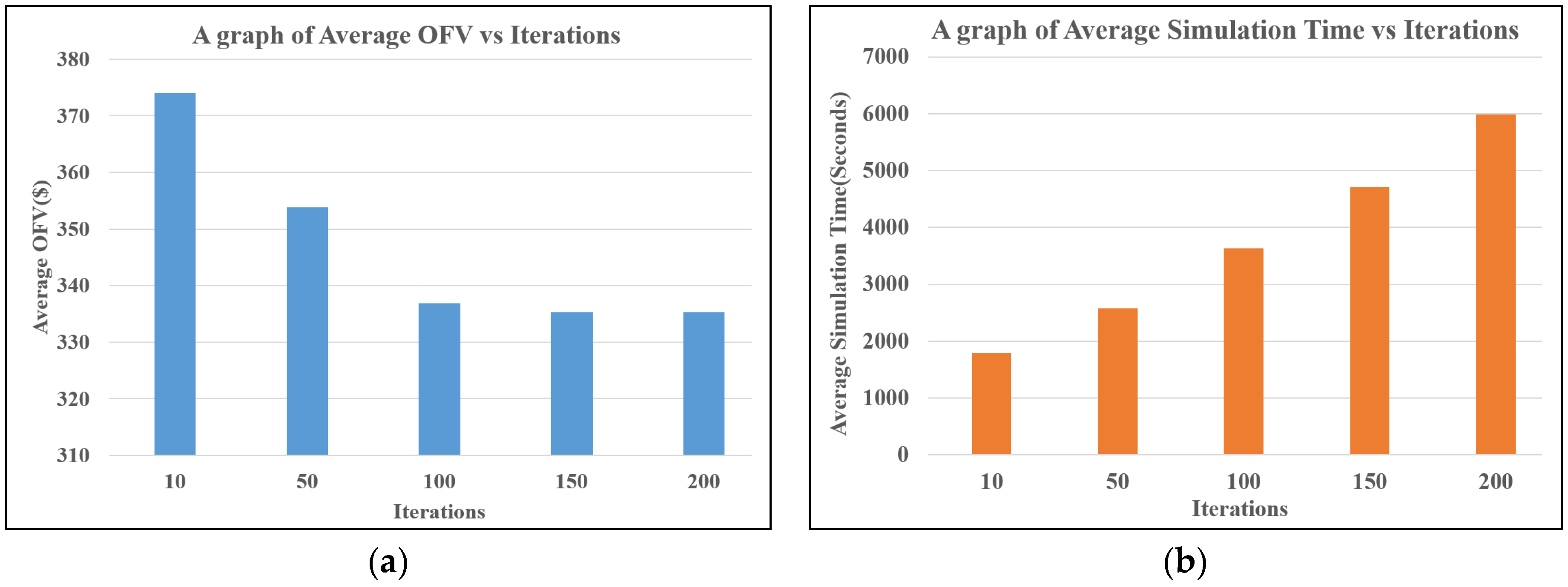
6.1. Simulation Optimization Results

In this section, the findings from the simulation optimization (SO) experiment, as described in Section 5.1, are presented and discussed. The results of the average simulation run time, average OFV, and the gate counters’ combination pattern for each TW for the 10, 50, 100, 150, and 200 iterations are shown in the tables below.

To first determine the necessary number of replications and iterations to conduct the SO experiments, a systematic approach based on the rule of thumb was used to enhance the process. Single SO runs of 5, 10, 15, 20, 25, and 30 replications were first conducted for ten iterations, and the data for the best OFV and simulation time were recorded. Then, the mean values were computed accordingly. The same methodology was replicated for 50, 100, 150, 200, 250, 300, 350, 450, and 500 iterations. The computed average values were tabulated and analyzed, and are represented in the below plots.

From Figure 7a, it can be seen that the average simulation time increases with an increase in the number of iterations. This is an expected phenomenon because the optimization algorithm will take more time while exploring an optimal solution from an ample solution space. In summary, an increase in the iteration counts implies more computations. It is also worth noting in Figure 7b that the algorithm starts to converge at the 200-iteration mark, with slight variation until the 500-iteration mark, where it records the best OFV of USD 335.1 and simulation time of 4552 s as the average. The 200-iteration mark registered the average best OFV and simulation time of USD 335.4 and 3597 s, respectively. From the trend, it is clear that beyond 200 iterations, there may not be a significant improvement in the OFV.

The average simulation time of 3597 s for 200 iterations was subsequently selected to indicate the minimum time required by the CT planner to analyze the submitted appointments by the truckers and provide updated reservation plans. The decision was also supported by the assumed fact that a decision-maker needs to give a solution to an operational problem in a CT in the shortest time possible, it also demands that the solution needs to be better. This, therefore, demonstrates the need to find a tradeoff between the best solution and simulation time, as demonstrated by the percentage difference in

Table 3. Results of OFV over various iterations.

Replications	Number of Iterations
	10	50	100	150	200	250	300	350	400	450	500
	OFV (USD)
5	371.8	339.4	339.3	336.9	335.5	334.7	343.1	336.4	336.6	336.4	335.9
10	375.7	337.0	336.0	334.9	335.6	336.7	335.3	335.8	335.3	335.9	335.2
15	372.5	367.3	340.8	336.8	334.8	335.7	336.3	335.6	336.2	335.0	334.6
20	372.7	358.1	334.4	335.1	336.3	336.3	334.5	336.6	335.1	334.7	334.0
25	371.3	335.7	334.1	335.1	333.9	336.3	332.3	335.1	336.2	335.4	336.5
30	368.3	365.0	336.2	335.6	336.5	335.4	335.3	334.7	335.5	334.6	334.3
Average	372.1	350.4	336.8	335.7	335.4	335.8	336.1	335.7	335.8	335.3	335.1
%Difference	−11.0	−4.6	−0.5	−0.2	−0.1	−0.2	−0.3	−0.2	−0.2	−0.1	0.0

and

Table 4. Results of simulation time over various iterations.

Replications	Number of Iterations
	10	50	100	150	200	250	300	350	400	450	500
	Simulation Time (s)
5	342.7	454.5	562.5	894.4	1037.1	1099.7	1077.8	1184.3	1130.6	1052.1	1184.4
10	658.0	820.0	1234.6	1639.4	2041.5	2446.7	2675.1	2562.1	2475.8	2689.5	2692.3
15	906.7	1319.5	1869.6	2481.5	3021.8	3571.2	4065.4	3795.1	3728.4	4035.8	4036.0
20	1240.0	1759.3	2497.0	3313.1	4006.0	4720.5	5394.3	4986.9	5439.4	5393.0	4935.4
25	1470.5	2093.3	3171.8	4016.6	5182.7	5999.2	7027.9	6733.0	6808.7	6098.6	6072.5
30	1681.5	2470.8	3663.0	4848.6	6292.0	7313.2	7363.8	7606.2	8120.6	8154.7	8391.6
Average	1049.9	1486.2	2166.4	2865.6	3596.9	4191.7	4600.7	4477.9	4617.2	4570.6	4552.0
%Difference	77.3	67.8	53.1	37.9	22.1	9.2	0.4	3.0	0.0	1.0	1.4

below. The managerial implication, in this case, is that because the developed TAS is dynamic and collaborative, the TCs will need to submit the appointments within the stipulated time, and the terminal operator shall immediately analyze the submitted requests and generate the optimized schedules within the CT preferred time (i.e., 1 h). During that time, the TW slots will be frozen and thus unavailable for booking or cancellation.

In Table 3 above, it can be seen that OFV generally decreases with increasing iteration counts while displaying some fluctuations. Additionally, the average OFV value across the iterations stabilizes around 335.1 to 336.8 with minimum variations. A distinct observation of OFV equal to USD 332.3 is noted at replication 25, iteration 300. This is notably lower than other OFVs of higher iterations for the exact replication. This can be attributed to stochastic simulation fluctuations due to inherent randomness and resource constraints or computational issues at specific iteration points. Moreover, the simulation might have reached a temporary optimum state at 300 iterations, which might not have been preserved in the subsequent iterations. The mean and standard deviation (for the OFVs of iterations greater than 300) were calculated and one sample t-test analysis was conducted to investigate further if the value was statistically significant. The mean and standard deviation values of USD 335.8 and 0.66 were obtained, showing that the values were relatively close to each other, whereas a quite high t-statistic value of 10.6 and a significantly lower p-value of 0.00179 (<0.05) were recorded. This preliminarily indicated that randomness might not have been the primary cause of the observed difference.

In Table 4 below, it can be deduced that simulation time increases with an increased number of replications for the different conducted iterations due to increased exploration. Another intriguing observation was made in which the simulation time of 7027.9 s for replication 25, iteration 300 (a similar reference point to that earlier discussed) was recorded. The value is notably higher than for 350, 400, 450, and 500 iterations. In addition to the earlier outlined reasons, the anomaly can be attributed to overfitting, particularly noise, when running many iterations, and potential non-convergence or inconsistent algorithmic behavior. In a similar statistical analysis, a mean and standard deviation value of 6428.2 s and 397 s were obtained, showing that the values were somehow close to each other. In contrast, a t-statistic value of −3.02 and a p-value of 0.057 (>0.05) were recorded. Given a slightly higher p-value, the observed marginal difference was, therefore, not strong enough to rule out variation arising from the inherent randomness.

To further demonstrate the results’ reproducibility, we conducted 30 sets of experiments for each of the 10, 50, 100, 150, and 200 iterations with 30 replications each. We decided not to proceed beyond 200 iterations because, as earlier mentioned, no further significant improvement in the OFV was achieved beyond this point. Moreover, increasing the number of iterations required an increased simulation time for the conducted replications. As seen in Table 3 and Table 4, an additional average time of approximately 16 min is required to realize an improvement of USD 0.3 in the best OFV from 200 to 500 iterations. This can be deemed insignificant considering the significant time and computational effort required in the process vis a vis the traffic congestion, which can build up within a shorter time and cause workload imbalance at the yard and gate areas.

Further, with the advancement in technology, including automation of processes, it is critical to note that decision support systems should be capable of providing solutions in the least time possible so as not to interrupt service delivery, thus creating bottlenecks in resource centers. The results of the best OFV, simulation, and the required optimum gate counter combination are recorded and analyzed as shown in

Table 5. Results of the best OFV, simulation time, and gate counter combination for 200 iterations.

Experiment	Replications	Best OFV (USD)	Simulation Time (s)	Gate Counters Combination
1	(189, 30)	333.92	6161.22	2, 1, 2, 2, 2, 2, 2, 2, 2, 2, 2, 2
2	(154, 30)	335.73	6096.46	2, 2, 2, 2, 2, 2, 2, 2, 2, 2, 2, 2
3	(95, 30)	334.43	5976.64	2, 2, 2, 2, 2, 2, 2, 2, 2, 2, 2, 2
4	(100, 30)	335.65	5797.40	2, 2, 2, 2, 2, 2, 2, 2, 2, 2, 2, 2
5	(87, 30)	336.43	6046.77	2, 2, 2, 2, 2, 2, 2, 2, 2, 2, 2, 2
6	(129, 30)	335.92	5912.67	2, 2, 2, 2, 2, 2, 2, 2, 2, 2, 2, 2
7	(134, 30)	335.24	5918.27	2, 2, 2, 2, 2, 2, 2, 2, 2, 2, 2, 2
8	(95, 30)	336.48	5896.95	2, 2, 2, 2, 2, 2, 2, 2, 2, 2, 2, 2
9	(211, 30)	334.41	5889.97	2, 2, 1, 2, 2, 2, 2, 2, 2, 2, 2, 2
10	(87, 30)	335.88	5972.64	2, 2, 2, 2, 2, 2, 2, 2, 2, 2, 2, 2
11	(93, 30)	336.64	5944.40	2, 2, 2, 2, 2, 2, 2, 2, 2, 2, 2, 2
12	(120, 30)	335.06	5819.81	2, 2, 2, 2, 2, 2, 2, 2, 2, 2, 2, 2
13	(144, 30)	333.71	5824.33	2, 1, 2, 2, 2, 2, 2, 2, 2, 2, 2, 2
14	(95, 30)	336.10	6209.66	2, 2, 2, 2, 2, 2, 2, 2, 2, 2, 2, 2
15	(214, 30)	334.31	5829.35	2, 1, 2, 2, 2, 2, 2, 2, 2, 2, 2, 2
16	(225, 30)	335.90	6082.48	2, 2, 2, 2, 2, 2, 2, 2, 2, 2, 2, 2
17	(181, 30)	334.78	6196.06	2, 1, 2, 1, 2, 2, 2, 2, 2, 2, 2, 2
18	(101, 30)	336.70	5803.55	2, 2, 2, 2, 2, 2, 2, 2, 2, 2, 2, 2
19	(250, 30)	335.61	5842.25	2, 2, 2, 1, 2, 2, 2, 2, 2, 2, 2, 2
20	(158, 30)	335.34	6109.09	2, 2, 2, 2, 2, 2, 2, 2, 2, 2, 2, 2
21	(125, 30)	334.93	5892.40	2, 2, 2, 2, 2, 2, 2, 2, 2, 2, 2, 2
22	(170, 30)	334.64	6067.39	2, 1, 2, 2, 2, 2, 2, 2, 2, 2, 2, 2
23	(131, 30)	335.95	5999.09	2, 2, 2, 2, 2, 2, 2, 2, 2, 2, 2, 2
24	(179, 30)	334.56	6257.06	2, 2, 2, 2, 2, 2, 2, 2, 2, 2, 2, 2
25	(136, 30)	336.43	6038.44	2, 2, 2, 2, 2, 2, 2, 2, 2, 2, 2, 2
26	(139, 30)	333.86	6139.11	2, 1, 2, 2, 2, 2, 2, 2, 2, 2, 2, 2
27	(123, 30)	336.31	6041.06	2, 2, 2, 2, 2, 2, 2, 2, 2, 2, 2, 2
28	(132, 30)	334.32	6044.44	2, 1, 2, 2, 2, 2, 2, 2, 2, 2, 2, 2
29	(205, 30)	334.52	5954.31	2, 1, 2, 2, 2, 2, 2, 2, 2, 2, 2, 2
30	(168, 30)	335.55	6046.86	2, 2, 2, 2, 2, 2, 2, 2, 2, 2, 2, 2
Average		335.31	5993.67

(below), and

Table A1. Results of best OFV, simulation time, and gate counter combination for 10 iterations.

Experiment	Replications	BestOFV (USD)	SimulationTime (s)	Gate Counter Combination
1	(19, 30)	373.54	1739.80	1, 2, 1, 4, 2, 5, 3, 3, 2, 2, 3, 3
2	(19, 30)	373.72	1856.70	1, 2, 1, 4, 2, 5, 3, 3, 2, 2, 3, 3
3	(19, 30)	374.13	1815.00	1, 2, 1, 4, 2, 5, 3, 3, 2, 2, 3, 3
4	(19, 30)	373.69	1777.27	1, 2, 1, 4, 2, 5, 3, 3, 2, 2, 3, 3
5	(19, 30)	373.70	1821.33	1, 2, 1, 4, 2, 5, 3, 3, 2, 2, 3, 3
6	(19, 30)	375.43	1805.21	1, 2, 1, 4, 2, 5, 3, 3, 2, 2, 3, 3
7	(19, 30)	374.00	1824.59	1, 2, 1, 4, 2, 5, 3, 3, 2, 2, 3, 3
8	(19, 30)	373.31	1821.63	1, 2, 1, 4, 2, 5, 3, 3, 2, 2, 3, 3
9	(19, 30)	373.36	1811.09	1, 2, 1, 4, 2, 5, 3, 3, 2, 2, 3, 3
10	(19, 30)	373.72	1805.54	1, 2, 1, 4, 2, 5, 3, 3, 2, 2, 3, 3
11	(19, 30)	374.65	1774.28	1, 2, 1, 4, 2, 5, 3, 3, 2, 2, 3, 3
12	(19, 30)	373.34	1803.41	1, 2, 1, 4, 2, 5, 3, 3, 2, 2, 3, 3
13	(19, 30)	374.08	1798.17	1, 2, 1, 4, 2, 5, 3, 3, 2, 2, 3, 3
14	(19, 30)	372.98	1780.49	1, 2, 1, 4, 2, 5, 3, 3, 2, 2, 3, 3
15	(19, 30)	374.23	1803.28	1, 2, 1, 4, 2, 5, 3, 3, 2, 2, 3, 3
16	(19, 30)	373.74	1778.78	1, 2, 1, 4, 2, 5, 3, 3, 2, 2, 3, 3
17	(19, 30)	374.45	1827.72	1, 2, 1, 4, 2, 5, 3, 3, 2, 2, 3, 3
18	(19, 30)	373.93	1812.62	1, 2, 1, 4, 2, 5, 3, 3, 2, 2, 3, 3
19	(19, 30)	374.62	1844.13	1, 2, 1, 4, 2, 5, 3, 3, 2, 2, 3, 3
20	(19, 30)	373.60	1790.92	1, 2, 1, 4, 2, 5, 3, 3, 2, 2, 3, 3
21	(19, 30)	375.46	1814.20	1, 2, 1, 4, 2, 5, 3, 3, 2, 2, 3, 3
22	(19, 30)	373.09	1761.66	1, 2, 1, 4, 2, 5, 3, 3, 2, 2, 3, 3
23	(19, 30)	372.64	1783.81	1, 2, 1, 4, 2, 5, 3, 3, 2, 2, 3, 3
24	(19, 30)	373.81	1748.23	1, 2, 1, 4, 2, 5, 3, 3, 2, 2, 3, 3
25	(19, 30)	373.40	1741.08	1, 2, 1, 4, 2, 5, 3, 3, 2, 2, 3, 3
26	(19, 30)	373.18	1749.38	1, 2, 1, 4, 2, 5, 3, 3, 2, 2, 3, 3
27	(19, 30)	376.11	1770.83	1, 2, 1, 4, 2, 5, 3, 3, 2, 2, 3, 3
28	(19, 30)	374.98	1761.61	1, 2, 1, 4, 2, 5, 3, 3, 2, 2, 3, 3
29	(19, 30)	375.24	1739.81	1, 2, 1, 4, 2, 5, 3, 3, 2, 2, 3, 3
30	(19, 30)	375.04	1741.94	1, 2, 1, 4, 2, 5, 3, 3, 2, 2, 3, 3
Average		374.04	1790.15

,

Table A2. Results of best OFV, simulation time, and gate counter combination for 50 iterations.

Experiment	Replications	Best OFV (USD)	Simulation Time (s)	Gate Counter Combination
1	(95, 30)	362.49	2646.70	1, 2, 1, 3, 2, 3, 3, 3, 2, 2, 3, 3
2	(95, 30)	334.39	2614.13	2, 2, 2, 2, 2, 2, 2, 2, 2, 2, 2, 2
3	(89, 30)	335.78	2597.12	2, 2, 2, 2, 2, 2, 2, 2, 2, 2, 2, 2
4	(98, 30)	363.25	2514.51	2, 2, 1, 4, 3, 5, 2, 3, 2, 2, 3, 2
5	(71, 30)	357.33	2555.19	4, 2, 2, 2, 2, 2, 2, 3, 2, 3, 2, 4
6	(95, 30)	335.97	2459.54	2, 2, 2, 2, 2, 2, 2, 2, 2, 2, 2, 2
7	(92, 30)	336.28	2441.23	2, 2, 2, 2, 2, 2, 2, 2, 2, 2, 2, 2
8	(99, 30)	364.43	2581.84	2, 3, 2, 3, 3, 3, 3, 3, 2, 3, 3, 3
9	(95, 30)	334.99	2576.05	2, 2, 2, 2, 2, 2, 2, 2, 2, 2, 2, 2
10	(89, 30)	353.85	2480.84	2, 2, 2, 3, 3, 3, 3, 3, 2, 2, 2, 3
11	(90, 30)	367.23	2558.64	2, 2, 4, 5, 2, 2, 3, 2, 2, 3, 2, 3
12	(97, 30)	360.53	2437.02	2, 2, 1, 3, 2, 5, 3, 3, 2, 2, 3, 2
13	(72, 30)	365.48	2558.09	3, 2, 3, 3, 3, 2, 3, 3, 2, 3, 2, 4
14	(91, 30)	363.80	2583.20	3, 2, 1, 3, 2, 3, 3, 3, 2, 3, 3, 3
15	(87, 30)	362.75	2435.68	2, 2, 1, 4, 2, 4, 3, 3, 2, 2, 3, 3
16	(77, 30)	367.05	2318.36	3, 2, 2, 3, 2, 3, 3, 3, 2, 3, 3, 4
17	(95, 30)	334.99	2408.15	2, 2, 2, 2, 2, 2, 2, 2, 2, 2, 2, 2
18	(97, 30)	364.09	2326.07	2, 2, 1, 4, 3, 5, 2, 3, 2, 2, 3, 2
19	(71, 30)	356.58	2327.95	4, 2, 2, 2, 2, 2, 2, 3, 2, 3, 2, 4
20	(93, 30)	364.35	2371.75	2, 3, 1, 3, 2, 5, 2, 3, 2, 2, 3, 3
21	(95, 30)	336.72	2604.53	2, 2, 2, 2, 2, 2, 2, 2, 2, 2, 2, 2
22	(91, 30)	360.94	2330.55	3, 2, 1, 3, 2, 3, 3, 3, 2, 2, 3, 3
23	(77, 30)	365.05	2313.03	3, 2, 3, 3, 3, 2, 3, 3, 2, 3, 2, 4
24	(99, 30)	363.69	2399.64	2, 2, 2, 3, 2, 5, 3, 3, 2, 2, 3, 3
25	(94, 30)	336.60	3079.78	2, 2, 2, 2, 2, 2, 2, 2, 2, 2, 2, 2
26	(77, 30)	367.67	2639.87	3, 2, 2, 3, 2, 3, 3, 3, 2, 3, 3, 4
27	(90, 30)	364.60	3491.71	2, 3, 2, 3, 3, 3, 3, 3, 2, 3, 3, 3
28	(94, 30)	336.13	2765.46	2, 2, 2, 2, 2, 2, 2, 2, 2, 2, 2, 2
29	(99, 30)	361.83	3332.31	1, 2, 1, 3, 2, 3, 3, 3, 2, 2, 3, 3
30	(94, 30)	335.19	2513.79	2, 2, 2, 2, 2, 2, 2, 2, 2, 2, 2, 2
Average		353.80	2575.42

,

Table A3. Results of best OFV, simulation time, and gate counter combination for 100 iterations.

Experiment	Replications	Best OFV (USD)	Simulation Time (s)	Gate Counter Combination
1	(95, 30)	335.90	3726.29	2, 2, 2, 2, 2, 2, 2, 2, 2, 2, 2, 2
2	(87, 30)	336.33	3711.25	2, 2, 2, 2, 2, 2, 2, 2, 2, 2, 2, 2
3	(140, 30)	334.88	3700.98	2, 1, 2, 2, 2, 2, 2, 2, 2, 2, 2, 2
4	(148, 30)	338.98	3704.93	2, 2, 3, 2, 2, 2, 2, 2, 2, 2, 2, 2
5	(134, 30)	335.56	3592.76	2, 2, 2, 2, 2, 2, 2, 2, 2, 2, 2, 2
6	(94, 30)	334.79	3602.35	2, 2, 2, 2, 2, 2, 2, 2, 2, 2, 2, 2
7	(103, 30)	337.03	3588.44	2, 2, 2, 2, 3, 2, 2, 2, 2, 2, 2, 2
8	(121, 30)	334.16	3570.62	2, 1, 2, 2, 2, 2, 2, 2, 2, 2, 2, 2
9	(94, 30)	336.17	3733.59	2, 2, 2, 2, 2, 2, 2, 2, 2, 2, 2, 2
10	(124, 30)	339.20	3571.49	2, 3, 2, 2, 2, 2, 2, 2, 2, 2, 2, 2
11	(94, 30)	335.30	3521.49	2, 2, 2, 2, 2, 2, 2, 2, 2, 2, 2, 2
12	(95, 30)	335.34	3482.06	2, 2, 2, 2, 2, 2, 2, 2, 2, 2, 2, 2
13	(94, 30)	335.31	3500.91	2, 2, 2, 2, 2, 2, 2, 2, 2, 2, 2, 2
14	(123, 30)	336.68	3722.59	2, 2, 2, 2, 2, 2, 2, 2, 2, 2, 2, 2
15	(122, 30)	339.79	3602.76	2, 3, 2, 2, 2, 2, 2, 2, 2, 2, 2, 2
16	(146, 30)	338.92	3460.91	3, 2, 2, 2, 2, 2, 2, 2, 2, 2, 2, 2
17	(135, 30)	336.76	3609.78	2, 2, 2, 2, 2, 2, 2, 2, 2, 2, 2, 2
18	(102, 30)	336.78	3687.66	2, 2, 2, 2, 3, 2, 2, 2, 2, 2, 2, 2
19	(121, 30)	342.43	3614.87	2, 2, 2, 2, 4, 2, 2, 2, 2, 2, 2, 2
20	(87, 30)	335.67	3755.69	2, 2, 2, 2, 2, 2, 2, 2, 2, 2, 2, 2
21	(150, 30)	339.72	3738.85	2, 2, 3, 2, 2, 2, 2, 2, 2, 2, 2, 2
22	(94, 30)	335.33	3815.82	2, 2, 2, 2, 2, 2, 2, 2, 2, 2, 2, 2
23	(130, 30)	334.68	3665.46	2, 1, 2, 2, 2, 2, 2, 2, 2, 2, 2, 2
24	(95, 30)	334.93	3620.66	2, 2, 2, 2, 2, 2, 2, 2, 2, 2, 2, 2
25	(121, 30)	341.21	3624.38	2, 2, 2, 2, 4, 2, 2, 2, 2, 2, 2, 2
26	(95, 30)	335.90	3533.24	2, 2, 2, 2, 2, 2, 2, 2, 2, 2, 2, 2
27	(134, 30)	339.88	3550.20	2, 2, 3, 2, 2, 2, 2, 2, 2, 2, 2, 2
28	(95, 30)	335.57	3663.92	2, 2, 2, 2, 2, 2, 2, 2, 2, 2, 2, 2
29	(131, 30)	336.13	3737.63	2, 2, 2, 2, 2, 2, 2, 2, 2, 2, 2, 2
30	(151, 30)	336.88	3611.79	2, 2, 2, 3, 2, 3, 3, 3, 2, 3, 3, 4
Average		336.87	3634.11

and

Table A4. Results of best OFV, simulation time, and gate counter combination for 150 iterations.

Experiment	Replications	Best OFV (USD)	Simulation Time (s)	Gate Counter Combination
1	(147, 30)	334.88	4706.09	2, 2, 2, 2, 2, 2, 2, 2, 2, 2, 2, 2
2	(89, 30)	336.15	5021.28	2, 2, 2, 2, 2, 2, 2, 2, 2, 2, 2, 2
3	(167, 30)	334.41	4719.36	2, 2, 2, 2, 2, 2, 2, 2, 2, 2, 2, 2
4	(146, 30)	336.81	4627.15	2, 2, 2, 2, 2, 2, 2, 2, 2, 2, 2, 2
5	(150, 30)	334.30	4837.36	2, 1, 2, 2, 2, 2, 2, 2, 2, 2, 2, 2
6	(94, 30)	335.82	4786.05	2, 2, 2, 2, 2, 2, 2, 2, 2, 2, 2, 2
7	(95, 30)	335.61	4817.81	2, 2, 2, 2, 2, 2, 2, 2, 2, 2, 2, 2
8	(175, 30)	335.91	4654.58	2, 2, 2, 2, 2, 2, 2, 2, 2, 2, 2, 2
9	(180, 30)	335.59	4882.80	2, 2, 2, 2, 2, 2, 2, 2, 2, 2, 2, 2
10	(136, 30)	335.87	4634.39	2, 2, 2, 2, 2, 2, 2, 2, 2, 2, 2, 2
11	(95, 30)	335.46	4876.48	2, 2, 2, 2, 2, 2, 2, 2, 2, 2, 2, 2
12	(159, 30)	334.14	4619.38	2, 1, 2, 2, 2, 2, 2, 2, 2, 2, 2, 2
13	(87, 30)	336.00	4826.03	2, 2, 2, 2, 2, 2, 2, 2, 2, 2, 2, 2
14	(135, 30)	335.22	4495.80	2, 2, 2, 2, 2, 2, 2, 2, 2, 2, 2, 2
15	(119, 30)	334.20	4827.79	2, 2, 2, 2, 2, 2, 2, 2, 2, 2, 2, 2
16	(173, 30)	332.45	4581.92	2, 1, 2, 2, 2, 2, 2, 2, 2, 2, 2, 2
17	(122, 30)	333.62	4869.33	2, 1, 2, 2, 2, 2, 2, 2, 2, 2, 2, 2
18	(175, 30)	335.35	4515.13	2, 2, 2, 2, 2, 2, 2, 2, 2, 2, 2, 2
19	(134, 30)	334.72	4810.52	2, 2, 2, 2, 2, 2, 2, 2, 2, 2, 2, 2
20	(176, 30)	335.89	4863.81	2, 2, 2, 2, 2, 2, 2, 2, 2, 2, 2, 2
21	(87, 30)	334.77	4526.43	2, 2, 2, 2, 2, 2, 2, 2, 2, 2, 2, 2
22	(197, 30)	335.15	4839.62	2, 1, 2, 2, 2, 2, 2, 2, 2, 2, 2, 2
23	(95, 30)	335.21	4525.94	2, 2, 2, 2, 2, 2, 2, 2, 2, 2, 2, 2
24	(176, 30)	334.32	4514.03	2, 1, 2, 2, 2, 2, 2, 2, 2, 2, 2, 2
25	(131, 30)	336.30	4772.11	2, 2, 2, 2, 2, 2, 2, 2, 2, 2, 2, 2
26	(127, 30)	336.08	4483.52	2, 2, 2, 2, 2, 2, 2, 2, 2, 2, 2, 2
27	(166, 30)	340.27	4787.60	2, 2, 3, 2, 2, 2, 2, 2, 2, 2, 2, 2
28	(129, 30)	336.21	4494.32	2, 2, 2, 2, 2, 2, 2, 2, 2, 2, 2, 2
29	(152, 30)	334.19	4837.28	2, 1, 2, 2, 2, 2, 2, 2, 2, 2, 2, 2
30	(128, 30)	335.40	4514.55	2, 2, 2, 2, 2, 2, 2, 2, 2, 2, 2, 2
Average		335.34	4708.95

in Appendix A.

From the tables mentioned above, it is worth noting that some homogeneity exists in the average values of the best OFV across the replications for the different iteration values. This consistent achievement of computed mean values compared to the obtained values indicates the algorithm’s capability to find solutions nearly close to the optimal solution. The relatively significant low variability in the best OFV for each iteration value set further justifies the stability and reliability of the results except for a few cases, which may be attributed to the sensitivity to initial conditions.

It can also be observed that there is evidence of the most likely occurring gate counter combination parameter, which gives the best OFV within the replications in each iteration set except for Table A1. This includes [1, 2, 1, 4, 2, 5, 3, 3, 2, 2, 3, 3] for 10 iterations and [2, 2, 2, 2, 2, 2, 2, 2, 2, 2, 2, 2] for 100, 150, and 200 iterations. The harmony strongly points out that the parameter settings used in the simulation model were robust and practical enough for optimizing the formulated OF. From an optimistic view, the terminal operators are convinced that a maximum of two gate counters were required to be opened at each TW throughout the entire shift plan, assuming that the TC complied with their appointments.

In comparison to previous studies, congestion management issues relating to gate operations in the CT have been addressed using different methodologies. Chamchang and Niyomdecha [40] conducted a simulation study to analyze the impact of the number of gate lanes on the queuing performance of a CT. Results from scenario analysis indicated that adding an extra service lane at the gate was not economically justifiable. Furthermore, Keceli [39] abstracted the gate operations of a multi-purpose terminal and conducted scenario analysis using a simulation model. The gate processing time and gate lanes were varied, i.e., 3–4 for the pre-gate and 4–7 for the main gate. Results showed that to keep the number of trucks waiting at the gate at less than 20, the main gate processing time should be reduced by a third, and the lanes increased, i.e., the pre-gate to 4 and the main gate to 6 or 7. Although a similar direct study (simulation model setup) was not encountered, it is evident from the above that varying the gate lanes has been proven to be a crucial factor of interest in enhancing gate performance and, by extension, operation cost.

Different mathematical models have been additionally proposed to optimize the operation costs at marine terminal gates. Guan and Liu [45] applied a multi-server queuing model with non-linear optimization in a New York/New Jersey port to analyze the congestion while considering the gate operating and truck waiting costs. Results showed that of the six gate lanes, five were required to be available for use. A similar approach to the queuing model with an optimized pooled strategy was presented by Minh and Hyunh [46]. Upon application to a port on the US East Coast, it was found that an optimum of 8 out of the 10 installed gates were needed to be operational. Additionally, while applying a fractional integer programming model to a seaport in China, Jin et al. [31] found that expanding the service gate lanes from 8 to 11 would yield minimum gate operation costs. Unlike the above deterministic cases that considered gate operations only in their analysis, our proposed case addressed stochastic operations at both the gate and yard areas in one model with a FIFO strategy. Therefore, comparing our proposed approach directly to the current models discussed was not possible. Nevertheless, out of the five gate counters, it was found from the optimization experiment that at most two were sufficient to serve the arriving trucks at each TW given the set input parameters. This further highlighted a strong indication of the potential benefits of using optimization to minimize gate operation costs and thus manage congestion at the CT.

The plots in Figure 8a,b depict the trends in the relationships between the computed average OVF and simulation time with the number of iterations for the same number of replications. The average OFV decreases with the increasing number of iterations, which agrees with the convergence curve described earlier in Figure 7b. On the other hand, the average simulation time increases with the increase in the number of iterations, thus indicating a directly proportional relationship as compared to the latter, which is inverse. The higher simulation values signify higher computational resource utilization in the search for improved solutions during every optimization run, which may result from complex optimization tasks.

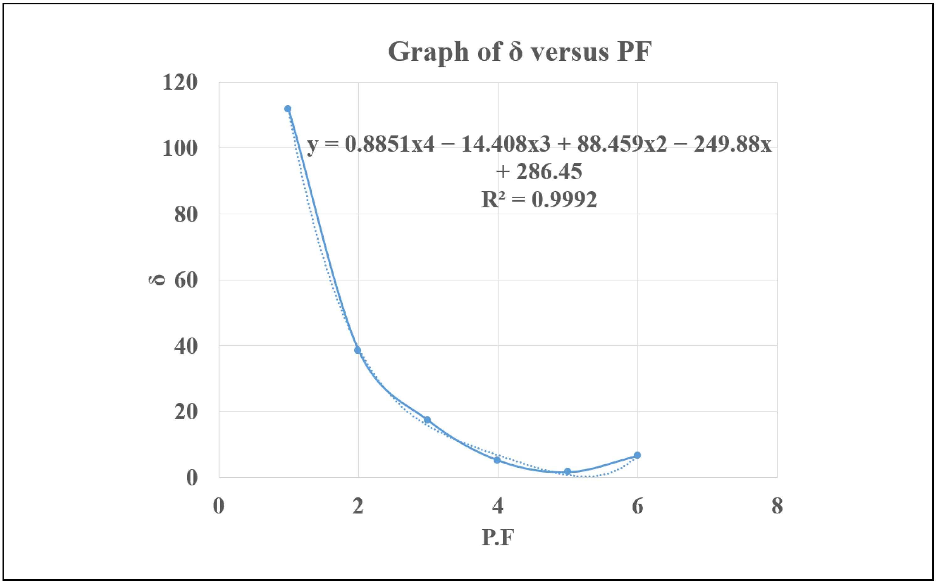
6.2. Simulation-Based Optimization Iteration Results

This section presents the results obtained from the experiments conducted in Section 5.2. It constitutes a dataset from an average of five iterations per run performed for each productivity factor (PF) value ranging from 1 to 6. This makes 30 iterations per run while keeping the yard crane service time in the simulation model constant.

To investigate the relationship between the effect of varying PF values with the YC service time, the YC service time in the AnyLogic simulation model environment is multiplied by factors of 0.5, 1, 1.5, 2.5, 3.5, and 4.5. This makes it a total of 180 iterations. Varying the above loading/unloading time parameter during each run automatically recalculates the required crane parts’ speeds (yard bridge, trolley, and hoist) for each transaction case and, consequently, the handling time of each truck. This directly impacts the time spent by the truck in the yard area during service. Results from the SBO iteration are shown in

Table 6. SBO iteration results of δ and δ (%) for PF = 5.

Iteration	Optimization	Simulation	(TTTx − TTTy)		OFV (∑TTT) Gurobi Solver
	TTTx	TTTy	δ	δ (%)
1	35.35	37.95	−2.60	−7.35	10145.30
2	35.67	38.07	−2.40	−6.74	10235.70
3	34.60	38.04	−3.45	−9.96	9928.31
4	38.10	38.11	−0.01	−0.02	10934.30
5	39.04	38.30	0.74	1.89	11203.20
Average			−1.54	−4.44

(below), and

Table A5. SBO iteration results of δ and δ (%) for PF = 1.

Iteration	Optimization	Simulation	(TTTx − TTTy)		OFV (∑TTT)
	TTTx	TTTy	δ	δ (%)
1	140.89	37.68	103.20	73.25	40,430.40
2	136.80	37.86	98.94	72.33	39,259.30
3	160.88	37.95	122.92	76.41	46,167.10
4	153.20	37.88	115.32	75.27	43,966.00
5	156.22	38.22	118.00	75.53	44,833.20
Average			111.68	74.56

,

Table A6. SBO iteration results of δ and δ (%) for PF = 2.

Iteration	Optimization	Simulation	(TTTx − TTTy)		OFV (∑TTT)
	TTTx	TTTy	δ	δ(%)
1	74.93	37.69	37.24	49.70	21,502.20
2	73.68	37.88	35.80	48.58	21,143.80
3	83.44	37.64	45.80	54.89	23,944.30
4	74.25	37.82	36.43	49.06	21,309.40
5	75.67	37.84	37.83	50.00	21,715.00
Average			38.62	50.45

,

Table A7. SBO iteration results of δ and δ (%) for PF = 3.

Iteration	Optimization	Simulation	(TTTx − TTTy)		OFV (∑TTT)
	TTTx	TTTy	δ	δ (%)
1	52.94	37.99	14.95	28.23	15,192.80
2	53.14	38.18	14.97	28.16	15,250.60
3	56.89	38.09	18.79	33.04	16,324.80
4	55.34	37.58	17.76	32.09	15,881.70
5	57.50	37.66	19.84	34.51	16,499.50
Average			17.26	31.21

,

Table A8. SBO iteration results of δ and δ (%) for PF = 4.

Iteration	Optimization	Simulation	(TTTx − TTTy)		OFV (∑TTT)
	TTTx	TTTy	δ	δ (%)
1	41.95	37.98	3.97	9.46	12,038.10
2	42.08	38.17	3.91	9.30	12,076.90
3	45.34	38.00	7.34	16.20	13,011.20
4	43.75	38.10	5.65	12.92	12,555.50
5	42.80	38.02	4.78	11.16	12,281.40
Average			5.13	11.81

and

Table A9. SBO iteration results of δ and δ (%) for PF = 6.

Iteration	Optimization	Simulation	(TTTx − TTTy)		OFV (∑TTT)
	TTTx	TTTy	δ	δ (%)
1	30.96	38.05	−7.09	−22.92	8883.39
2	31.10	37.90	−6.81	−21.89	8923.53
3	32.30	37.96	−5.67	−17.54	9267.89
4	30.15	38.13	−7.97	−26.44	8653.41
5	32.85	37.85	−5.01	−15.24	9425.66
Average			−6.51	−20.81

of Appendix B.

From the 4th iteration in Table 6 above, it can be observed that an approximate convergence occurs given a PF value of 5. The YC service (loading/unloading) time in the simulation model is kept at T = nTp, as provided in Section 4.1, where n equals 0.5 for the above-presented case. A line plot was drawn to establish the relationship between the absolute value of the gap δ and the PF, as shown in Figure 9 below.

The subsequent plots display the trend of the changes in the relationship between the gap, δ, and PF values when the YC service time is multiplied by the factor n, which equals 1, 1.5, 2.5, 3.5, and 4.5. Each graph displays a polynomial equation fitted to the data points and the corresponding R² value, indicating the goodness of fit. For n = 0.5, 2.5, 3.5, and 4.5, a quartic polynomial fits the data, while for n = 1 and 1.5, a cubic polynomial is used.. The R² values of all the graphs are very high (i.e., close to 1), indicating that the polynomials used fit the data well.

From the plots in Figure 9, Figure 10a,b, Figure 11a,b, and Figure 12a, it can be observed that there is an existence of a downward falling trend at the beginning, followed by a gradual upward rising trend. This is attributed to the approach to and departure from convergence in the value of δ with the increase in the PF values. The convergence point indicates the accurate representation of the practical operations and processes in the mathematical model as it occurs in the CT during the scheduled execution.

For higher n values of 3.5 and 4.5, it can be deduced that the point of convergence is not readily achievable compared to those of 0.5, 1, 1.5, and 2.5, except by interpolation. The curves for n = 2.5, 3.5, and 4.5 seem to display more complexities with the possible occurrence of multiple peaks and valleys representing the inflection points. As seen in Figure 11b and Figure 12a, the trends are characterized by a similar and unique pattern of higher absolute values of δ and more oscillations, suggesting that the relationship between the absolute percentage value of delta and PF may no longer be tenably defined using the provided polynomial equation of the curve. This indicates that the solution from the mathematical model cannot be further effectively improved using the normalized CF values extracted from the simulation model beyond PF values of 2.5.

Consequently, this may be handled by further re-examining the mathematical model, as there might exist other crucial and dependent parameters needed to represent the productivity of the yard handling elements well and which might not have been factored in correctly during the model development in the previous work. This, therefore, forms a basis for our future research.

To further establish the relationship between the PF and the YC service time, the critical points of inflection (x, y), which give the minimum derivative in the fitted curve polynomial, were computed for each of the earlier plotted graphs. The resulting plot is shown in Figure 12b. It can be deduced that an inverse relationship exists between the PF and YC service time. A quadratic polynomial was uniquely selected to fit the polynomial and further present a simplified understanding and interpretation of the overall relationship to the end user.

This graph is essential to a port manager when it comes to the selection of cranes for yard operations. A new crane is likely to achieve better performance with the lowest service time, and vice versa. This is also supported by the fact that higher productivity can be achieved if the YC, during its service, does not waste time dealing with container rehandles. Container pre-marshaling should be done in advance for the formulated container tuples to minimize rehandles, which might lengthen service time and reduce the moves at the YB, thus lowering productivity.

The gap, δ, can also be represented as a percentage change with reference to the TTT value obtained from the mathematical modeling optimization at the end of each iteration. The plots are shown in Figure 13a,b, Figure 14a,b, Figure 15a,b, and Figure 16 below. The major difference in the regression lines in the plots below lies in their polynomial degrees, coefficients, shape, and the range of values they predict. For n = 0.5, 1.5, 2.5, 3.5, and 4.5, a quartic polynomial fits the data, while for n = 1, a quintic polynomial is used. To enhance simplicity and quick understanding for the end user, a quadratic polynomial is used to fit data to describe the relationship between PF and YC service time, as shown in Figure 16.

In summary, the plots presented above display a good fit courtesy of high values of R^2, which are close to 1. The slight variations depict how well the fitted polynomial represents the data variance for each value of n. Higher values of n imply more complex curves characterized by multiple critical points and oscillations. The presented approach is quite similar to that conducted by Azab et al. and Zhou et al. [16,37] in terms of the simulation-based optimization with iteration concept. The methodology proposed by Azab et al. [16] sought to yield an improved collaborative schedule using a single loop, whereas that of Zhou et al. [37] aimed to iteratively improve the allocation decisions of an integrated yard allocation/vehicle congestion problem combined with a heuristic. However, no relationship was reported to have been established between the parameters of the integrated MIP and DES models during the iteration process. As seen in our proposed approach, the output average time spent by the trucks in each yard block during each time window (from each simulation run) was used to iteratively update the input congestion factors for use in the mathematical model, which generates improved arrival schedules (input to the simulation model). Therefore, this study’s contribution lies in improving the representation of congestion factors in the mathematical model through an iterative simulation-based optimization procedure.

7. Conclusions

This paper presents a DES model for use in a conventional CT as a decision support tool during the scheduling of ETs, which are set to arrive and perform container drop-off and pick-up operations in the yard area in either a preferred or appointed time slot. The model allows the arriving ETs to perform a dual transaction in a single trip appointment request, thus increasing utilization and reducing empty trips. SO and SBO iteration experiments were conducted to demonstrate the effectiveness of the developed model on the subsequent performance of the CT. SO was performed to determine the minimum number of gate counters to be opened at each TW for the 24 h shift plan at a minimum gate operating cost. Results from the preliminary systematic approach showed that the optimization algorithm converged at the 200-iteration mark after an average simulation time of up to 3597 s and an average OFV of USD 335.42 as the minimum cost of opening the gates. Furthermore, from the most likely occurring gate counters’ parameter combination in the results of the iteration, it can be observed that a maximum of two gate counters must be operational throughout the planning horizon. Additionally, the optimization results highlight the need to balance the conflicting objectives of the required duration of simulation time and the number of iterations to be conducted in pursuit of an improved OFV. The decision-makers should adopt the best solution achieved in the shortest time possible since ET appointment and scheduling is a dynamic problem, and the TAS should allow for real-time booking and cancellation depending on the prevailing conditions, provided that it jointly favors both stakeholders.

The SBO iteration methodology was also proposed to integrate the mathematical optimization from the literature and the developed CT simulation model in our work. This was done to iteratively improve the arrival schedule using constantly updated CF from the simulation model until a point of convergence in the absolute difference of the average TTT values, δ, from both models is attained. Results from the experiment show that δ decreases with an increase in the PF at the onset, up to the best near convergence point of 0.01 for n equals 0.5, and then increases again for fixed YC service time values. Further, it can be noted that a significant inverse relationship between PF values and YC service time for the values of n equals 0.5, 1, 1.5, and 2.5 can be effectively developed using the approach. The decision-makers can utilize the relationship when selecting a particular crane for a specific task in the yard area while considering the stacking/unstacking and container rehandling time, making up a single or double move. However, for values of n equal to 3.5 and 4.5, it can be noted that the developed relationship, as indicated in the plots, can no longer be relied upon as it does not yield a direct point of convergence. Consequently, the representation of PF and CF in the mathematical model during formulation should be examined and reviewed further in future works. Furthermore, the quayside operations should be incorporated into the proposed approach to enhance integration further and improve coordination among the major sectors/resources providing critical services in a CT. An agent-based simulation model can be further developed to study complex interactions that might arise at a micro-level, e.g., between trucks (internal and external trucks) and resources such as gate counters and yard handling equipment in a practical site. Having conducted an extensive literature review, to the best of our knowledge, no other previous studies considered a similar approach that examined gate counter optimization while considering gate and yard operations simultaneously. This lack of directly comparable studies presents an interesting opportunity for future research. It lays the foundation for further exploitation and comparison as more studies adopt a similar methodology.

References

1. United Nations Conference on Trade and Development (UNCTAD). Review of Maritime Transport. 2022. Available online: https://unctadstat.unctad.org/datacentre/dataviewer/US.TradeMerchGR (accessed on 20 October 2023).
2. United Nations Conference on Trade and Development (UNCTAD). Review Of Maritime Transport. 2023. Available online: https://unctad.org/publication/review-maritime-transport-2023 (accessed on 19 April 2024).
3. Abdelmagid, A.M.; Gheith, M.S.; Eltawil, A.B. A comprehensive review of the truck appointment scheduling models and directions for future research. Transp. Rev. 2022, 42, 102–126. [Google Scholar] [CrossRef]
4. Im, H.; Yu, J.; Lee, C. Truck appointment system for cooperation between the transport companies and the terminal operator at container terminals. Appl. Sci. 2021, 11, 168. [Google Scholar] [CrossRef]
5. Zhang, X.; Zeng, Q.; Yang, Z. Optimization of truck appointments in container terminals. Marit. Econ. Logist. 2019, 21, 125–145. [Google Scholar] [CrossRef]
6. Morais, P.; Lord, E. Terminal Appointment System Study. Transp. Res. Board 2006, 1, 123. [Google Scholar]
7. Chen, G.; Govindan, K.; Yang, Z. Managing truck arrivals with time windows to alleviate gate congestion at container terminals. Int. J. Prod. Econ. 2013, 141, 179–188. [Google Scholar] [CrossRef]
8. Chen, G.; Govindan, K.; Golias, M.M. Reducing truck emissions at container terminals in a low carbon economy: Proposal of a queueing-based bi-objective model for optimizing truck arrival pattern. Transp. Res. Part E Logist. Transp. Rev. 2013, 55, 3–22. [Google Scholar] [CrossRef]
9. Riaventin, V.N.; Cahyono, R.T. Towards Integration of Truck Appointment System and Direction for Future Research. In Proceedings of the 3rd Asia Pacific International Conference on Industrial Engineering and Operations Management, Johor Bahru, Malaysia, 13–15 September 2022; pp. 3022–3030. [Google Scholar] [CrossRef]
10. Oladugba, A.O.; Gheith, M.; Eltawil, A. A new solution approach for the twin yard crane scheduling problem in automated container terminals. Adv. Eng. Inform. 2023, 57, 102015. [Google Scholar] [CrossRef]
11. Doaa, N.; Mohamed, G.; Eltawil, A. A comprehensive review and directions for future research on the integrated scheduling of quay cranes and automated guided vehicles and yard cranes in automated container terminals. Comput. Ind. Eng. 2023, 179, 109149. [Google Scholar] [CrossRef]
12. Bett, D.K.; Ali, I.; Gheith, M.; Eltawil, A. Discrete Event Simulation Of Truck Appointment Systems In Container Terminals: A Dual Transactions Approach. In Proceedings of the International Maritime Transport and Logistics Conference (MARLOG13), Alexandria, Egypt, 2–5 March 2024; pp. 1–16. Available online: https://marlog.aast.edu/files/marlog13/MARLOG13_paper_90.pdf (accessed on 5 May 2024).
13. Yu, H.; Deng, Y.; Zhang, L.; Xiao, X.; Tan, C. Yard Operations and Management in Automated Container Terminals: A Review. Sustainability 2022, 14, 3419. [Google Scholar] [CrossRef]
14. Pham, H.T.; Nguyen, L.H. Empirical Performance Measurement of Cargo Handling Equipment in Vietnam Container Terminals. Logistics 2022, 6, 44. [Google Scholar] [CrossRef]
15. Li, N.; Haralambides, H.; Sheng, H.; Jin, Z. A new vocation queuing model to optimize truck appointments and yard handling-equipment use in dual transactions systems of container terminals. Comput. Ind. Eng. 2022, 169, 108216. [Google Scholar] [CrossRef]
16. Azab, A.; Karam, A.; Eltawil, A. A simulation-based optimization approach for external trucks appointment scheduling in container terminals. Int. J. Model. Simul. 2020, 40, 321–338. [Google Scholar] [CrossRef]
17. Giuliano, G.; O’Brien, T. Reducing port-related truck emissions: The terminal gate appointment system at the Ports of Los Angeles and Long Beach. Transp. Res. Part D Transp. Environ. 2007, 12, 460–473. [Google Scholar] [CrossRef]
18. Torkjazi, M.; Huynh, N.; Shiri, S. Truck appointment systems considering impact to drayage truck tours. Transp. Res. Part E Logist. Transp. Rev. 2018, 116, 208–228. [Google Scholar] [CrossRef]
19. Do, N.A.D.; Nielsen, I.E.; Chen, G.; Nielsen, P. A simulation-based genetic algorithm approach for reducing emissions from import container pick-up operation at container terminal. Ann. Oper. Res. 2016, 242, 285–301. [Google Scholar] [CrossRef]
20. Naeem, D.; Eltawil, A.; Iijima, J.; Gheith, M. Integrated Scheduling of Automated Yard Cranes and Automated Guided Vehicles with Limited Buffer Capacity of Dual-Trolley Quay Cranes in Automated Container Terminals. Logistics 2022, 6, 82. [Google Scholar] [CrossRef]
21. Elwakil, M.; Gheith, M.; Eltawil, A. A New Hybrid Salp Swarm-simulated Annealing Algorithm for the Container Stacking Problem. In Proceedings of the 9th International Conference on Operations Research and Enterprise Systems ICORES, Valetta, Malta, 22–24 February 2020; pp. 89–99. [Google Scholar] [CrossRef]
22. Rashed, D.; Eltawil, A.; Gheith, M. A Fuzzy Logic-Based Algorithm to Solve the Slot Planning Problem in Container Vessels. Logistics 2021, 5, 67. [Google Scholar] [CrossRef]
23. Phan, M.H.; Kim, K.H. Collaborative truck scheduling and appointments for trucking companies and container terminals. Transp. Res. Part B Methodol. 2016, 86, 37–50. [Google Scholar] [CrossRef]
24. Zehendner, E.; Feillet, D. Benefits of a truck appointment system on the service quality of inland transport modes at a multimodal container terminal. Eur. J. Oper. Res. 2014, 235, 461–469. [Google Scholar] [CrossRef]
25. Phan, M.H.; Kim, K.H. Negotiating truck arrival times among trucking companies and a container terminal. Transp. Res. Part E Logist. Transp. Rev. 2015, 75, 132–144. [Google Scholar] [CrossRef]
26. Huynn, N.; Walton, C.M.; Davis, J. Finding the number of yard cranes needed to achieve desired truck turn time at marine container terminals. Transp. Res. Rec. 2004, 1873, 99–108. [Google Scholar] [CrossRef]
27. Huynh, N. Reducing truck turn times at marine terminals with appointment scheduling. Transp. Res. Rec. 2009, 2100, 47–57. [Google Scholar] [CrossRef]
28. Zhang, X.; Zeng, Q.; Chen, W. Optimization Model for Truck Appointment in Container Terminals. Procedia Soc. Behav. Sci. 2013, 96, 1938–1947. [Google Scholar] [CrossRef]
29. Chen, G.; Yang, Z. Optimizing time windows for managing export container arrivals at Chinese container terminals. Marit. Econ. Logist. 2010, 12, 111–126. [Google Scholar] [CrossRef]
30. Abdelmagid, A.M.; Gheith, M.; Eltawil, A. Scheduling External Trucks Appointments in Container Terminals to Minimize Cost and Truck Turnaround Times. Logistics 2022, 6, 45. [Google Scholar] [CrossRef]
31. Jin, Z.; Lin, X.; Zang, L.; Liu, W.; Xiao, X. Lane allocation optimization in container seaport gate system considering carbon emissions. Sustainability 2021, 13, 3628. [Google Scholar] [CrossRef]
32. Schulte, F.; González, R.G.; Voß, S. Reducing port-related truck emissions: Coordinated truck appointments to reduce empty truck trips. In Computational Logistics; Lecture Notes in Computer Science; Springer: Cham, Swizerland, 2015; Volume 9335, pp. 495–509. [Google Scholar] [CrossRef]
33. Schulte, F.; Lalla-Ruiz, E.; González-Ramírez, R.G.; Voß, S. Reducing port-related empty truck emissions: A mathematical approach for truck appointments with collaboration. Transp. Res. Part E Logist. Transp. Rev. 2017, 105, 195–212. [Google Scholar] [CrossRef]
34. Caballini, C.; Gracia, M.D.; Mar-Ortiz, J.; Sacone, S. A combined data mining—Optimization approach to manage trucks operations in container terminals with the use of a TAS: Application to an Italian and a Mexican port. Transp. Res. Part E Logist. Transp. Rev. 2020, 142, 102054. [Google Scholar] [CrossRef]
35. Sun, S.; Zheng, Y.; Dong, Y.; Li, N.; Jin, Z.; Yu, Q. Reducing External Container Trucks’ Turnaround Time in Ports: A Data-driven Approach under Truck Appointment Systems. Comput. Ind. Eng. 2022, 174, 108787. [Google Scholar] [CrossRef]
36. da Silva, M.R.F.; Agostino, I.R.S.; Frazzon, E.M. Integration of machine learning and simulation for dynamic rescheduling in truck appointment systems. Simul. Model. Pract. Theory 2023, 125, 102747. [Google Scholar] [CrossRef]
37. Zhou, C.; Zhao, Q.; Li, H. Simulation optimization iteration approach on traffic integrated yard allocation problem in transshipment terminals. Flex. Serv. Manuf. J. 2021, 33, 663–688. [Google Scholar] [CrossRef]
38. Islam, S. Simulation of truck arrival process at a seaport: Evaluating truck-sharing benefits for empty trips reduction. Int. J. Logist. Res. Appl. 2018, 21, 94–112. [Google Scholar] [CrossRef]
39. Keceli, Y. A simulation model for gate operations in multi-purpose cargo terminals. Marit. Policy Manag. 2016, 43, 945–958. [Google Scholar] [CrossRef]
40. Chamchang, P.; Niyomdecha, H. Impact of service policies on terminal gate efficiency: A simulation approach. Cogent Bus. Manag. 2021, 8, 1975955. [Google Scholar] [CrossRef]
41. Talaat, A.; Iijima, J.; Gheith, M.; Eltawil, A. An Integrated k-Means Clustering and Bi-Objective Optimization Approach for External Trucks Scheduling in Container Terminals. In Advances in Transdisciplinary Engineering; IOS Press BV: Amsterdam, The Netherlands, 2023. [Google Scholar] [CrossRef]
42. Azab, A.; Karam, A.; Eltawil, A. A dynamic and collaborative truck appointment management system in container terminals. In Proceedings of the 6th International Conference on Operations Research and Enterprise Systems ICORES, Porto, Portugal, 23–25 February 2017; pp. 85–95. [Google Scholar] [CrossRef]
43. Talaat, A.; Gheith, M.; Eltawil, A. A Multi-Stage Approach for External Trucks and Yard Cranes Scheduling with CO2 Emissions Considerations in Container Terminals. Logistics 2023, 7, 87. [Google Scholar] [CrossRef]
44. Amaran, S.; Sahinidis, N.V.; Sharda, B.; Bury, S.J. Simulation optimization: A review of algorithms and applications. Ann. Oper. Res. 2016, 240, 351–380. [Google Scholar] [CrossRef]
45. Guan, C.Q.; Liu, R. Modeling gate congestion of marine container terminals, truck waiting cost, and optimization. Transp. Res. Rec. 2009, 2100, 58–67. [Google Scholar] [CrossRef]
46. Minh, C.C.; Huynh, N. Optimal design of container terminal gate layout. Int. J. Shipp. Transp. Logist. 2017, 9, 640–650. [Google Scholar] [CrossRef]
Figure 1. Global containerized trade (1996–2023). Adopted from [2].
Logistics 08 00080 g001
Figure 2. Illustration of single and dual transactions. Adopted from [41].
Logistics 08 00080 g002
Figure 3. A 2D view of the CT gate areas.
Logistics 08 00080 g003
Figure 4. A 2D view of the CT yard area.
Logistics 08 00080 g004
Figure 5. Process flow chart of ET arrival, gate, and yard operations.
Logistics 08 00080 g005
Figure 6. The Proposed simulation-based optimization iteration methodology.
Logistics 08 00080 g006
Figure 7. (a) Graph of average simulation time vs. iterations, (b) graph of average best OFV vs. iterations.
Logistics 08 00080 g007
Figure 8. (a) Average OFV vs. iterations, (b) Average simulation time vs. iterations.
Logistics 08 00080 g008
Figure 9. δ versus PF for n = 0.5.
Logistics 08 00080 g009
Figure 10. (a) δ versus PF for n = 1, (b) δ versus PF for n = 1.5.
Logistics 08 00080 g010
Figure 11. (a) δ versus PF for n = 2.5, (b) δ versus PF for n = 3.5.
Logistics 08 00080 g011
Figure 12. (a) δ versus PF for n = 4.5, (b) PF versus YC service time.
Logistics 08 00080 g012
Figure 13. (a) %δ versus PF for n = 0.5, (b) %δ versus PF for n = 1.
Logistics 08 00080 g013
Figure 14. (a) %δ versus PF for n = 1.5, (b) %δ versus PF for n = 2.5.
Logistics 08 00080 g014
Figure 15. (a) %δ versus PF for n = 3.5, (b) %δ versus PF for n = 4.5.
Logistics 08 00080 g015
Figure 16. PF versus YC service time.
Logistics 08 00080 g016