Abstract
Fine particulate matter (PM2.5) and Ozone (O3) pollution have emerged as the primary environmental challenges in China in recent years. Following the implementation of the Air Pollution Prevention and Control Action Plan, a substantial decline in PM2.5 concentrations was observed, while O3 concentrations exhibited an increasing trend across the country. Here, we investigated the long-term trend of O3 from 2015 to 2022 in Xinxiang City, a typical city within the Central Plains urban agglomeration. Our findings indicate that the hourly average O3 increased by 3.41 μg m−3 yr−1, with the trend characterized by two distinct phases (Phase I, 2015–2018; Phase II, 2019–2022). Interestingly, the increasing rate of O3 concentration in Phase I (7.89 μg m−3) was notably higher than that in Phase II (2.89 μg m−3). The Random Forest (RF) model was employed to identify the key factors influencing O3 concentrations during the two phases. The significant dropping of PM2.5 in Phase I could be responsible for the O3 increase. In Phase II, the reductions in nitrogen dioxide (NO2) and unfavorable meteorological conditions were the major drivers of the continued increase in O3. The Observation-Based Model (OBM) was developed to further explore the role of PM2.5 in O3 formation. Our results suggest that PM2.5 can influence O3 concentrations and the chemical sensitivity regime through heterogeneous reactions and changes in photolysis rates. In addition, the relatively high concentration of PM2.5 in Xinxiang City in recent years underscores its significant role in O3 formation. Future efforts should focus on the joint control of PM2.5 and O3 to improve air quality in the Central Plains urban agglomeration.
1. Introduction
Tropospheric Ozone (O3) is a typical secondary gaseous pollutant and the third most significant greenhouse gas (IPCC, 2021). It has a profound impact on human health, ecosystem stability, and vegetation productivity [1]. In recent years, O3 pollution has emerged as a major environmental issue in the urban areas of China. Observational data indicate that ground-level O3 concentrations have been rising nationwide [2]. For instance, Wang et al. reported that the maximum daily 8 h average (MDA8) O3 level increased by 2.6 μg m−3 yr−1 in the warm season (April–September) from 2013 to 2020 [3]. This upward trend in O3 concentrations was similarly observed in many megacities in China, such as Beijing [4], Shanghai [5], Sichuan Basin [6], and other cities [7,8,9]. However, the long-term trend of O3 concentrations in the Central Plains urban agglomeration remains relatively deficient at present.
In the troposphere, O3 is formed through complex radical chain reactions involving the oxidation of volatile organic compounds (VOCs) in the presence of nitrogen oxides (NOx = NO2 + NO) under sunlight [10]. The rising trend in O3 concentration is influenced by a variety of factors, including increased global O3 background concentrations, the changes in meteorological conditions, and shifts in chemical regime due to various regulations affecting NOx and VOCs emissions [11,12]. Although meteorological conditions and emission changes have been dominant drivers in recent O3 increases, their contributions have varied across different periods. Liu et al. [2] revealed that the impact of anthropogenic emissions on the O3 rise from 2017 to 2020 (1.2 μg m−3) was much lower than that during 2013–2017 (5.2 μg m−3) in China. In addition, the O3 concentration can be highly sensitive to the meteorological conditions in the given phases and periods. For instance, the meteorological conditions in May 2020 led to a significant increase of O3 by 26.8 μg m−3 compared to May 2019 in the Sichuan Basin [6]. Factors such as temperature, relative humidity, radiation intensity, wind speed, and wind direction were regarded as the main factors affecting O3 formation [13,14,15,16,17]. However, the key meteorological factors vary across different regions. According to Weng et al. [18], surface solar radiation is a primary determinant of O3 fluctuations in the Yangtze River Delta (YRD) and Sichuan Basin, while temperature is identified as the most important meteorological variable in the Beijing–Tianjin–Hebei (BTH) region.
Aerosols exert a complex influence on the O3 production rate through heterogeneous reactions, alterations in photolysis rates, and modifications to the boundary layer [19]. The “aerosol inhibited” regime in O3 formation, where heterogeneous reactions on aerosol particles predominantly lead to HO2 loss, has been identified through chemical transport modeling [20]. The enhancement of HO2 due to the dropping of aerosols has been recognized as a key driver for the increasing summertime O3 concentration in the North China Plain from 2013 to 2017 [21,22]. Furthermore, a study by Shao et al. [23] revealed that O3 formation in Beijing increased by 37% from 2006 to 2016 following a reduction in PM2.5 levels. Consequently, the reduction in PM2.5 concentrations could offset the effectiveness of traditional O3 precursor (VOC and NOx) control strategies under the “aerosol inhibited” photochemical O3 regime [3]. Hence, understanding O3 formation mechanisms and identifying the key factors are crucial for accurately managing O3 pollution, not only in China but also globally.
Machine learning techniques, such as artificial neural networks, random forest (RF), and the convolutional neural network, have been widely used in atmospheric research [24,25,26,27,28]. Among these methods, RF is employed to account for the nonlinear interactions between different input parameters without assuming any specific relationships [29]. Numerous studies [4,18,27,29,30] have demonstrated the efficacy of the RF model in predicting O3 levels and identifying primary factors influencing O3 formation. However, the interpretability of results from the RF model is limited due to its “black box” nature. As a complementary method, the observation-based model (OBM) coupled with the Master Chemical Mechanism (MCM) serves as an effective tool for investigating atmospheric photochemistry mechanisms. The MCM has been widely used to investigate in situ O3 formation processes and the sources of radicals [31,32,33,34,35,36]. However, OBM-MCM relies heavily on detailed observation data and is limited in its ability to conduct long-term and large-scale O3 pollution research.
Xinxiang City, located in the northern region of Henan Province, is a rapidly developing city within the Central Plains urban agglomeration. As a member of the “2 + 26” city cluster, which serves as a major air pollution transmission channel in the Beijing–Tianjin–Hebei region, Xinxiang suffered the severe haze pollution. In recent years, the exacerbation of O3 pollution has emerged as a critical environmental challenge. However, the quantitative relationship between reductions in PM2.5 concentrations and concurrent increases in O3 remains unclear. To investigate the relationship between PM2.5 and O3, this study proposes a multi-temporal analytical framework integrating RF and OBM.
By integrating long-term continuous monitoring data (2015–2022) with short-term intensive high-density observations, this study aims to quantify long-term key drivers and elucidate the underlying mechanisms in O3 pollution in Xinxiang City. Firstly, the long-term trend and seasonal variation of O3 during this period were explored by using hourly observations of O3 collected from the national monitoring network. Subsequently, the RF model was employed to investigate the factors influencing O3 levels and assign importance rankings to these factors. Finally, the OBM was utilized for illustrating the mechanism underlying the identified influencing factors in O3 formation. The results of this work are expected to provide insights beneficial for controlling O3 pollution in cities within the Central Plains urban agglomeration.
2. Materials and Methods
2.1. Data Sources
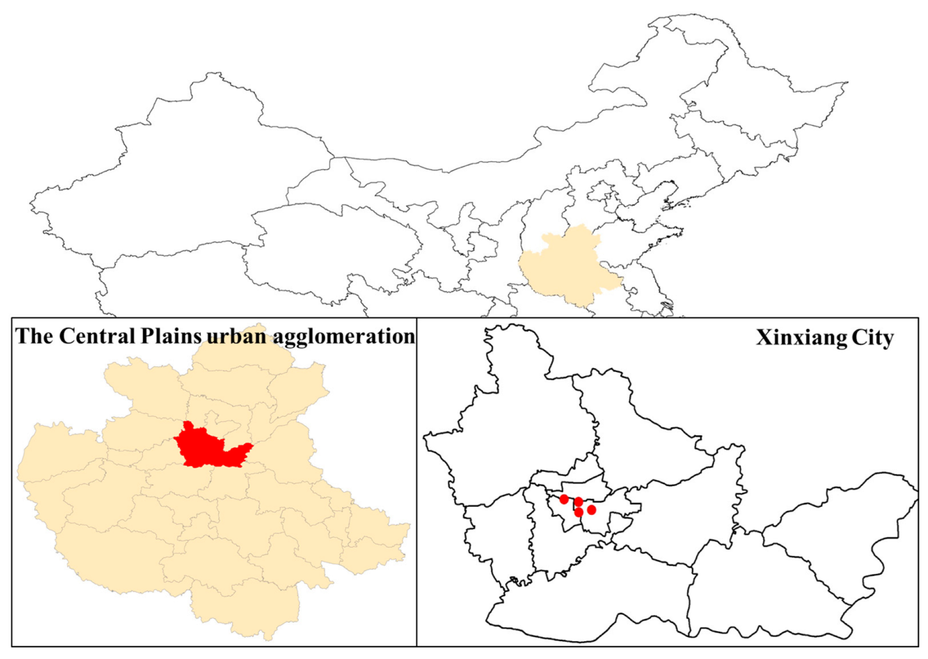
Xinxiang City has been equipped with four state-operated air quality automatic monitoring stations since 2015, which are strategically positioned primarily within the urban area (Figure 1). Hourly concentrations of air pollutants (including O3, NO2, CO, SO2, PM2.5, and PM10) from these four sites were obtained from the China National Environmental Monitoring Centre (http://www.cnemc.cn/, accessed on 16 May 2024), covering the period from 1 January 2015 to 31 December 2022. The pollutants data were normalized based on the change of atmospheric conditions before (273.15 K, 1 atm) and after (298.15 K, 1 atm) September 2018.
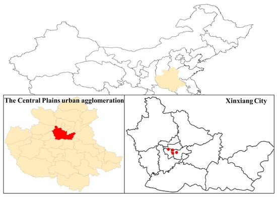
Figure 1.
Location of the nation-controlled air quality automatic monitoring stations in Xinxiang City. The red dots represent four state-operated air quality automatic monitoring stations.
The meteorological data from 1 January 2015 to 31 December 2022 were obtained from the ERA5 datasets of the European Centre for Medium-Range Weather Forecasts (ECMWF) (https://cds.climate.copernicus.eu/cdsapp#!/dataset/reanalysis-era5-single-levels?tab=overview, accessed on 19 May 2024). The research area (34°55′–35°50′ E; 113°30′–115°01′ N) covered the entire Xinxiang City. The hourly resolution of significant meteorological variables involving the O3 formation mechanism with a spatial resolution of 0.25° × 0.25° was utilized in our study, including a 10 m u-component of wind, 10 m v-component of wind, 2 m dewpoint temperature, 2 m temperature, boundary layer height, surface net solar radiation, surface pressure, total cloud cover, and total precipitation. The detailed information of these variables can be found in Table 1.

Table 1.
The main information of the nine meteorological variables.
The field measurement campaign was also conducted from 1 June to 31 June in 2021. The sampling site was located at the Xinxiang Municipal Party School (35.29° N, 113.93° E), a typical urban area. The gaseous pollutants, including O3, NO2, NO, SO2, CO, and NMVOCs, were measured in our study. The Model 42i, Model 48i, Model 43i, and Model 49i (Thermo Fisher Scientific, Waltham, MA, USA) were used for online measurements of NOx (NO2, NO), SO2, CO, and O3. The hourly NMVOCs concentrations, including alkanes, alkenes, alkynes, aromatics, and oxygenated compounds were measured by GC-FID/MS (TH-300B, Wuhan Tianhong Environmental Protection Industry Co., Ltd., Wuhan, China).
2.2. Random Forest Model
The RF model is an ensemble learning algorithm with high accuracy and a strong ability to avoid overfitting. Here, the RF model was developed to predict the concentrations of O3 and identify critical variables in O3 formation. The performance of RF depends on hyperparameters. Details of all parameters tuned for the RF model are presented in Table S1. The randomForest package for the R software (version 4.2.3) is used for analyses and validation processes in our study.
For the RF model, the in situ observation pollutants concentrations and meteorology factors were selected as input variables. Due to a lack of long-term hourly observation, VOCs were excluded from the input parameters in this study. According to previous studies [37,38,39,40], the variability of surface O3 was well-explained by the ML algorithm with meteorological information alone, particularly in the VOC-limited regime. Like many other urban areas in China, O3 production in Xinxiang City is generally in the VOC-limited regime. Therefore, it is reasonable to simulate O3 using a supervised RF model without considering the VOC concentration.
The datasets were randomly divided into training and testing subsets at a ratio of 7:3. The fivefold cross-validation method was used to evaluate the performance of the RF model [27] (Figure S1). The relative importance of the input variables was ranked by calculated variable importance scores, represented as the aggregated increase in the mean squared errors (%IncMSE). The mean squared errors were calculated by the RF model by randomly assigning values to each input variable. The variables with a higher importance score (%IncMSE) had a more significant impact on O3 formation.
2.3. Observation-Based Model
OBM incorporated with MCM v3.3.1 was built to investigate the chemical mechanism of how PM2.5 affects the formation of O3. The detailed description of the gas-phase chemical processes by the MCM displays that it was involved in methane and 142 non-methane VOCs [41]. To establish a direct relationship between PM2.5 concentrations and O3 formation, the OBM considered the heterogeneous reactions and variations in photolysis rates. The aerosol optical depth (AOD) could be calculated by the PM2.5 concentration [23,42] using Equation (1):
where H represents the atmosphere boundary layer height; f(RH) denotes the hygroscopic growth factor, which is determined by relative humidity (RH), and K is the given parameter.
The calculated AOD was used to quantify the hourly photolysis rates of NO2 (JNO2) [43,44], thus establishing a direct link between PM2.5 concentration and photolysis rates (see details in the Supplemental Information). The photolysis rates (Ji) of other species were calculated by the solar zenith angle (SZA) and built-in parameters (Li, Mi, and Ni) [45]; see Equation (2):
The photolysis rates would be further scaled according to the calculated photolysis rates of NO2 (JNO2) based on the PM2.5 concentration.
The heterogeneous reaction of HO2 was assumed to be the first order reaction [21,46], and the reaction constant (k) could be calculated by Equation (3):
where r, Dg, and vHO2 were the surface-weighted particle radius, gas phase diffusion coefficient, and mean molecular speed of HO2, respectively. The relevant values of these parameters were selected according our previous study [33]. γHO2 was the uptake coefficient of HO2 on aerosols, ranging from 0.02 to 0.2. The O3 concentration under different γHO2 was tested by OBM (Figure S1). In our study, the maximum γHO2 value of 0.2 was adopted to magnify the effect by the model according to Shao et al.’s study [23]. Saero was the aerosol surface concentration, which is calculated by the PM2.5 concentration (further details are provided in the Supplemental Information).
The observed and calculated data, including pollutant concentrations (CO, SO2, NOx (NO, NO2), and NMVOCs) and meteorological factors (relative humidity, temperature, pressure, and the photolysis rates in related species) were subjected to the model constraints. The time resolution of the input parameters was averaged or interpolated to 1 h.
2.4. Model Evaluation
The mean bias (MB), root mean squared error (RMSE), and index of agreement (IOA) were used to assess the model (RF and OBM) performance based on the observed (Oi) and simulated (Si) hourly O3 values according to the following equations:
where is the mean concentration of the observed O3.
3. Results and Discussion
3.1. O3 Pollution Profiles
3.1.1. Long-Term Trend of O3 and Related Pollutants
The year variations of 1 h O3 concentrations and related pollutants (NO2 and PM2.5) in Xinxiang City are presented in Figure 2. The O3 concentration exhibited an increasing trend from 2015 to 2022, with an average growth rate of 3.41 μg m−3 yr−1. The similar upward trends in O3 concentrations over the past 1–2 decades have been observed in other Chinese urban areas, such as Beijing [47], Shanghai [48], the Sichuan Basin [6], the Pearl River Delta [49], and various other Chinese urban sites [2,7]. In contrast, the concentrations of PM2.5 and NO2 showed significant declines from 2015 to 2022. This reduction is attributed to the stringent implementation of clean air policies in China, including the Air Pollution Prevention and Control Action Plan (2013–2017) and the Three-Year Action Plan for Winning the Blue Sky Defense Battle (2018–2020) [3]. The former plan focused primarily on reducing particulate matter, while the latter emphasized the coordinated control of NOx and VOCs, with a targeted 10% reduction in VOC emissions [50].
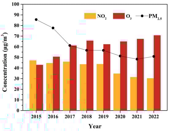
Figure 2.
The annual trend of O3, NO2, and PM2.5 during 2015–2022.
The increasing O3 trend could be further separated into two phases (Phase I, 2015–2018; Phase II, 2019–2022) based on the different increasing rate. During Phase I, the average 1-hourly O3 concentration increased at a rate of 7.89 μg m−3 yr−1. The average annual concentration of PM2.5 was at a high level, and had a significant decrease (from 85.54 to 56.70 μg m−3). However, no significant changes were observed in NO2 concentration during Phase I. In contrast, during Phase II, the increase rate of O3 was 2.76 μg m−3 yr−1, which was much smaller than that in Phase I. The concentration of PM2.5 was also at the high level (approximately 50 μg m−3), although it experienced a relatively smaller decrease compared to Phase I. By contrast, the concentration of NO2 had an obvious decreasing tendency in Phase II.
NO2 was the important precursor in O3 formation through the “NOx cycle”, exhibiting a non-linear relationship with O3 formation. Under the VOC-limited conditions, which were thought to prevail in urban China, decreasing NOx would increase O3, while under NOx-limited conditions, reducing NOx could decrease O3 concentrations [22]. The effect of PM2.5 on O3 formation was mainly by changing photolysis rates and heterogeneous chemical processes [23], with its influence heavily dependent on the level of the PM2.5 concentration. In Xinxiang City, O3 formation was under VOC-limited regimes alongside a high PM2.5 concentration. In the condition, reductions in both NOx and PM2.5 can lead to increased O3 production. Hence, the decline in PM2.5 concentration could be a primary factor driving the rise in O3 in Phase I. The result was consistent with the results that a reduction of PM2.5 stimulated O3 production over the 2013–2017 periods in the North China Plain. The impact of PM2.5 controls on O3 formation likely weakened in Phase II due to the relatively minor reduction in PM2.5 concentrations. The unbalanced changing of the precursor concentration (VOC and NO2) might be the main reason for O3 increasing in Phase II.
3.1.2. Seasonal Variation of O3 Pollution
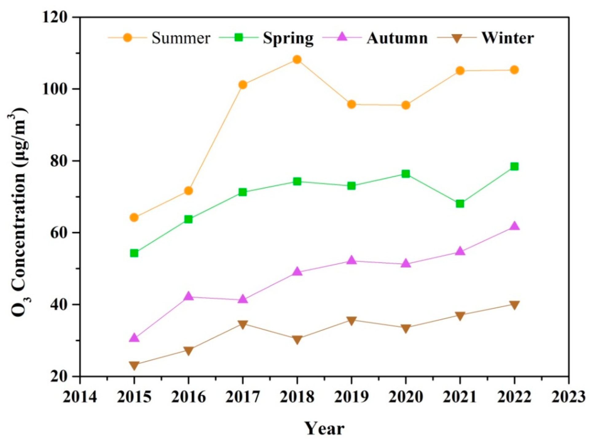
The seasonal variation of O3 during 2015–2022 is shown in Figure 3. O3 concentrations exhibit pronounced seasonal patterns, peaking during the summer, and remaining at relatively lower levels in the winter. The rise in temperature and solar radiation intensity plays a critical role in photochemical formation of O3 in summer [51]. Enhanced photochemical production and the rapid cycling of ROx radicals (OH + HO2 + RO + RO2) typically overcome the radical and NO titration in summer [52]. Consequently, the potential health hazards associated with O3 exposure are particularly significant during the warm season. According to the updated WHO Global Air Quality Guidelines (AQGs) from September 2021, the recommended peak season O3 concentration is lower than 60 μg m−3. However, the average concentration of O3 in summer and spring exceed the recommended threshold from 2015 to 2022. In autumn and winter, a steady increase in O3 concentration has been observed since 2018, with levels exceeding 60 μg m−3 in autumn 2022. The extension of the O3 pollution season from the warm season is a nationwide phenomenon in China [53]. The rapid rise in O3 levels outside of the summer season can enhance atmospheric oxidative capacity, potentially leading to the increased formation of secondary PM2.5, including nitrate, sulfate, and organic components.
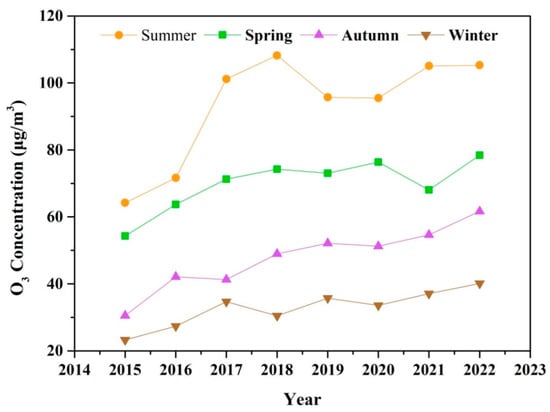
Figure 3.
The seasonal variation of O3 pollution during 2015–2022.
3.2. Identifying Key Factors Using RF Models
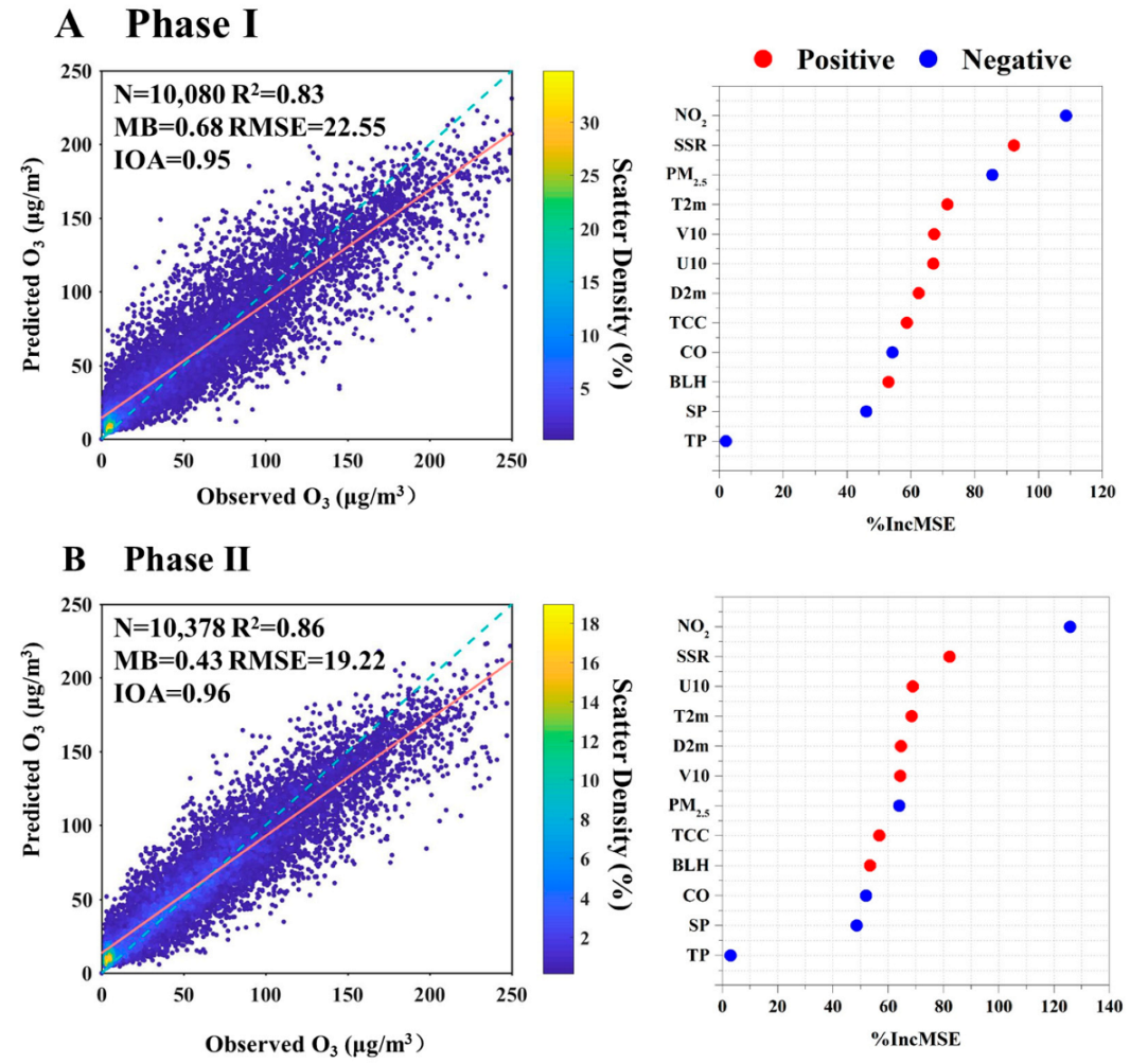
The RF model was employed to predict O3 concentrations for both Phase I and Phase II. As shown in Figure S3, during the training phase, the model explained 83% and 86% of the measured O3 for Phase I and Phase II, respectively. The RMSE was 9.55 and 7.96 μg m−3 for Phase I and Phase II, respectively. The performances of the testing dataset in RF model for the two phases are shown in Figure 4. For both phases, the values of MB were minor, and the values of R2 and IOA were close to 1. The slope and intercept values were 0.77 and 14.25 for Phase I and 0.79 and 13.49 for Phase II. It is noteworthy that the RF model tended to underestimate and overestimate O3 concentrations at relatively high and low values, resulting in relatively higher RMSE for both phases. This discrepancy can be attributed to the RF model’s tendency to exhibit larger biases in predicting extreme values due to the absence of certain O3 precursor data, such as VOC [29,54]. Nevertheless, the RF model could successful reproduce O3 concentration using the selected factors.

Figure 4.
Model performance and variable importance for two phases: (A) Phase I, (B) Phase II. Cross-validated models R2 and MB, RMSE, and IOA are calculated by using a fivefold cross-validation modeling performance for 1 h O3 concentration. The orange line and blue dotted line represent the fitted and 1:1 line. The variables are listed in the order of importance from top to bottom. The horizontal axis represents the aggregated increase in the mean squared errors (%IncMSE) from the RF model. A larger value represents higher importance. The correlation relationships (positive and negative) of O3 with the variables are identified.
As shown in Figure 4, the top 5 factors for Phase I were NO2, SSR, PM2.5, T2m, and V10. The photolysis of NO2 produced an oxygen atom, and O3 was then produced from the combination of the oxygen atom and O2 [1]. Hence, NO2 and SSR were the notably influential factors in O3 formation. PM2.5 was identified as the third most significant factor contributing to O3 formation in Phase I. The reduction of PM2.5 during this phase may elevate O3 concentrations through modulations in atmospheric heterogeneous reaction kinetics, solar radiation-driven photolysis efficiencies, and planetary boundary layer transport dynamics [20,22]. Temperature was also an important factor influencing O3 formation in Phase I. Chemical kinetics rates involved in O3 production increased with the increase of temperature [55]. Additionally, the VOC emissions, including biogenic emission rates and anthropogenic emissions (such as solvent evaporation), may be enhanced in hot weather [56,57].
In Phase II, NO2 and SSR remained prominent factors, indicating the local formation of O3. Other high-ranking variables were predominantly meteorology-related, including U10, D2m, T2m, and V10. Unlike in Phase I, PM2.5 was less important due to the relatively smaller change in the concentrations in Phase II. O3 enhancement due to PM2.5 dropping significantly depends on the current level of PM2.5 concentration and its decline magnitude [22,23]. The decreased amplitude and the level of PM2.5 concentrations were smaller in Phase II, resulting in less importance of PM2.5 in O3 formation. Although PM2.5 ranked seventh in Phase II, its %IncMSE value was close to the high-ranking meteorology-related factors—higher than BLH and CO. In addition, the concentration of PM2.5 was at a high level (about 51 μg m−3 in 2022), exceeding Class I limit values of the National Ambient Air Quality Standard (NAAQS) (35 μg m−3). Hence, PM2.5 remains a significant factor in O3 formation in recent years for Xinxiang City and also for the other cities with a high PM2.5 concentration.
3.3. Role of PM2.5 in O3 Formation
From 19 June to 25 June 2021, the average O3 concentration (128.63 μg m−3) was in excess of the CNAAQS 1 h mass-based standards of 120 μg m−3. The period was identified as being traceable to an O3 episode. During the episode, a high level of O3 concentration (up to 257 μg m−3) was observed. The concentrations of SO2, NO, NO2, and CO were 13.60, 3.64, 32.46 μg m−3, and 0.50 mg m−3 on average. The PM2.5 concentration was at a relatively low level, with 25.00 μg m−3 being the average. The average mixing ratios of 35 NMVOCs are summarized in Table S2. The other information about the O3 episode is also introduced in the Supplementary Materials.
The identified O3 episode (19 June to 25 June 2021) was used by OBM for a simulation study. The comparison of observed and simulated O3 during the identified O3 episode is shown in Figure S4. The model accurately captured the diurnal profile of O3, demonstrating satisfactory performance. The average concentration of observed and simulated O3 during the episode was 128.09 and 128.63 μg m−3, respectively, with a high R2 value of 0.96. In addition, the MB, RMSE, and IOA were 0.82 μg m−3, 8.08 μg m−3, and 0.97, respectively, further validating the model’s capability to reproduce the variations of O3 effectively and enabling its use for subsequent analysis.
As mentioned in Section 2.3, the heterogeneous reactions and changing of photolysis rates linked to PM2.5 were incorporated into the model. Hence, we conducted experiments to assess how variations in PM2.5 concentration affected O3 levels. During the episode, the concentration of PM2.5 was relatively low, with about 25 μg m−3 on average. To illustrate concrete situations of pollution, O3 concentration was simulated by OBM with a series of PM2.5 concentrations (0–3 times PM2.5 concentration). The diurnal profile of O3 concentration under different PM2.5 concentrations is shown in Figure S5. The O3 concentration rose with the dropping of the PM2.5 concentration. The maximum disparity in O3 concentration under different PM2.5 concentrations reached up to 32.46 μg m−3 (Figure S6), indicating the significant impact of PM2.5 on O3 formation. In addition, the rangeabilities of O3 under difference PM2.5 concentrations was higher in the daytime and lower at nighttime. The reduction of HO2 by heterogeneous loss in PM2.5 was the major mechanism at nighttime. The decrease in PM2.5 could lead to an increasing HO2 concentration due to less HO2 heterogeneous loss on the ambient aerosol [22]. The NO titration effect on O3 could be offset by an elevated HO2 concentration [11]. During the daytime, enhanced photolysis rates resulting from decreased PM2.5 concentration further facilitated O3 formation. Both mechanisms played significant roles in O3 formation during the daytime.
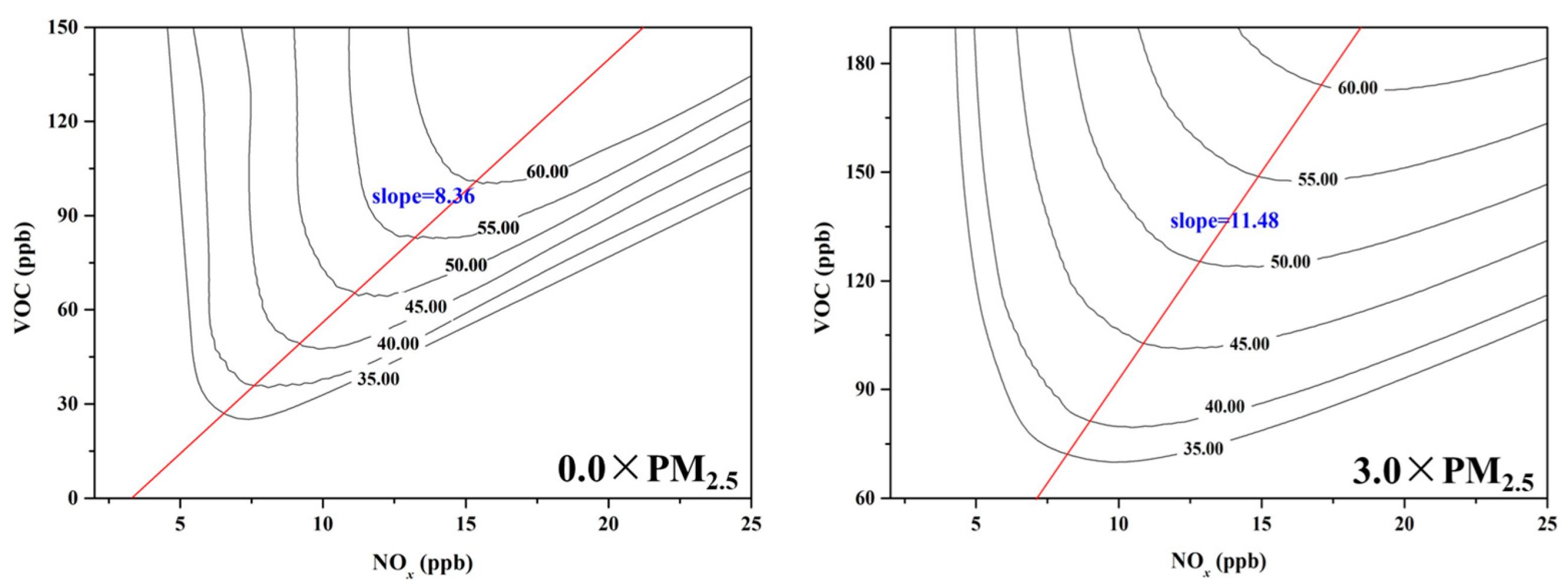
The Empirical Kinetic Modeling Approach (EKMA) diagram can categorize O3 formation into either “NOx limited” or “VOC limited” regime [20], providing a basis for effective O3 pollution control policies. To investigate the impact of PM2.5 on O3 pollution control strategies, EKMA curves were constructed by OBM under both 0.0 × PM2.5 and 3.0 × PM2.5 scenarios (Figure 5). The EKMA curve was changed under different concentrations of PM2.5, with the slope of the ridgeline (VOC/NOx) increasing from 8.36 under 0.0 × PM2.5 scenarios to 11.48 under 3.0 × PM2.5 scenarios. The result meant that the O3 formation regime tended to “NOx limited” with the dropping of PM2.5 concentration. PM2.5 has a great impact on the O3 sensitivity regime, thereby affecting the production rate of surface O3. The aerosol chemistry and photochemistry were the main mechanism for the shift of O3 chemical regimes under different PM2.5 concentrations [58]. As previously discussed, the concentration of the HO2 concentration increases as the level of PM2.5 declines, accelerating the ROx cycle (OH→RO→RO2→HO2→OH) with peroxyl-radical self-reactions predominating under these conditions. Therefore, when formulating policies for VOC and NOx emission reductions to control O3 pollution, it is crucial to pay more attention to changes in PM2.5 concentration [44].
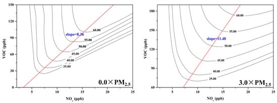
Figure 5.
The EKMA under different PM2.5 concentrations.
3.4. Limitations
In the present study, a comprehensive dataset from field measurements was employed as a model constraint. The dataset included key parameters, such as the concentrations of reactive species, mixing layer height, and photolysis frequencies. Additionally, the state-of-the-art gas chemistry mechanism (MCM) was used in the OBM. The uncertainties of the OBM were mainly determined by the complexities of atmospheric “Haze Chemistry” [59]. Multiple heterogeneous reactions coexisted on the aerosol surfaces [60,61]. Therefore, some heterogeneous reaction might have an impact on O3 production, such as the heterogeneous formation of HONO and HNO3 [62] and heterogeneous loss of O3 [63]. However, the heterogeneous reactions mechanism was unrevealed, with a big range of heterogeneous uptake coefficients [11,22]. Hence, only the heterogeneous reaction of HO2 on aerosols surfaces, the paramount heterogeneous reaction impacting O3 formation, was considered in our study.
4. Conclusions
Clean air actions have been implemented by the Chinese government to improve the severe air pollution issue since 2013. However, the increasing trend of O3 has been inconsistent with the decline of PM2.5 in China. In Xinxiang City, the O3 concentration increased by the rate of 3.41 μg m−3 yr−1 from 2015 to 2022. This increase can be divided into two phases: Phase I (2015–2018) saw a high rate of increase (7.89 μg m−3), while Phase II (2019–2022) experienced a lower rate (2.89 μg m−3). The O3 pollution from warm seasons should be paid more attention, due to the steady increasing O3 concentration in autumn and winter since 2018. The developed RF model effectively simulated O3 concentrations, identifying NO2 and surface net solar radiation as primary factors in O3 formation for both phases. In Phase I, PM2.5 ranked third in O3 formation, while in Phase II, PM2.5 remained a significant factor due to its persistently high concentration in Xinxiang City. The OBM incorporated into MCM was used to explore how PM2.5 influences O3 formation. The O3 concentration was raised with the dropping of PM2.5 by the process of the heterogeneous reaction and photolysis rates. The O3 formation regime tended to “NOx limited” with the dropping of the PM2.5 concentration. Neglecting the role of PM2.5 in O3 formation could have adverse effects on O3 pollution control policies. Further research into heterogeneous uptake coefficients would be beneficial in reducing the uncertainties associated with heterogeneous reactions in real atmospheric aerosols. Our results provide powerful evidence for on-going coordinated control of O3 and PM2.5 in a typical city of the Central Plains urban agglomeration.
Supplementary Materials
The following supporting information can be downloaded at: https://www.mdpi.com/article/10.3390/toxics13050330/s1, Text S1: Details setting in OBM; Figure S1: The error rate curve of RF model by fivefold cross-validation method; Figure S2: The simulated O3 concentrations with different uptake coefficient of HO2 (γHO2) on aerosols; Figure S3: The performances of the training dataset in RF model for Phase I and Phase II; Figure S4: The comparison of simulated and observed O3 concentrations; Figure S5: The diurnal profile of O3 under a series of PM2.5 concentrations; Figure S6: The simulated maximum O3 concentration by OBM under different PM2.5 concentrations; Table S1: Parameters tuned for RF model; Table S2: The average concentration of VOC during the sampling period.
Author Contributions
C.J.: Conceptualization, Methodology, Software, Formal analysis, Writing—Original Draft, G.Y.: Investigation, Validation, Writing—Reviewing and Editing, X.Y.: Investigation, Data Curation, X.L.: Investigation, Data Curation, J.X.: Investigation, Data Curation, Y.W.: Conceptualization, Methodology, Writing—Reviewing and Editing, Z.C.: Supervision, Writing—Reviewing and Editing, Funding acquisition. All authors have read and agreed to the published version of the manuscript.
Funding
This research was funded by the Scientific Research Foundation of Henan Normal University (NO. 5101219170837), Xinxiang Major Science and Technology Plan Project (NO. 22ZD002), and the National Natural Science Foundation of China (NO. 41977308).
Institutional Review Board Statement
Not applicable.
Informed Consent Statement
Not applicable.
Data Availability Statement
The data that support the findings of this study are available from the corresponding author upon reasonable request.
Conflicts of Interest
The authors declare no conflicts of interest.
References
- Lyu, X.; Li, K.; Guo, H.; Morawska, L.; Zhou, B.; Zeren, Y.; Jiang, F.; Chen, C.; Goldstein, A.H.; Xu, X.; et al. A synergistic ozone-climate control to address emerging ozone pollution challenges. One Earth 2023, 6, 964–977. [Google Scholar] [CrossRef]
- Liu, Y.; Geng, G.; Cheng, J.; Liu, Y.; Xiao, Q.; Liu, L.; Shi, Q.; Tong, D.; He, K.; Zhang, Q. Drivers of Increasing Ozone during the Two Phases of Clean Air Actions in China 2013–2020. Environ. Sci. Technol. 2023, 57, 8954–8964. [Google Scholar] [CrossRef] [PubMed]
- Wang, W.; Parrish, D.D.; Wang, S.; Bao, F.; Ni, R.; Li, X.; Yang, S.; Wang, H.; Cheng, Y.; Su, H. Long-term trend of ozone pollution in China during 2014–2020: Distinct seasonal and spatial characteristics and ozone sensitivity. Atmos. Chem. Phys. 2022, 22, 8935–8949. [Google Scholar] [CrossRef]
- Zhang, L.; Wang, L.L.; Liu, B.Y.; Tang, G.Q.; Liu, B.X.; Li, X.; Sun, Y.; Li, M.G.; Chen, X.Y.; Wang, Y.S.; et al. Contrasting effects of clean air actions on surface ozone concentrations in different regions over Beijing from May to September 2013–2020. Sci. Total Environ. 2023, 903, 166182. [Google Scholar] [CrossRef]
- Qian, J.; Liao, H.; Yang, Y.; Li, K.; Chen, L.; Zhu, J. Meteorological influences on daily variation and trend of summertime surface ozone over years of 2015-2020: Quantification for cities in the Yangtze River Delta. Sci. Total Environ. 2022, 834, 155107. [Google Scholar] [CrossRef]
- Wu, K.; Wang, Y.R.; Qiao, Y.H.; Liu, Y.M.; Wang, S.G.; Yang, X.Y.; Wang, H.L.; Lu, Y.Q.; Zhang, X.L.; Lei, Y. Drivers of 2013–2020 ozone trends in the Sichuan Basin, China: Impacts of meteorology and precursor emission changes. Environ. Pollut. 2022, 300, 118914. [Google Scholar] [CrossRef]
- Lu, X.; Zhang, L.; Wang, X.L.; Gao, M.; Li, K.; Zhang, Y.Z.; Yue, X.; Zhang, Y.H. Rapid Increases in Warm-Season Surface Ozone and Resulting Health Impact in China Since 2013. Environ. Sci. Technol. Lett. 2020, 7, 240–247. [Google Scholar] [CrossRef]
- Chen, X.; Jiang, Z.; Shen, Y.; Li, R.; Fu, Y.; Liu, J.; Han, H.; Liao, H.; Cheng, X.; Jones, D.B.A.; et al. Chinese Regulations Are Working—Why Is Surface Ozone Over Industrialized Areas Still High? Applying Lessons From Northeast US Air Quality Evolution. Geophys. Res. Lett. 2021, 48, e2021GL092816. [Google Scholar] [CrossRef]
- Li, K.; Jacob, D.J.; Shen, L.; Lu, X.; Smedt, I.D.; Liao, H.; PHYSICS. Increases in surface ozone pollution in China from 2013 to 2019: Anthropogenic and meteorological influences. Atmos. Chem. Phys. 2020, 20, 11423–11433. [Google Scholar] [CrossRef]
- Wang, T.; Xue, L.K.; Brimblecombe, P.; Lam, Y.F.; Li, L.; Zhang, L. Ozone pollution in China: A review of concentrations, meteorological influences, chemical precursors, and effects. Sci. Total Environ. 2017, 575, 1582–1596. [Google Scholar] [CrossRef]
- Tan, Z.; Hofzumahaus, A.; Lu, K.; Brown, S.S.; Holland, F.; Huey, L.G.; Kiendler-Scharr, A.; Li, X.; Liu, X.; Ma, N.; et al. No Evidence for a Significant Impact of Heterogeneous Chemistry on Radical Concentrations in the North China Plain in Summer 2014. Environ. Sci. Technol. 2020, 54, 5973–5979. [Google Scholar] [CrossRef]
- Li, M.; Wang, T.; Shu, L.; Qu, Y.; Xie, M.; Liu, J.; Wu, H.; Kalsoom, U. Rising surface ozone in China from 2013 to 2017: A response to the recent atmospheric warming or pollutant controls? Atmos. Environ. 2021, 246, 118130. [Google Scholar] [CrossRef]
- Ding, J.; Dai, Q.; Fan, W.; Lu, M.; Zhang, Y.; Han, S.; Feng, Y. Impacts of meteorology and precursor emission change on O3 variation in Tianjin, China from 2015 to 2021. J. Environ. Sci. 2023, 126, 506–516. [Google Scholar] [CrossRef] [PubMed]
- Xiong, K.; Xie, X.; Mao, J.; Wang, K.; Huang, L.; Li, J.; Hu, J. Improving the accuracy of O3 prediction from a chemical transport model with a random forest model in the Yangtze River Delta region, China. Environ. Pollut. 2023, 319, 120926. [Google Scholar] [CrossRef] [PubMed]
- Li, L.; Xie, F.; Li, J.; Gong, K.; Xie, X.; Qin, Y.; Qin, M.; Hu, J. Diagnostic analysis of regional ozone pollution in Yangtze River Delta, China: A case study in summer 2020. Sci. Total Environ. 2022, 812, 151511. [Google Scholar] [CrossRef] [PubMed]
- Shi, Z.; Huang, L.; Li, J.; Ying, Q.; Hu, J. Sensitivity analysis of the surface ozone and fine particulate matter to meteorological parameters in China. Atmos. Chem. Phys. 2020, 20, 13455–13466. [Google Scholar] [CrossRef]
- Qin, Y.; Li, J.; Gong, K.; Wu, Z.; Chen, M.; Qin, M.; Huang, L.; Hu, J. Double high pollution events in the Yangtze River Delta from 2015 to 2019: Characteristics, trends, and meteorological situations. Sci. Total Environ. 2021, 792, 148349. [Google Scholar] [CrossRef]
- Weng, X.; Forster, G.L.; Nowack, P. A machine learning approach to quantify meteorological drivers of ozone pollution in China from 2015 to 2019. Atmos. Chem. Phys. 2022, 22, 8385–8402. [Google Scholar] [CrossRef]
- Tan, Z.; Lu, K.; Ma, X.; Chen, S.; He, L.; Huang, X.; Li, X.; Lin, X.; Tang, M.; Yu, D.; et al. Multiple Impacts of Aerosols on O3 Production Are Largely Compensated: A Case Study Shenzhen, China. Environ. Sci. Technol. 2022, 56, 17569–17580. [Google Scholar] [CrossRef]
- Ivatt, P.D.; Evans, M.J.; Lewis, A.C. Suppression of surface ozone by an aerosol-inhibited photochemical ozone regime. Nat. Geosci. 2022, 15, 536–540. [Google Scholar] [CrossRef]
- Dyson, J.E.; Whalley, L.K.; Slater, E.J.; Woodward-Massey, R.; Ye, C.X.; Lee, J.D.; Squires, F.; Hopkins, J.R.; Dunmore, R.E.; Shaw, M.; et al. Impact of HO2 aerosol uptake on radical levels and O3 production during summertime in Beijing. Atmos. Chem. Phys. 2023, 23, 5679–5697. [Google Scholar] [CrossRef]
- Li, K.; Jacob, D.J.; Liao, H.; Shen, L.; Zhang, Q.; Bates, K.H. Anthropogenic drivers of 2013–2017 trends in summer surface ozone in China. Proc. Natl. Acad. Sci. USA 2019, 116, 422–427. [Google Scholar] [CrossRef]
- Shao, M.; Wang, W.; Yuan, B.; Parrish, D.D.; Li, X.; Lu, K.; Wu, L.; Wang, X.; Mo, Z.; Yang, S.; et al. Quantifying the role of PM2.5 dropping in variations of ground-level ozone: Inter-comparison between Beijing and Los Angeles. Sci. Total Environ. 2021, 788, 147712. [Google Scholar] [CrossRef] [PubMed]
- Hou, L.; Dai, Q.; Song, C.; Liu, B.; Guo, F.; Dai, T.; Li, L.; Liu, B.; Bi, X.; Zhang, Y.; et al. Revealing Drivers of Haze Pollution by Explainable Machine Learning. Environ. Sci. Technol. Lett. 2022, 9, 112–119. [Google Scholar] [CrossRef]
- Vu, T.V.; Shi, Z.; Cheng, J.; Zhang, Q.; He, K.; Wang, S.; Harrison, R.M. Assessing the impact of clean air action on air quality trends in Beijing using a machine learning technique. Atmos. Chem. Phys. 2019, 19, 11303–11314. [Google Scholar] [CrossRef]
- Wang, L.; Zhao, Y.; Shi, J.; Ma, J.; Liu, X.; Han, D.; Gao, H.; Huang, T. Predicting ozone formation in petrochemical industrialized Lanzhou city by interpretable ensemble machine learning. Environ. Pollut. 2023, 318, 120798. [Google Scholar] [CrossRef] [PubMed]
- Watson, G.L.; Telesca, D.; Reid, C.E.; Pfister, G.G.; Jerrett, M. Machine learning models accurately predict ozone exposure during wildfire events. Environ. Pollut. 2019, 254, 112792. [Google Scholar] [CrossRef]
- Ma, R.; Ban, J.; Wang, Q.; Zhang, Y.; Yang, Y.; He, M.Z.; Li, S.; Shi, W.; Li, T. Random forest model based fine scale spatiotemporal O3 trends in the Beijing-Tianjin-Hebei region in China, 2010 to 2017. Environ. Pollut. 2021, 276, 116635. [Google Scholar] [CrossRef] [PubMed]
- Yang, J.; Wen, Y.; Wang, Y.; Zhang, S.; Pinto, J.P.; Pennington, E.A.; Wang, Z.; Wu, Y.; Sander, S.P.; Jiang, J.H.; et al. From COVID-19 to future electrification: Assessing traffic impacts on air quality by a machine-learning model. Proc. Natl. Acad. Sci. USA 2021, 118, e2102705118. [Google Scholar] [CrossRef]
- Zhan, J.; Liu, Y.; Ma, W.; Zhang, X.; Wang, X.; Bi, F.; Zhang, Y.; Wu, Z.; Li, H. Ozone formation sensitivity study using machine learning coupled with the reactivity of volatile organic compound species. Atmos. Meas. Tech. 2022, 15, 1511–1520. [Google Scholar] [CrossRef]
- Zhu, J.; Wang, S.; Wang, H.; Jing, S.; Lou, S.; Saiz-Lopez, A.; Zhou, B. Observationally constrained modeling of atmospheric oxidation capacity and photochemical reactivity in Shanghai, China. Atmos. Chem. Phys. 2020, 20, 1217–1232. [Google Scholar] [CrossRef]
- Edwards, P.M.; Brown, S.S.; Roberts, J.M.; Ahmadov, R.; Banta, R.M.; deGouw, J.A.; Dubé, W.P.; Field, R.A.; Flynn, J.H.; Gilman, J.B.; et al. High winter ozone pollution from carbonyl photolysis in an oil and gas basin. Nature 2014, 514, 351–354. [Google Scholar] [CrossRef] [PubMed]
- Jia, C.; Tong, S.; Zhang, X.; Li, F.; Zhang, W.; Li, W.; Wang, Z.; Zhang, G.; Tang, G.; Liu, Z.; et al. Atmospheric oxidizing capacity in autumn Beijing: Analysis of the O3 and PM2.5 episodes based on observation-based model. J. Environ. Sci. 2023, 124, 557–569. [Google Scholar] [CrossRef]
- Michoud, V.; Kukui, A.; Camredon, M.; Colomb, A.; Borbon, A.; Miet, K.; Aumont, B.; Beekmann, M.; Durand-Jolibois, R.; Perrier, S.; et al. Radical budget analysis in a suburban European site during the MEGAPOLI summer field campaign. Atmos. Chem. Phys. 2012, 12, 11951–11974. [Google Scholar] [CrossRef]
- Li, Z.; Xue, L.; Yang, X.; Zha, Q.; Tham, Y.J.; Yan, C.; Louie, P.K.K.; Luk, C.W.Y.; Wang, T.; Wang, W. Oxidizing capacity of the rural atmosphere in Hong Kong, Southern China. Sci. Total Environ. 2018, 612, 1114–1122. [Google Scholar] [CrossRef]
- Ling, Z.H.; Guo, H.; Lam, S.H.M.; Saunders, S.M.; Wang, T. Atmospheric photochemical reactivity and ozone production at two sites in Hong Kong: Application of a Master Chemical Mechanism–photochemical box model. J. Geophys. Res.-Atmos. 2015, 119, 10567–10582. [Google Scholar] [CrossRef]
- Balamurugan, V.; Balamurugan, V.; Chen, J. Importance of ozone precursors information in modelling urban surface ozone variability using machine learning algorithm. Sci. Rep. 2022, 12, 5646. [Google Scholar] [CrossRef]
- Gong, X.; Hong, S.; Jaffe, D.A. Ozone in China: Spatial Distribution and Leading Meteorological Factors Controlling O3 in 16 Chinese Cities. Aerosol Air Qual. Res. 2018, 18, 1–14. [Google Scholar] [CrossRef]
- Hu, C.; Kang, P.; Jaffe, D.A.; Li, C.; Zhou, M. Understanding the impact of meteorology on ozone in 334 cities of China. Atmos. Environ. 2021, 248, 118221. [Google Scholar] [CrossRef]
- Brancher, M. Increased ozone pollution alongside reduced nitrogen dioxide concentrations during Vienna’s first COVID-19 lockdown: Significance for air quality management. Environ. Pollut. 2021, 284, 117153. [Google Scholar] [CrossRef]
- Jenkin, M.E.; Young, J.C.; Rickard, A.R. The MCM v3.3.1 degradation scheme for isoprene. Atmos. Chem. Phys. 2015, 15, 11433–11459. [Google Scholar] [CrossRef]
- Lin, C.; Li, Y.; Yuan, Z.; Lau, A.K.H.; Li, C.; Fung, J.C.H. Using satellite remote sensing data to estimate the high-resolution distribution of ground-level PM2.5. Remote Sens. Environ. 2015, 156, 117–128. [Google Scholar] [CrossRef]
- Zhao, S.; Hu, B.; Du, C.; Liu, H.; Wang, Y. Photolysis rate in the Beijing-Tianjin-Hebei region: Reconstruction and long-term trend. Atmos. Res. 2021, 256, 105568. [Google Scholar] [CrossRef]
- Zhao, S.; Hu, B.; Liu, H.; Du, C.; Wang, Y. The influence of aerosols on the NO2 photolysis rate in a suburban site in North China. Sci. Total Environ. 2021, 767, 144788. [Google Scholar] [CrossRef]
- Jenkin, M.E.; Saunders, S.M.; Wagner, V.; Pilling, M.J. Protocol for the development of the Master Chemical Mechanism, MCM v3 (Part A): Tropospheric degradation of non-aromatic volatile organic compounds. Atmos. Chem. Phys. 2003, 3, 181–193. [Google Scholar] [CrossRef]
- Xue, L.K.; Wang, T.; Gao, J.; Ding, A.J.; Zhou, X.H.; Blake, D.R.; Wang, X.F.; Saunders, S.M.; Fan, S.J.; Zuo, H.C. Ground-level ozone in four Chinese cities: Precursors, regional transport and heterogeneous processes. Atmos. Chem. Phys. 2014, 14, 13175–13188. [Google Scholar] [CrossRef]
- Wang, W.; Parrish, D.; Li, X.; Shao, M.; Liu, Y.; Mo, Z.; Lu, S.; Hu, M.; Fang, X.; Wu, Y.; et al. Exploring the drivers of the increased ozone production in Beijing in summertime during 2005–2016. Atmos. Chem. Phys. 2020, 20, 15617–15633. [Google Scholar] [CrossRef]
- Gao, W.; Tie, X.X.; Xu, J.M.; Huang, R.J.; Mao, X.Q.; Zhou, G.Q.; Chang, L.Y. Long-term trend of O3 in a mega City (Shanghai), China: Characteristics, causes, and interactions with precursors. Sci. Total Environ. 2017, 603–604, 425–433. [Google Scholar] [CrossRef]
- Li, X.B.; Yuan, B.; Parrish, D.D.; Chen, D.H.; Song, Y.X.; Yang, S.X.; Liu, Z.J.; Shao, M. Long-term trend of ozone in southern China reveals future mitigation strategy for air pollution. Atmos. Environ. 2022, 269, 118869. [Google Scholar] [CrossRef]
- Li, K.; Jacob, D.; Liao, H.; Zhu, J.; Shah, V.; Shen, L.; Bates, K.; Zhang, Q.; Zhai, S. A two-pollutant strategy for improving ozone and particulate air quality in China. Nat. Geosci. 2019, 12, 906–910. [Google Scholar] [CrossRef]
- Ma, Z.; Xu, J.; Quan, W.; Zhang, Z.; Lin, W.; Xu, X. Significant increase of surface ozone at a rural site, north of eastern China. Atmos. Chem. Phys. 2016, 16, 3969–3977. [Google Scholar] [CrossRef]
- Jia, C.; Wang, Y.; Li, Y.; Huang, T.; Mao, X.; Mo, J.; Li, J.; Wanyanhan, J.; Liang, X.; Gao, H. Oxidative Capacity and Radical Chemistry in a Semi-arid and Petrochemical-industrialized City, Northwest China. Aerosol Air Qual. Res. 2018, 18, 1391–1404. [Google Scholar] [CrossRef]
- Li, K.; Jacob, D.J.; Liao, H.; Qiu, Y.; Shen, L.; Zhai, S.; Bates, K.H.; Sulprizio, M.P.; Song, S.; Lu, X.; et al. Ozone pollution in the North China Plain spreading into the late-winter haze season. Proc. Natl. Acad. Sci. USA 2021, 118, e2015797118. [Google Scholar] [CrossRef] [PubMed]
- Robinson, M.C.; Glen, R.C.; Lee, A.A. Validating the validation: Reanalyzing a large-scale comparison of deep learning and machine learning models for bioactivity prediction. J. Comput. Aid. Mol. Des. 2020, 34, 717–730. [Google Scholar] [CrossRef]
- Bloomer, B.J.; Stehr, J.W.; Piety, C.A.; Salawitch, R.J.; Dickerson, R.R. Observed relationships of ozone air pollution with temperature and emissions. Geophys. Res. Lett. 2009, 36, 269–277. [Google Scholar] [CrossRef]
- Gao, M.; Wang, F.; Ding, Y.H.; Wu, Z.W.; Xu, Y.Y.; Lu, X.; Wang, Z.F.; Carmichael, G.R.; McElroy, M.B. Large-scale climate patterns offer preseasonal hints on the co- occurrence of heat wave and O3 pollution in China. Proc. Natl. Acad. Sci. USA 2023, 120, e2218274120. [Google Scholar] [CrossRef]
- Wang, H.L.; Wu, K.; Liu, Y.M.; Sheng, B.S.; Lu, X.; He, Y.P.; Xie, J.L.; Wang, H.C.; Fan, S.J. Role of Heat Wave-Induced Biogenic VOC Enhancements in Persistent Ozone Episodes Formation in Pearl River Delta. J. Geophys. Res.-Atmos. 2021, 126, e2020JD034317. [Google Scholar] [CrossRef]
- Liu, C.; Liang, J.; Li, Y.; Shi, K. Fractal analysis of impact of PM2.5 on surface O3 sensitivity regime based on field observations. Sci. Total Environ. 2023, 858, 160136. [Google Scholar] [CrossRef]
- Biwu, C.; Qingxin, M.; Fengkui, D.; Jinzhu, M.; Jingkun, J.; Kebin, H.; Hong, H. Atmospheric “Haze Chemistry”: Concept and Research Prospects. Prog. Chem. 2020, 32, 1–4. [Google Scholar]
- Jacob, D.J. Heterogeneous chemistry and tropospheric ozone. Atmos. Environ. 2000, 34, 2131–2159. [Google Scholar] [CrossRef]
- Liu, Y.; He, G.; Chu, B.; Ma, Q.; He, H. Atmospheric heterogeneous reactions on soot: A review. Fundam. Res. 2023, 3, 579–591. [Google Scholar] [CrossRef] [PubMed]
- Li, Q.Y.; Zhang, L.; Wang, T.; Wang, Z.; Fu, X.; Zhang, Q. “New” Reactive Nitrogen Chemistry Reshapes the Relationship of Ozone to Its Precursors. Environ. Sci. Technol. 2018, 52, 2810–2818. [Google Scholar] [CrossRef] [PubMed]
- Kamm, S.; Möhler, O.; Naumann, K.H.; Saathoff, H.; Schurath, U. The heterogeneous reaction of ozone with soot aerosol. Atmos. Environ. 1999, 33, 4651–4661. [Google Scholar] [CrossRef]

Disclaimer/Publisher’s Note: The statements, opinions and data contained in all publications are solely those of the individual author(s) and contributor(s) and not of MDPI and/or the editor(s). MDPI and/or the editor(s) disclaim responsibility for any injury to people or property resulting from any ideas, methods, instructions or products referred to in the content. |
© 2025 by the authors. Licensee MDPI, Basel, Switzerland. This article is an open access article distributed under the terms and conditions of the Creative Commons Attribution (CC BY) license (https://creativecommons.org/licenses/by/4.0/).