Article

Modeling the Mechanical Properties of a Polymer-Based Mixed-Matrix Membrane Using Deep Learning Neural Networks

by
Zaid Abdulhamid Alhulaybi
1,*,
Muhammad Ali Martuza
2,* and
Sayeed Rushd
1,*
1
Chemical Engineering Department, College of Engineering, King Faisal University, Al Ahsa 31982, Saudi Arabia
2
Department of Computer Engineering, College of Computer, Qassim University, Buraydah 51452, Saudi Arabia
*
Authors to whom correspondence should be addressed.
ChemEngineering 2023, 7(5), 80; https://doi.org/10.3390/chemengineering7050080
Submission received: 14 July 2023 / Revised: 23 August 2023 / Accepted: 24 August 2023 / Published: 4 September 2023

Abstract

:
Polylactic acid (PLA), the second most produced biopolymer, was selected for the fabrication of mixed-matrix membranes (MMMs) via the incorporation of HKUST-1 metal–organic framework (MOF) particles into a PLA matrix with the aim of improving mechanical characteristics. A deep learning neural network (DLNN) model was developed on the TensorFlow 2 backend to predict the mechanical properties, stress, strain, elastic modulus, and toughness of the PLA/HKUST-1 MMMs with different input parameters, such as PLA wt%, HKUST-1 wt%, casting thickness, and immersion time. The model was trained and validated with 1214 interpolated datasets in stratified fivefold cross validation. Dropout and early stopping regularizations were applied to prevent model overfitting in the training phase. The model performed consistently for the unknown interpolated datasets and 26 original experimental datasets, with coefficients of determination (R2) of 0.93–0.97 and 0.78–0.88, respectively. The results suggest that the proposed method can build effective DLNN models using a small dataset to predict material properties.

1. Introduction

Petroleum-derived polymers such as polystyrene, polyethylene terephthalate, polypropylene, and polyethylene are environmentally hazardous and unsustainable [1,2]. They produce undesirable waste and release hazardous gases during their decomposition. Nevertheless, many industrial applications rely on them. Researchers around the world are exploring bio-based polymers as a sustainable alternative to traditional polymers. Environmentally friendly biopolymers are usually extracted from biomass like vegetable oil and sugar or they are derived from natural monomers like starch, bacteria, and cellulose [3]. A few examples of commercial biopolymers are polylactic acid (PLA), chitosan, and cellulose [4].
Polylactic acid is an eco-friendly biopolymer derived from lactic acid and known for its biocompatibility and ease of processing [5,6]. However, compared to inorganic and hybrid materials like zeolites and metal–organic frameworks (MOFs), PLA has limitations in terms of thermal and chemical stability, selectivity, and mechanical properties [7,8,9,10,11,12]. To overcome these limitations, researchers have investigated composite mixed-matrix membranes (MMMs) that combine PLA with MOFs. Alhulaybi incorporated MOF particles into a PLA matrix to create porous PLA films [13]. He examined different fabrication conditions and introduced HKUST-1 MOF to form a PLA/HKUST-1 MMM. The mechanical properties, degradation, water flux, and separation performance of the MMM were evaluated, highlighting the potential of MOFs in enhancing MMM properties. However, measurement of the mechanical properties of these membranes is complex and time-consuming and is currently done manually, which poses challenges due to the need for multiple specimens and sensitivity to environmental factors [14,15,16].
The utilization of an AI-based computational model has the potential to assist design engineers and materials experts in predicting mechanical properties, enabling informed decisions during the design stage. This approach is advantageous due to lower costs during the design phase [17]. By using an efficient model, industrial demands can be met more effectively by avoiding or reducing the time-consuming and labor-intensive trial-and-error process that involves costly experimental investigations, benefiting inspection, testing, and manufacturing processes [18]. Machine learning has been applied to predict the mechanical properties of various polymers, such as polycarbonate (PC), polymethylmethacrylate (PMMA), aluminum alloys, polypropylene (PP), and cotton fiber [18,19,20,21]. However, few studies that specifically address the prediction of the mechanical properties for PLA biopolymer films/membranes have been conducted.
Park et al. [19] developed a deep learning neural network (DLNN) model with a 4-(133-200)-4 architecture to predict material properties of PC and PMM using 200 data points that were generated by finite element (FE) simulation and the Latin hypercube sampling (LHS) algorithm. Whether the NN model is equally effective in predicting the simulated and experimental data points cannot be concluded based this study, as only two experimental data points for PC and PMM were used. Moreover, the issue of overfitting in modeling was not addressed, although it is very common for small datasets [22]. Merayo et al. [20] developed a CAD tool to predict the yield strength and tensile strength of aluminum alloys using a DLNN with 3-(100-100-10)-2 architecture. They constructed 713 data points by extorting the commercial material datasheets to train and test their DLNN by splitting them in an 80:20% ratio. Although they applied early stopping techniques to prevent overfitting, the performance of the DLNN model was not tested with the experimental dataset. They evaluated the model performance using only one experimental data point and reported >95% accuracy. In [21], Kazi et al. proposed a DLNN model with 8-(200-200-200-200)-1 architecture that predicts the optimal filler content of cotton fiber/polypropylene composite to achieve the targeted mechanical properties. They used six experimental data points for modelling and applied dropout regulation to avoid overfitting. Although the sensitivity of the input parameters was analyzed, the model’s prediction accuracy was not addressed in sufficient detail. On the other hand, Sterjovski et al. [18] proposed three different shallow NNs (SNNs) for prediction of three material characteristics of steels: (i) impact toughness, (ii) simulated heat-affected zone toughness, and (iii) hot ductility and hot tensile strength. The architectures of the SNN models were 10-(5)-1, 16-(12)-1, and 9-(14)-2. The models were trained and tested with experimental datasets. However, the size of each dataset was not mentioned clearly. The model was evaluated by combining the training and testing results for each output parameter, which obstructs the realization of the actual model performances for the unknown data points. SNN models are also known to have less prediction capability than DLNNs for modeling of complex relations [23]. Thus, the limitations of the previous studies can be identified as follows:
(i)
Underestimation of model overfitting, which is significant for NN models trained with small datasets [24];
(ii)
Inadequate evaluation of the model accuracy, with the experimental data distributed over a wide range.
In the current study, we developed a DLNN model with dropout and early stopping regularization to optimize the model overfittings and tested our model with twenty-six (26) experimental data points distributed over a wide range. The overfitting issues were addressed and optimized by applying dropout and ES regularizations while training the model. The prediction performance was tested by both interpolated and experimental data points covering the entire data range. The results confirm a consistent and reliable prediction performance of the proposed DLNN model compared to existing models (Table 1). The current model was developed to predict the following mechanical properties of the PLA/HKUST-1 MMM based on the input parameters of PLA wt%, HKUST-1 wt%, casting thickness, and immersion time:
  • Stress;
  • Stain;
  • Elastic modulus;
  • Toughness.
Table 1. Comparison of NN regression models for prediction of material characteristics.
Ref.MaterialNN TypeHidden Layer Architecture# of Predicted
Parameters
Technique to Optimize Model OverfittingDataset SizeWere Experimental Data Points Used to Test the Model?
(# of Data Points)
Model Performance Evaluation
(Using Experimental Data)
Model Evaluation Performance
(Using Non-Experimental Data)
[19]PC and PMMA (polymers)DLNN(133-200)4NM $200 simulated data points +
4 EDPL *
Yes (2)NM $Correlation coefficient = 0.99
[20]Aluminum alloysDLNN(100-100-10)2ES regularization713 data points extracted from commercial material datasheet +
1 EDPL *
Yes (1)Confidence level > 95%Pearson correlation coefficient = 0.86–0.88
[21]Cotton fiber/
polypropylene composite
DLNN(200-200-200-200)1Dropout regularization6 EDPL * + ±10% deviation of EDPLs *Yes (NM $)NM $NM
[18]SteelsSNNModel 1: (5)
Model 2: (12)
Model 3: (14)
4NM $Only experimental datasets were used, but the size was not mentionedYes (NM $)Combined training (known data) and testing (unknown data) performances reported as RMSE = 6.38j, 11.69; HV, 7.79%; 8.68 MPANA #
Current
study
PLA
(polymers)
DLNN(16-12-8-4)4Dropout regularization +
ES regularization
1214 interpolated data points + 26 EDPL *Yes (26)R2 = 0.78–0.88R2 = 0.93–0.95
* Experimental data points from the literature = EDPL; $ Not mentioned = NM; # Not Applicable = NA.

2. Data Generation

2.1. Manufacturing Methodology

Various preliminary fabrication conditions for PLA/HKUST-1 MMMs were tested, and ultimately, a specific set of manufacturing conditions was selected. The hybrid PLA/HKUST-1 MMMs were created with different amounts of HKUST-1 on glass substrates, which were then immersed in distilled water at 25 °C and dried in an oven at 40 °C for 24 h. The study evaluated different variables, including immersion time (10, 90, and 1440 min), initial film-casting thicknesses (150, 100, and 50 µm), and HKUST-1 loadings into the PLA matrix (5, 10, and 20 wt%). The details of the manufacturing methodology are available in Alhulaybi (2020).

2.2. Mechanical Properties

A tensile stress testing system (Linkam TST350, Linkam Scientific Instruments Ltd., Redhill, UK) was used to study the mechanical properties of selected films. All tests were conducted at room temperature under dry conditions. A laser cutting machine was used to cut a specimen into a dog bone shape with a width of 4 mm and a length of 11 mm. The testing system had a fixed distance of 15 mm between the grips, while the tensile speed was fixed at 0.15 mm/s, corresponding to a strain rate of 0.014 s−1. The tensile force was measured by a load cell of 20 N. Experimentally measured parameters included applied force (F) and the cross-sectional area (A) of the specimen, as well as the change in the specimen length caused by the applied force (L − L0), where L0 was the original length, and L was the length of the specimen after testing. Results obtained from tensile testing were used to evaluate the tensile stress ( σ = F A ), strain at peak stress ( ε = L L 0 L 0 ), Young’s elastic modulus ( E = σ ε ), and toughness. A stress–strain curve was used to estimate film toughness based on the trapezoidal integration rule using Microsoft Excel. The data generated in the experiments are presented in Table 2. It is important to mention that the measured mechanical properties can be used to evaluate the durability of PLA/HKUST-1 MMM under various fabrication conditions using mechanical characteristics.

3. Computational Methodology

Recent literature suggests ANN (ANN) models achieve the best performance among ML algorithms in predicting material characteristics [25,26,27,28]. Among the different ANN models, DLNNs have proven most effective in extracting hidden features from datasets [25]. In the proposed work, we chose DLNN models to predict the mechanical properties of PLA/HKUST-1 MMMs.

3.1. Background

3.1.1. DLNN Modeling

A DLNN comprises one input layer, one output layer, and two or more hidden layers [21]. Each hidden layer contains multiple nodes, termed neurons. Figure 1 shows a DNN model with a 3-(8-8-8)-1 architecture, where each neuron is fully connected to the neurons of the immediately previous layer. Initially, all these neurons are initialized by a random weight vector and biases. After the input data are fed to the input layer, they gradually propagate from the left to the rightmost side of the network through the activated hidden layer neurons. Then, the output layer predicts the output. After that, the DLNN model determines the errors by comparing the predicted and actual output. Finally, the errors backpropagate to the hidden layers and update the weight vector and biases accordingly before the forward feeding of the next iteration. Repeated forward feed and error backpropagation gradually improve the prediction performance of the DLNN on the training dataset.
Mathematically, the output of the neurons in the hidden and output layers can be computed as [21]:
y j l + 1 = φ l i = 1 m w i l · x i l + b l
where wl and xl are the weight vector and input vector of layer l, respectively; m is the total number of neurons in layer l; and φl() and bl are the activation function and bias of layer-l, respectively. The activation function (φl()) is a non-linear function that passes the value only if it is above the threshold.

3.1.2. Dropout

Dropout is an effective regularization method to optimize overfitting issues, particularly for small training datasets [29,30,31]. In this technique, n% of units from the hidden layers and input features are disabled randomly during training. During testing, all the weights of the units are set to (1 − n)%. Since any unit can be turned off, dropout reduces the dependency on a particular unit in the neural network model during feature extraction [24,31]. Figure 2 elaborates on the dropout effects during training of a simple neural network (NN) model with two hidden layers. We used this method to avoid overfitting our trained model.

3.1.3. Early Stopping

NN models are prone to overfitting, in general, if they are trained for multiple iterations [32]. Then, the model starts to copy the training data instead of extracting the generalized features. Early stopping (ES) is a regularization method that generalizes the model for the whole dataset. This method uses a validation dataset to detect overfitting and stop training the model before fully converging [24,33]. We applied this to generalize our NN models.

3.1.4. Stratified K-Fold Cross Validation

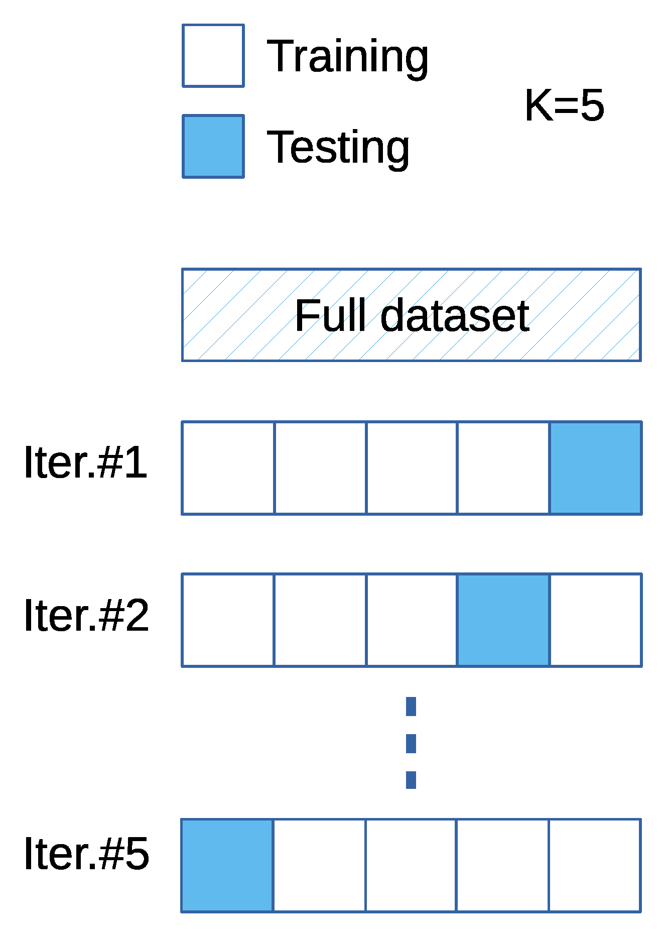
The traditional hold-out cross-validation (CV) technique, where the dataset is split into fixed training and testing datasets, is not practical for small datasets, as the testing dataset may contain important data features that are missed during the model training process. K-fold CV is advantageous, as it divides the whole database into K folds [34]. Then, the model is trained and tested K times separately; for every iteration, unique (K-1) folds are used as training data, and the remaining fold is used as the unseen testing dataset, as shown in Figure 3. The final model performance is calculated either from the best model or by averaging all the results.
However, for a biased dataset where the outputs are unevenly distributed throughout the range, stratified K-fold CV has been proven better [22]. Stratified K-fold CV ensures that data points in each fold cover the whole output range evenly. In this work, we performed stratified K-fold CV for K = 5 folds. We split the entire dataset into 15 subgroups based on the output distributions, then ensured that each fold contained data points from those 15 subgroups evenly.

3.1.5. Data Interpolation

Ideally, an effective machine learning (ML) model is trained with adequate and continuous data points [23]. Recently in the literature, several ML model implementations have been reported, where the original datasets were very small (<100 data points) due to the complication and high cost of the experiments in the biomedical engineering, chemical engineering, and material science domains [35,36,37]. Those models were trained with the assistance of interpolated data points to successfully overcome the issue of small and discontinuous datasets. In this work, we used the cubic-spline interpolation (CSI) technique to interpolate our small dataset (26 data points). In CSI, the data points are fitted with a piecewise function composed of several third-degree polynomial functions, where all polynomials and their first and second derivatives are continuous all over the dataset [38]. CSI performs better than other spatial interpolation techniques by providing a smother curve with fewer interpolation errors and no distortion in the boundary region [36,39]. The effectiveness of which technique has been proven in building various ML models for small datasets [36,37,40]. To interpolate data, we followed the CSI steps as described in [36].

3.1.6. ReLU

Rectified linear unit (ReLU) is a recently developed activation function for NNs that can be represented mathematically as [41]:
g x = max 0 , x = x   i f   x 0 0   i f   x < 0
ReLU has proven advantageous over traditional activation functions, such as sigmoid and hyperbolic tangent functions, as its first derivative ( g ( x ) ) is constant for  x 0 , overcoming the vanishing-gradient problem [29,41]. ReLU is used as the activation function for the hidden layers of our proposed NNs.

3.1.7. Model Evaluation

We used three metrics from the scikit-learn Python machine learning package to evaluate the performance of our deep learning neural network (DL-NN) models [42]: mean absolute error (MAE), root mean square error (RMSE), and coefficient of determination (R2). The fourth evaluation metric was the residual error (%). Among them, the residual error (%) is the simplest metric that shows the difference between the actual and predicted outcome out of 100:
R e s i d u a l   E r r o r   % = y i t r u e y i p r e d y i t r u e × 100
where  y i t r u e  is the i-th actual outcome, and  y i p r e d  is the i-th outcome predicted by the model.
MAE represents the mean of total absolute error:
M A E = 1 N i N y i t r u e y i p r e d
where N is the total number of data points.
RMSE is another standard metric used to evaluate the prediction performance of the model. It corresponds to the Euclidean distance between the predicted and true values:
R M S E = 1 N i N y i t r u e y i p r e d 2
R2 is a popular regression score function that provides a numerical value between 1 and 0, where 1 means that the model predicts the outcome perfectly, and 0 means that the model does not predict the outcome. R2 is calculated as:
R 2 = 1 i y i t r u e y i p r e d 2 i y i t r u e y ¯ t r u e 2
where  y ¯ t r u e  is the mean of the actual outcome.

3.1.8. Computational Framework

Training DLNN models consist of multiple layers of fully connected neurons and require a hardware platform that can perform extensive computations in parallel during every iteration. Rather using a local machine, in this work, the DLNN models are developed, trained, and tested using cloud based hardware resources provided by Google Collaboratory (Colab) [43]. Colab works based on Jupyter notebook service, which needs zero-setup and provides on-demand remote access to extensive computing resources, such as GPUs. Python 3.11.2 programming language and Keras API on the TensorFlow 2 platform were used to develop all the models in this work [44]. A Python library named Regressio under the MIT open-source license was used for the CSI of our dataset [45].

3.2. Model Development

In the current study, we built a DL-NN model to predict the stress, strain, elastic modulus, and toughness of PLA film. All these models have four inputs, which: weight percentage (wt%) of PLA, wt% of HKUST-1, casting thickness (µm), and immersion time (minutes). The flow chart presented in Figure 4 demonstrates the steps of the workflow for the proposed work:

3.2.1. Data Preprocessing

We started data preprocessing by normalizing our dataset’s input and output parameters, a common practice before DL-NN training [46]. Next, we interpolated data points following the CSI technique to ensure that we had enough data points spread over the entire input space in which the model was to be applied [36,46]. Our original dataset comprised 26 data points and four output parameters. We interpolated 1214 data points in total: 286, 288, 338, and 302 data points for the DL-NN models to predict the stress, strain, elastic modulus, and toughness, respectively. The interpolated data were used for model tuning, training, and cross-validation purposes, whereas the original 26 data points were kept isolated only for testing purposes. Stratified K-fold CV allowed us to use all 1214 interpolated data points for training and validation/testing purposes.

3.2.2. Tuning Hyperparameters and Model Selection

We used the grid search method to individually tune the critical hyperparameters of the Keras-based DL-NNs, such as the number of hidden layers, number of neurons, kernel initializer, activation function, model optimizer, learning rate, number of epochs, and dropout rate. First, a set of proper ranges/options were selected as grids for each of these parameters. Then, each of the grids was evaluated 4–5 times to determine the actual model performance. Finally, the best grid options for all the hypermeters were selected for the training phases. In Appendix A, we summarize all the tuned hyperparameters for our DL-NNs. The selected DL-NN model has 4 hidden layers, with a total of 40 neurons distributed in a 4-(16-12-8-4)-4 architecture, as shown in Figure 5, where ReLU is the activation function for the hidden layers, and a linear activation function is used for the output layer [41].
We used the NN illustrated above with the hyperparameters mentioned in Table A1 to build four individual regression models for each output of our dataset.

3.2.3. Training the Models

The four models used to predict each output were trained separately with their corresponding interpolated data, obtaining their optimized weight metrics. Identical training procedures were followed for each model, initiated by splitting the interpolated data into five sets following stratified K-fold CV for K = 5 folds. Then, the model was trained in 5 iterations, and the evaluation performance was noted in terms of MAE, MSE, and R2. MAE was the loss function used to train all models. Each iteration used the corresponding stratified 4 folds as the training dataset. The dropout and early stopping techniques were applied to prevent overfitting and generalize the model performance [29,30,33,35]. After completing the 5 iterations, the best-trained mode in terms of the evaluation metrics was chosen for the testing phases.

3.2.4. Testing and Performance Analysis of the Trained Models

The 4 selected and trained models of each output were tested with the original dataset, which was unknown during the model training phases. The trained models were also tested with the unseen interpolated data fold, i.e., the unused 1 fold of data points during the training iteration of the selected model. Finally, data were analyzed and presented.

4. Results and Discussion

4.1. Dataset Analysis

As previously mentioned, we applied CSI techniques to interpolate the original dataset. Table 3 shows the statistical properties of all the output parameters in the original and interpolated datasets, and Figure 6 shows their distribution in detail. The original dataset not only has a small number of data points, but their distribution is also uneven and discontinuous. However, in order to build an effective NN model, the dataset needs to be continuous all over the range and sufficiently large [23,35]. We can also see from Figure 6 that the interpolated dataset meets these requirements. Table 3 shows that the min. and max. of all the output parameters are identical in most cases between the original and interpolated dataset. Conversely, we see differences in their means and standard deviations with redistribution of the data points evenly without discontinuity for the interpolated dataset.

4.2. Model Generalization

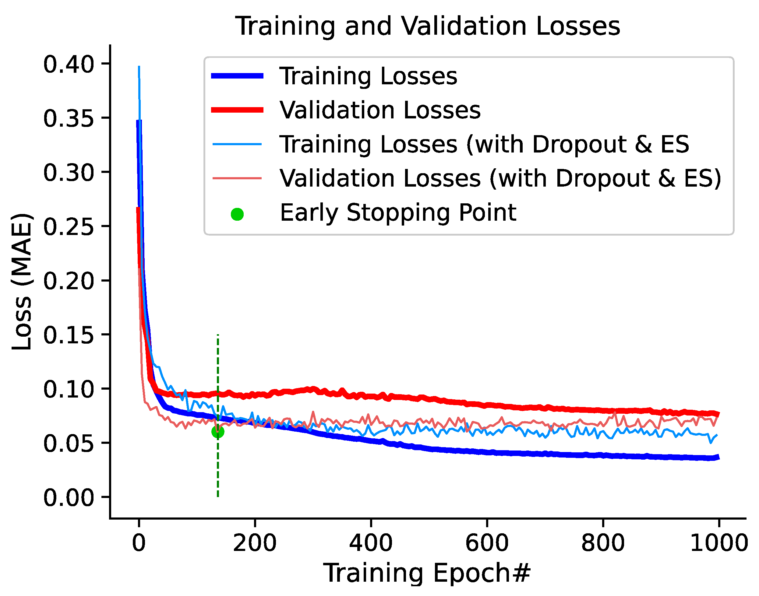
In the proposed work, all the models were generalized and optimized from the over fittings by applying the dropout and ES regularization techniques. For example, Figure 7 shows the training and validation losses for the E model of iteration #3 with and without the dropout and ES regularizations. When there was no regularization, the training loss reached <0.05 MAE after convergence, which is the minimum reported MAE in this figure. However, at that point, the validation loss was ~0.10 MAE, which is 100% more than the training loss. Optimum validation loss is crucial, as it indicates the model’s efficiency for the unknown dataset [24,30]. This significant difference between the training and validation loss suggests the model was overfitted and follows the training data instead of extracting the data features. Figure 7 also shows that this overfitting issue is overcome when we train the same model with the dropout and ES regulations. This approach generalized the model’s evaluation performance for the known (training) and unknown (validation) data. It also reduced the validation loss up to ~0.06 MAE, which is 40% less than the validation loss reported for the model without dropouts and ES. It is also observed from this figure that the validation loss reached its minimum before the training loss fully converged, as indicated by the green dot. Subsequently, as we trained the model for more epochs, the training loss decreased gradually, while the validation loss slightly increased, ES provided the advantage of stopping the training process when the validation loss was optimum.

4.3. Performance Evaluation

Table 4 compares the evaluation performances of the four DL-NN models for the prediction of stress, strain, E, and toughness in terms of MAE, MSE, and R2. We evaluated each model using three types of datasets: (type 1) the known interpolated data point folds used in the model, (type 2) the unknown interpolated data point folds used in the model, and (type 3) the original data points, which were also unknown to the model. All the models performed identically for the type-1 and type-2 datasets: MSE, 0.39–0.59; RMSE, 0.045–0.071; R2, 0.93–0.97. We believe these similar model performances for the known and unknown interpolated datasets were archived due to the dropout and ES techniques, as shown in Figure 7. The same statistical properties of the interpolated data points in for type 1 and type 2 is another reason for the similar performances. The three rightmost columns in Table 4 summarize the model performance for the type-3 dataset. The evaluation performance of all models dropped compared to that of type-1 and type-2 datasets, but they still maintained a satisfactory level [47]: MSE, 0.48–0.062; RMSE, 0.063–0.095; R2, 0.78–0.88. We can attribute this performance dropoff to the statistical differences between the interpolated and original datasets, as visible in Table 3 and Figure 6. The main objective of data interpolation in this work was to generate sufficient and continuous data points with the same features as the original dataset, not necessarily with the same statistical properties. Table 4 also shows that the evaluation performance of the toughness model is slightly less accurate than that the three other output models for type-1, type-2, and type-3 datasets. The typically reduced performance of the toughness model can be linked to one of the following assumptions: the toughness of the PLA film has a relatively weaker correlation with all input parameters of our dataset or measurement errors exists within the toughness data [48].
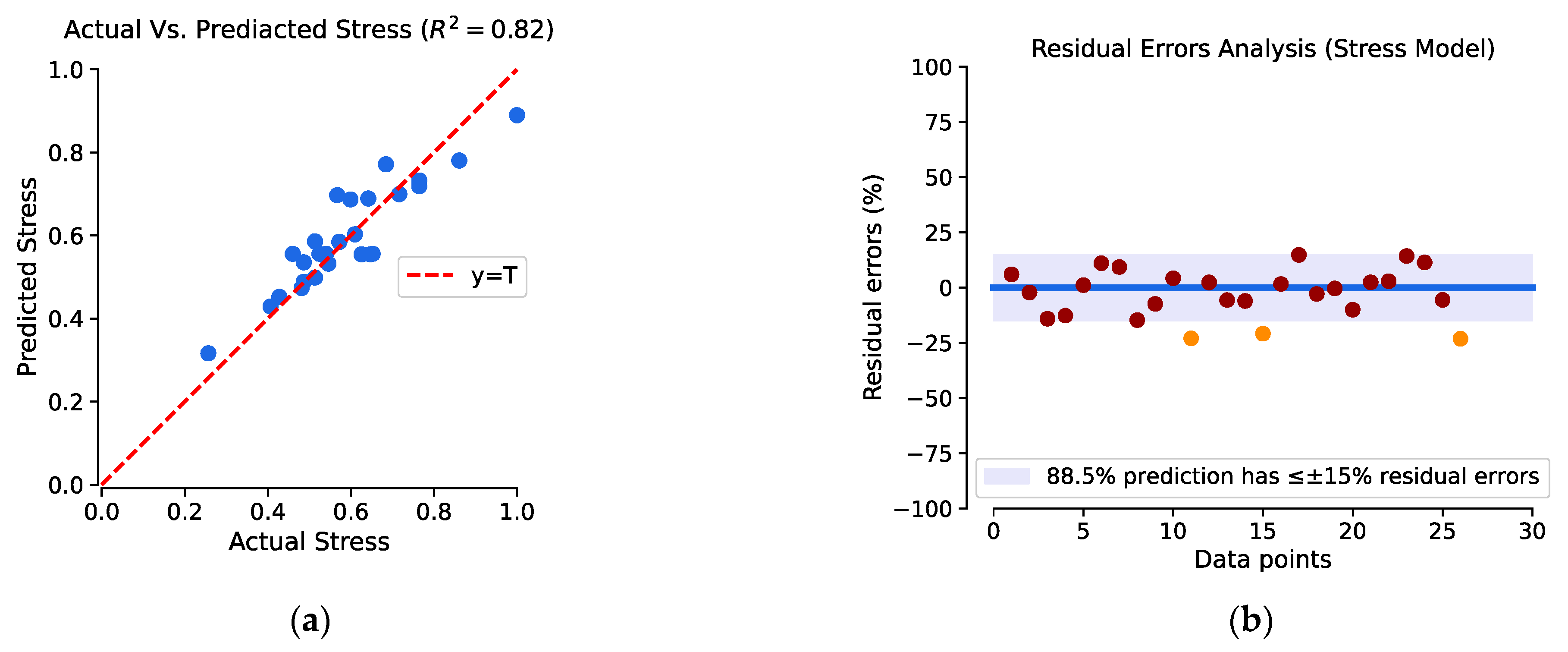
Figure 8 shows a graphic representation of the prediction performances and residual errors of the stress, strain, E, and toughness models for the original data points and those unknown to the model (i.e., type-3 dataset). Figure 8a,c,e,g show that the perfect prediction line (y = T) closely surrounds the predictions of all the models, and Figure 8b,d,f,h show that the majority of the predictions have <±15% residual errors. The strain model has the best R2 score of 0.88: 73.1% of its predictions have <±15% residual errors—the third-best residual error performance compared to the other models. Figure 6b,c show that this mode predicted the larger strains in the 0.4–1 range more precisely, whereas for the smaller strains, the prediction contained more errors. The stress model showed the best performance in terms of residual errors, i.e., 88.5% of its predictions had < ±15% residual errors, but its R2 score was 0.82, which is the second-best among all the modes. Figure 6a,b indicate the reason for this; the model achieves consistent prediction performance all over the stress range of 0–1, with a certain percentage of moderate error. The toughness model exhibited the worse performance regarding the R2 score and residual errors, as evident in Table 2.
To summarize the discussion, we generated sufficiently large and continuous interpolated data points by mimicking the data features of the original dataset by applying CSI techniques. Then, the interpolated data were used in the training phases so that our NN models could extract and learn the data features and predict the outputs from the unknown original dataset. Table 2 and Figure 8 show that our models achieved satisfactory precision in predicting the unknown data points, regardless of whether they belonged to the interpolated or original dataset.

5. Conclusions

We developed a DLNN model to predict four mechanical properties of the PLA/HKUST-1 MMM: stress, strain, elastic modulus, and toughness. The model was developed using the TensorFlow 2 backend Keras API in Python programming language. A total of 1214 CSI data points were generated from the 26 experimental data points reported in [13] and split into stratified K-fold CV of five folds to train and validate the mode. The grid search methods were used to tune all the model hyperparameters. Dropout and early stopping regulation were used to generalize the model and optimize the overfitting issues during model training. Finally, the model was tested using unknown CSI data point folds and experimental data points. The model’s R2 score was between 0.9 and 0.97 for the CSI data points and between 0.78 and 0.88 for the experimental data points. In both cases, the model achieved the highest score for strain prediction and the lowest score for toughness prediction. The distinctiveness of this work is that we demonstrated the performance of our model for the full range of experimental data points, unlike in other recent works, as illustrated in Table 1. This also suggests that following our proposed method, an effective NN model can be built using a small dataset for prediction of material properties.

Author Contributions

Conceptualization, Z.A.A., M.A.M. and S.R.; methodology, M.A.M. and S.R.; software, M.A.M.; validation, M.A.M. and S.R.; formal analysis, M.A.M. and S.R.; investigation, Z.A.A., M.A.M. and S.R.; resources, Z.A.A. and M.A.M.; data curation, Z.A.A. and M.A.M.; writing—original draft preparation, M.A.M. and S.R.; writing—review and editing, Z.A.A., M.A.M. and S.R.; visualization, M.A.M.; supervision, S.R.; project administration, Z.A.A. and S.R.; funding acquisition, Z.A.A. and S.R. All authors have read and agreed to the published version of the manuscript.

Funding

This research, including the APC, was funded by the Deanship of Scientific Research, King Faisal University, grant number 4005.

Data Availability Statement

The data are available in [13].

Acknowledgments

This work was supported through the Ambitious Research Track by the Deanship of Scientific Research, Vice Presidency for Graduate Studies and Scientific Research, King Faisal University, Saudi Arabia [Project No. GRANT4005]. The authors would like to acknowledge the technical and instrumental support they received from King Faisal University, Qassim University, and University of Nottingham.

Conflicts of Interest

The authors declare no conflict of interest.

Appendix A. Tuned Hyperparameters

Table A1 summarizes all the tuned hyperparameters used to train and test out DL-NN models.
Table A1. Tuned hyperparameters the DL-NNs.
HyperparameterTuning Option
Hidden layers4
Neurons40
Kernel initializerGlorotNormal
Activation functionReLU (for hidden layers)
Linear (for output layers)
Model optimizerAdam
Learning rate10−4 (for NN model without dropout)
10−3 (for NN model with dropout)
Loss functionMSE
Epochs1000–1500
Dropout rateStress modeling: 7–8%
Strain modeling: 4–5%
E modeling: 12–15%
Toughness modeling: 10–13%

References

  1. La Rosa, D. Life cycle assessment of biopolymers. In Biopolymers and Biotech Admixtures for Eco-Efficient Construction Materials; Pacheco-Torgal, F., Ivanov, V., Karak, N., Jonkers, H., Eds.; Woodhead Publishing: Sawston, UK, 2016; pp. 57–78. [Google Scholar] [CrossRef]
  2. Sternberg, J.; Sequerth, O.; Pilla, S. Green chemistry design in polymers derived from lignin: Review and perspective. Prog. Polym. Sci. 2021, 113, 101344. [Google Scholar] [CrossRef]
  3. Muneer, F.; Nadeem, H.; Arif, A.; Zaheer, W. Bioplastics from Biopolymers: An Eco-Friendly and Sustainable Solution of Plastic Pollution. Polym. Sci. Ser. C 2021, 63, 47–63. [Google Scholar] [CrossRef]
  4. Kumari, S.V.G.; Pakshirajan, K.; Pugazhenthi, G. Recent advances and future prospects of cellulose, starch, chitosan, polylactic acid and polyhydroxyalkanoates for sustainable food packaging applications. Int. J. Biol. Macromol. 2022, 221, 163–182. [Google Scholar] [CrossRef] [PubMed]
  5. Ilyas, R.A.; Sapuan, S.M.; Harussani, M.M.; Hakimi, M.Y.A.Y.; Haziq, M.Z.M.; Atikah, M.S.N.; Asyraf, M.R.M.; Ishak, M.R.; Razman, M.R.; Nurazzi, N.M.; et al. Polylactic Acid (PLA) Biocomposite: Processing, Additive Manufacturing and Advanced Applications. Polymers 2021, 13, 1326. [Google Scholar] [CrossRef] [PubMed]
  6. Bioplastics Market Development Update 2019. Available online: https://www.european-bioplastics.org/wp-content/uploads/2019/11/Report_Bioplastics-Market-Data_2019_short_version.pdf (accessed on 10 June 2023).
  7. Chung, T.-S.; Jiang, L.Y.; Li, Y.; Kulprathipanja, S. Mixed matrix membranes (MMMs) comprising organic polymers with dispersed inorganic fillers for gas separation. Prog. Polym. Sci. 2007, 32, 483–507. [Google Scholar] [CrossRef]
  8. Shah, M.; McCarthy, M.C.; Sachdeva, S.; Lee, A.K.; Jeong, H.-K. Current Status of Metal–Organic Framework Membranes for Gas Separations: Promises and Challenges. Ind. Eng. Chem. Res. 2012, 51, 2179–2199. [Google Scholar] [CrossRef]
  9. Li, Y.; Fu, Z.; Xu, G. Metal-organic framework nanosheets: Preparation and applications. Coord. Chem. Rev. 2019, 388, 79–106. [Google Scholar] [CrossRef]
  10. Knebel, A.A.; Caro, J. Metal–organic frameworks and covalent organic frameworks as disruptive membrane materials for energy-efficient gas separation. Nat. Nanotechnol. 2022, 17, 911–923. [Google Scholar] [CrossRef]
  11. Richardson, N. Investigating Mechano-Chemical Encapsulation of Anti-cancer Drugs on Aluminum Metal-Organic Framework Basolite A100—ProQuest. Master’s Thesis, Morgan State University, Baltimore, MD, USA, 2021. Available online: https://www.proquest.com/openview/9adc81f41808abbc2bf9a503d2095a45 (accessed on 10 June 2023).
  12. Lin, R. MOFs-Based Mixed Matrix Membranes for Gas Separation. Ph.D. Thesis, The University of Queensland, Saint Lucia, Australia, 2016. Available online: https://core.ac.uk/reader/83964620 (accessed on 10 June 2023).
  13. Alhulaybi, Z.A. Fabrication of Porous Biopolymer/Metal-Organic Framework Composite Membranes for Filtration Applications. Ph.D. Thesis, University of Nottingham, Nottingham, UK, 2020. Available online: https://eprints.nottingham.ac.uk/63048/ (accessed on 10 June 2023).
  14. Stănescu, M.M.; Bolcu, A. A Study of the Mechanical Properties in Composite Materials with a Dammar Based Hybrid Matrix and Reinforcement from Crushed Shells of Sunflower Seeds. Polymers 2022, 14, 392. [Google Scholar] [CrossRef]
  15. Soltane, H.B.; Roizard, D.; Favre, E. Effect of pressure on the swelling and fluxes of dense PDMS membranes in nanofiltration: An experimental study. J. Membr. Sci. 2013, 435, 110–119. [Google Scholar] [CrossRef]
  16. Miao, Z.; Ji, X.; Wu, M.; Gao, X. Deep learning-based evaluation for mechanical property degradation of seismically damaged RC columns. Earthq. Eng. Struct. Dyn. 2023, 52, 2498–2519. [Google Scholar] [CrossRef]
  17. Gyurova, L.A. Sliding Friction and Wear of Polyphenylene Sulfide Matrix Composites: Experimental and Artificial Neural Network Approach. Ph.D. Thesis, Technische Universität Kaiserslautern, Kaiserslautern, Germany, 2010. Available online: https://kluedo.ub.rptu.de/frontdoor/index/index/docId/4717 (accessed on 10 June 2023).
  18. Sterjovski, Z.; Nolan, D.; Carpenter, K.R.; Dunne, D.P.; Norrish, J. Artificial neural networks for modelling the mechanical properties of steels in various applications. J. Mater. Process. Technol. 2005, 170, 536–544. [Google Scholar] [CrossRef]
  19. Park, S.; Marimuthu, K.P.; Han, G.; Lee, H. Deep learning based nanoindentation method for evaluating mechanical properties of polymers. Int. J. Mech. Sci. 2023, 246, 108162. [Google Scholar] [CrossRef]
  20. Merayo, D.; Rodríguez-Prieto, A.; Camacho, A.M. Prediction of Mechanical Properties by Artificial Neural Networks to Characterize the Plastic Behavior of Aluminum Alloys. Materials 2020, 13, 5227. [Google Scholar] [CrossRef]
  21. Kazi, M.-K.; Eljack, F.; Mahdi, E. Optimal filler content for cotton fiber/PP composite based on mechanical properties using artificial neural network. Compos. Struct. 2020, 251, 112654. [Google Scholar] [CrossRef]
  22. Charilaou, P.; Battat, R. Machine learning models and over-fitting considerations. World J. Gastroenterol. 2022, 28, 605–607. [Google Scholar] [CrossRef] [PubMed]
  23. Zhang, Y.; Ling, C. A strategy to apply machine learning to small datasets in materials science. npj Comput. Mater. 2018, 4, 25. [Google Scholar] [CrossRef]
  24. Marin, A.; Skelin, K.; Grujic, T. Empirical Evaluation of the Effect of Optimization and Regularization Techniques on the Generalization Performance of Deep Convolutional Neural Network. Appl. Sci. 2020, 10, 7817. [Google Scholar] [CrossRef]
  25. Feng, S.; Zhou, H.; Dong, H. Using deep neural network with small dataset to predict material defects. Mater. Des. 2019, 162, 300–310. [Google Scholar] [CrossRef]
  26. Song, H.; Ahmad, A.; Farooq, F.; Ostrowski, K.A.; Maślak, M.; Czarnecki, S.; Aslam, F. Predicting the compressive strength of concrete with fly ash admixture using machine learning algorithms. Constr. Build. Mater. 2021, 308, 125021. [Google Scholar] [CrossRef]
  27. Long, X.; Mao, M.; Lu, C.; Li, R.; Jia, F. Modeling of heterogeneous materials at high strain rates with machine learning algorithms trained by finite element simulations. J. Micromech. Mol. Phys. 2021, 6, 2150001. [Google Scholar] [CrossRef]
  28. Jha, K.; Jha, R.; Jha, A.K.; Hassan, M.A.M.; Yadav, S.K.; Mahesh, T. A Brief Comparison On Machine Learning Algorithms Based On Various Applications: A Comprehensive Survey. In Proceedings of the 2021 IEEE International Conference on Computation System and Information Technology for Sustainable Solutions (CSITSS), Bangalore, India, 16–18 December 2021; pp. 1–5. [Google Scholar] [CrossRef]
  29. Liu, G.; Bao, H.; Han, B. A Stacked Autoencoder-Based Deep Neural Network for Achieving Gearbox Fault Diagnosis. Math. Probl. Eng. 2018, 2018, e5105709. [Google Scholar] [CrossRef]
  30. Srivastava, N.; Hinton, G.; Krizhevsky, A.; Sutskever, I.; Salakhutdinov, R. Dropout: A simple way to prevent neural networks from overfitting. J. Mach. Learn. Res. 2014, 15, 1929–1958. [Google Scholar]
  31. Wang, S.; Manning, C. Fast dropout training. In Proceedings of the 30th International Conference on Machine Learning, Atlanta, GA, USA, 16–21 June 2013; pp. 118–126. Available online: https://proceedings.mlr.press/v28/wang13a.html (accessed on 10 June 2023).
  32. Prechelt, L. Early Stopping—But When? In Neural Networks: Tricks of the Trade; Orr, G.B., Müller, K.-R., Eds.; Lecture Notes in Computer Science; Springer: Berlin/Heidelberg, Germany, 1998; pp. 55–69. [Google Scholar] [CrossRef]
  33. Ji, Z.; Li, J.; Telgarsky, M. Early-stopped neural networks are consistent. In Proceedings of the 35th Conference on Neural Information Processing Systems, Virtual, 6–14 December 2021. [Google Scholar]
  34. Bhagat, M.; Bakariya, B. Implementation of Logistic Regression on Diabetic Dataset using Train-Test-Split, K-Fold and Stratified K-Fold Approach. Natl. Acad. Sci. Lett. 2022, 45, 401–404. [Google Scholar] [CrossRef]
  35. Shaikhina, T.; Lowe, D.; Daga, S.; Briggs, D.; Higgins, R.; Khovanova, N. Machine Learning for Predictive Modelling based on Small Data in Biomedical Engineering. IFAC-PapersOnLine 2015, 48, 469–474. [Google Scholar] [CrossRef]
  36. Hafsa, N.; Rushd, S.; Al-Yaari, M.; Rahman, M. A Generalized Method for Modeling the Adsorption of Heavy Metals with Machine Learning Algorithms. Water 2020, 12, 3490. [Google Scholar] [CrossRef]
  37. Podder, S.; Majumder, C.B. The use of artificial neural network for modelling of phycoremediation of toxic elements As(III) and As(V) from wastewater using Botryococcus braunii. Spectrochim. Acta Part A Mol. Biomol. Spectrosc. 2016, 155, 130–145. [Google Scholar] [CrossRef]
  38. Biran, A. (Ed.) Chapter 7—Cubic Splines. In Geometry for Naval Architects; Butterworth-Heinemann: Oxford, UK, 2019; pp. 305–324. [Google Scholar] [CrossRef]
  39. Artley, B. Cubic Splines: The Ultimate Regression Model. Medium. 4 August 2022. Available online: https://towardsdatascience.com/cubic-splines-the-ultimate-regression-model-bd51a9cf396d (accessed on 20 April 2023).
  40. Won, W.; Lee, K.S. Adaptive predictive collocation with a cubic spline interpolation function for convection-dominant fixed-bed processes: Application to a fixed-bed adsorption process. Chem. Eng. J. 2011, 166, 240–248. [Google Scholar] [CrossRef]
  41. Ding, B.; Qian, H.; Zhou, J. Activation functions and their characteristics in deep neural networks. In Proceedings of the 2018 Chinese Control and Decision Conference (CCDC), Shenyang, China, 9–11 June 2018; pp. 1836–1841. [Google Scholar] [CrossRef]
  42. Scikit-Learn: Machine Learning in Python—Scikit-Learn 1.2.2 Documentation. Available online: https://scikit-learn.org/stable/index.html (accessed on 20 April 2023).
  43. Google Colaboratory. Available online: https://colab.research.google.com/ (accessed on 22 April 2023).
  44. Keras: Deep Learning for Humans. Available online: https://keras.io/ (accessed on 22 April 2023).
  45. Artley, B. Regressio. Available online: https://github.com/brendanartley/Regressio (accessed on 11 June 2023).
  46. Hagan, M.T.; Demuth, H.B.; Beale, M.H.; Jesús, O.D. Neural Network Design, 2nd ed.; Martin Hagan: San Francisco, CA, USA, 2014. [Google Scholar]
  47. Moore, D.S.; Notz, W.I.; Fligner, M.A. The Basic Practice of Statistics, 6th ed.; W. H. Freeman: New York, NY, USA, 2011. [Google Scholar]
  48. Cheng, C.-L.; Shalabh; Garg, G. Coefficient of determination for multiple measurement error models. J. Multivar. Anal. 2014, 126, 137–152. [Google Scholar] [CrossRef]
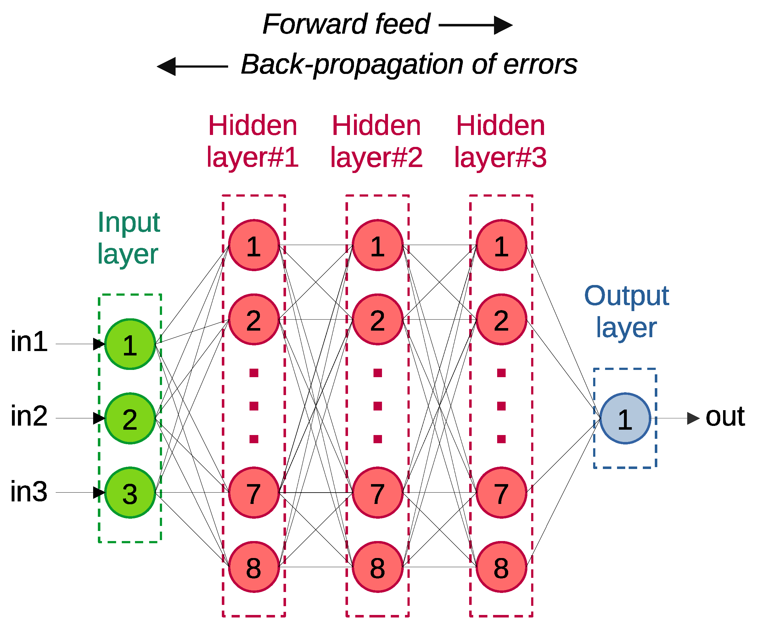
Figure 1. A DNN model with a 3-(8-8-8)-1 architecture.
Chemengineering 07 00080 g001
Figure 2. (a) A simple NN model with two hidden layers. (b) Dropout randomly deactivates neurons while training the NN model.
Chemengineering 07 00080 g002
Figure 3. K-fold CV/stratified K-fold CV for K = 5.
Chemengineering 07 00080 g003
Figure 4. Flow chart demonstrating the workflow of the proposed work.
Chemengineering 07 00080 g004
Figure 5. Selected DL model with 4-(16-12-8-4)-4 NN architecture.
Chemengineering 07 00080 g005
Figure 6. Data point distribution of original dataset and interpolated dataset for (a) stress, (b) strain, (c) elastic modulus (E), and (d) toughness.
Chemengineering 07 00080 g006
Figure 7. Dropout and ES techniques used to generalize the models for the training data (known) and validation data (unknown).
Chemengineering 07 00080 g007
Figure 8. Visualizing the prediction performances and residual errors (%) for the stress model (a,b), the strain model (c,d), the E model (e,f), and the toughness model (g,h) using a type-3 dataset (i.e., the original data points and those unknown to the model). In (b,d,f,h), the brown dots are the predictions with  ± 15 %  residual errors, yellow dots are the predictions with  > ± 15 %  residual errors, and the blue line represents the 0% residual errors.
Chemengineering 07 00080 g008aChemengineering 07 00080 g008b
Table 2. Results of experimental measurements.
Input 1Input 2Input 3Input 4Output 1Output 2Output 3Output 4
PLA wt%HKUST-1 wt%Casting Thickness (µm)Immersion Time (min)Stress (MPa)StrainE (MPa)Toughness (KJ/m3)
100015014401.430.1139.3010.26
1000150901.070.13279.94
1000150100.960.0830.404.48
100010014401.280.1632.3015.61
1000100901.140.1623.9011.96
1000100101.870.1842.5021.90
10005014401.610.0860.8012.07
100050901.120.0652.507.53
100050101.20.0846.707.68
10002514401.430.0765.207.32
100025901.060.0448.503.25
100025101.340.0843.506.85
95515014400.800.1026.606.98
955150900.980.0930.104.80
955150100.860.0830.704.37
95510014400.900.1225.708.65
955100901.220.08379.72
955100101.010.0627.603.65
9555014400.910.1318.609.80
95550900.910.0539.503.64
95550101.020.0441.603.68
9552514400.960.0445.702.57
95525901.210.04494.78
95525101.170.0544.704.72
901050900.760.0539.543.64
802050900.480.0518.681.78
Table 3. Statistical properties of the original and interpolated data points for stress, strain, elastic modulus, and toughness.
Statistical PropertiesOriginal DatasetInterpolated Dataset
Stress
(MPa)
StrainElastic Modulus
(MPa)
Toughness
(Kj/m3)
Stress
(MPa)
StrainElastic Modulus
(MPa)
Toughness
(Kj/m3)
Data Points26262626286288338302
Min.0.480.0418.601.780.460.0416.601.28
Max.1.870.1865.221.91.890.1867.1522.35
Mean1.100.0937.997.371.170.1141.8811.82
Std. Deviation0.290.0412.034.540.410.0414.666.11
Table 4. Evolution of the models using known interpolated, unknown interpolated, and unknown original datasets.
#Modeling OutputDropout RateModel Performance Evaluation
Using Type-1 Dataset (Known
Interpolated Data Points)
Using Type-2 Dataset (Unknown Interpolated Data Points)Using Type-3 Dataset (Unknown Original Data Points)
MAERMSER2MAERMSER2MAERMSER2
1Stress7.5%0.040.050.950.040.050.950.050.060.82
2Strain4.5%0.030.050.970.030.050.970.050.080.88
3Elastic modulus12.5%0.040.050.960.040.050.960.050.070.82
4Toughness11.5%0.060.070.930.060.070.930.060.100.78
Disclaimer/Publisher’s Note: The statements, opinions and data contained in all publications are solely those of the individual author(s) and contributor(s) and not of MDPI and/or the editor(s). MDPI and/or the editor(s) disclaim responsibility for any injury to people or property resulting from any ideas, methods, instructions or products referred to in the content.