Streamflow Trends in Central Chile

Abstract

The availability of water in Chile has shown signs of decline in recent decades. This is problematic because Chile’s economy depends on mining, forestry, and agricultural activities, all limited by the availability of water resources. In this study, daily, monthly and annual flows in 31 basins located in the arid–semiarid zones (29°12′ S–33°58′ S) and in the humid–subhumid zones (34°43′ S–38°30′ S) of Chile were evaluated using the Mann–Kendall trend test and the quantile–Kendall procedure during three periods: 1984–2021 (31 stations), 1975–2021 (20 stations), and 1969–2021 (18 stations). Results showed that, at the annual level, trends were predominantly negative in both climatic zones and over the three periods analyzed. In the arid–semiarid zone, a higher frequency of annual significant negative trends was found in maximum flows in 1969–2021 and 1975–2021, compared to the last period under study. The humid–subhumid zone showed significant annual negative trends in all series analyzed. At the monthly level, on the other hand, the arid-semiarid zone showed a decrease in significant negative trends as the number of years analyzed increased, for all flow types. The humid–subhumid zone did not indicate a similar defined pattern. Likewise, the quantile–Kendall procedure showed a reduction in the significant trends as the length of the time series was increased in the arid-semiarid zone, but no such pattern was observed in the humid–subhumid zone. Furthermore, a relationship was observed for the PDO and the summer month flows for both zones. Consequently, it is concluded that the flow trends are generally negative, and their statistical significance depends on the period studied.

1. Introduction

Scientific evidence suggests that the world’s atmosphere has experienced an increase in temperatures [1,2,3] and because Chile is in a climate transition zone [4], the phenomenon of climate change could have a very high impact in this South American country, particularly for the availability and use of surface water resources. Thus, the influence of this phenomenon on peak-flow behaviors could increase, as this important hydrologic variable is extremely sensitive to climatic behaviors [5,6].

Hydrological variables such as rainfall and runoff are impacted by climate change, raising concerns about their behavior in future scenarios, because they are directly influenced by broad temporal and spatial phenomena [7,8]. In this sense, Carrasco et al. [9,10], for example, analyzed the tendencies of the 0 °C isotherm in central Chile, a climatic variable that directly affects the snow–glacial hydrologic behavior, concluding that it has increased its elevation over time, i.e., there has been an increase in temperature [9,11,12] and, consequently, the volume that was previously precipitated as snow is now most likely transformed directly into surface runoff.

Floods are natural processes, with no periodicity and caused by a significant and sudden increase in flowrates in a fluvial system, which involves a rise of water levels that can overflow river banks and then progressively occupy the land above it, flowing into the surrounding land [13,14,15,16,17]. According to Paoli et al. [18], floods that occur in hydrological terms have a different degree of risk and a different probability of exceedance, depending on peak-flow rates, volumes, or durations considered.

Countless studies around the world focusing on hydrological tendencies have been carried out in recent decades, many of which confirming clear behavioral changes (e.g., [19,20,21,22]). In Chile, however, this important topic is not well understood. Among the most relevant conclusions are those by Novoa et al. [19,20], who analyzed streamflow tendencies in the Coquimbo region (northern Chile), finding mostly positive tendencies, most likely due to glacier melting processes. Similarly, Pellicciotti et al. [21] analyzed mean monthly streamflow rates for the Aconcagua river (Valparaíso region, Central Chile), finding negative tendencies in surface water production, a conclusion supported by Givovich [23] and Martínez et al. [22], who verified similar behaviors for mean annual and monthly streamflow rates, respectively. Souvignet et al. [24], on the other hand, studied annual and seasonal temperature, precipitation, and flow tendencies in the Coquimbo region, concluding that only two out of the nine watersheds involved had a negative and significant annual tendency. Seasonally speaking, winter had more significant tendencies (in three watersheds). Nevertheless, the authors considered a time period ending in 2006, which motivates the need to revisit these studies using recent hydrological data, particularly in the context of a climate change scenario and given the current megadrought that is straining Chile’s freshwater resources to the breaking point.

Therefore, it is crucial to determine if streamflows (min, mean, and max) of watersheds in central Chile have had significant variation in recent decades, which may potentially be driven by climate change. In this context, this study intends to evaluate streamflow trends for different temporal periods and in different watersheds in central Chile.

2. Materials and Methods

2.1. Study Area

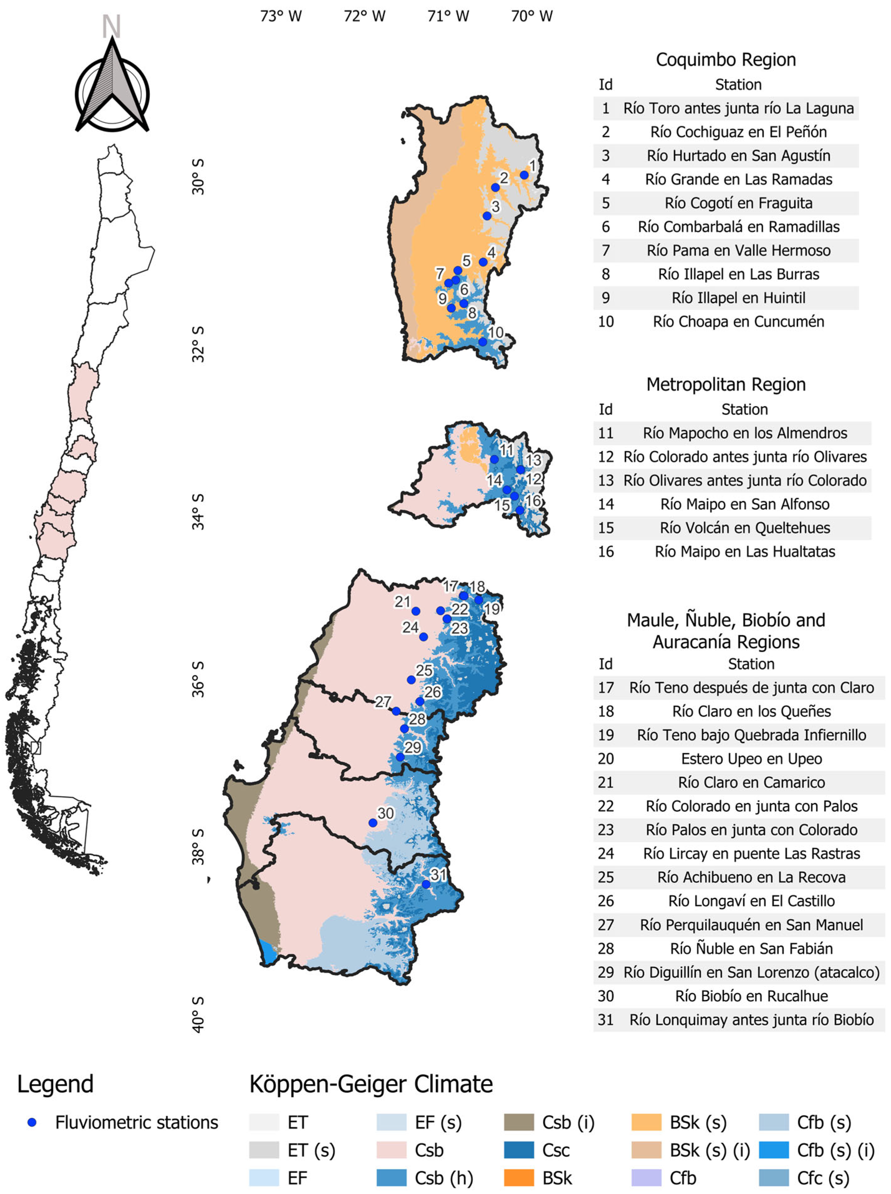
The study area comprised 31 watersheds (or fluviometric stations) distributed within central Chile, all distributed in the Coquimbo, Metropolitana, Maule, Ñuble, Biobío, and Araucanía administrative regions (Figure 1). In terms of climate, according to the Köppen–Geiger climate classification [25], the Coquimbo region presents a cold, arid climate between 29°00′ and 30°00′ south latitude, and a warm, arid climate between 30°00′ and 32°00′ south latitude. The remaining regions (Metropolitana, Maule, Ñuble, Biobío, and Araucanía) share a Mediterranean oceanic climate type, characterized by wet winters and long dry summers. However, the Metropolitana region has a semiarid climate type as well, whereas Maule and Biobío have humid and subhumid climates, respectively. As illustrated in Figure 1, a small portion of the study area is classified as tundra climate. Thus, each region differs from each other in terms of area and climate (

Table 1. Characteristics of each region.

Region	Area (km2)	Climate	Mean Annual Precipitation (mm)
Coquimbo	40,580	Arid	50–300
Metropolitana	15,403	Semiarid	200–700
Maule	30,296	Subhumid	500–2000
Ñuble	13,179	Humid	1000–2000
Biobío	24,022	Humid	1200–2000
Araucanía	31,842	Humid	1500–2500

).

2.2. Dataset

The information used for this study was obtained from the General Water Directorate (DGA) and includes daily mean streamflows and monthly minimum, mean, and maximum streamflow rates. Stations from watersheds without anthropic intervention (such as the upstream presence of reservoirs or irrigation channels) were selected from DGA’s hydrological database. Moreover, the stations represent very diverse drainage areas, ranging from 113 to 7044 km². Finally, no data completion was carried out where missing data were encountered in the series. Furthermore, the DGA periodically collects, manages, and verifies the quality of the instruments and data.

Table 2. Fluviometric stations (for each climate type) and periods with available records.

Zone	ID	1969–2021	1975–2021	1984–2021
Arid–semiarid	1			✓
	2			✓
	3	✓	✓	✓
	4	✓	✓	✓
	5	✓	✓	✓
	6		✓	✓
	7			✓
	8	✓	✓	✓
	9	✓	✓	✓
	10	✓	✓	✓
	11			✓
	12		✓	✓
	13			✓
	14	✓	✓	✓
	15	✓	✓	✓
	16			✓
Humid–subhumid	17	✓	✓	✓
	18			✓
	19			✓
	20			✓
	21	✓	✓	✓
	22	✓	✓	✓
	23	✓	✓	✓
	24	✓	✓	✓
	25			✓
	26	✓	✓	✓
	27	✓	✓	✓
	28	✓	✓	✓
	29	✓	✓	✓
	30	✓	✓	✓
	31			✓

shows the fluviometric stations and the years used in the study, based on the data provided by the DGA, for each station. Table 2 shows the number of fluviometric stations with historic data, which were divided between the years involved (1984–2021) and the years for which it was extended for a second analysis, with 40 years (1975–2021) and with 46 years (1969–2021), given the available data.

Table 2 shows the total number of stations analyzed for periods between 1984 and 2021, and with a further 9 and 15 years of extension, respectively. By extending the data series 9 more years, the analysis period 1975–2021 was defined; however, the number of stations that could be analyzed was reduced to 20. Similarly, by extending the data series 15 more years, the period 1969–2021 was defined and the number of stations available for analysis was reduced to 18.

Hence, the data series used in this study represented mostly data from recent fluviometric stations, many of which began collecting data in the 1980s, even though there were even newer stations available. All of these stations were considered valid only for the analysis of the 1984–2021 period, with a minimum of 26 years of records. Notwithstanding the above, and due to the length of the data series, they were not considered for the analysis of the two extended periods. For the purposes of this study, stations from 1969 onwards were considered.

2.3. Trend Analysis

The two-tailed nonparametric Mann–Kendall trend analysis [27,28] was used to evaluate maximum flow trends over the study periods, considering the different geographical scenarios. This test makes it possible to determine if the series have a negative or positive trend in the monthly and annual flows. The analysis was carried out using the Mann–Kendall python package [29]. This test checks for a possible null hypothesis of any trend, H₀, that is, the observations x_i are ordered in a random way in time. On the contrary, the alternative hypothesis H₁ indicates that there is a positive or negative tendency. For its calculation, this test first requires the Kendall S statistic and its variance. With both values, a standardized Z statistic is obtained when the sample size is greater than (or equal to) 8, whose sign and value determine the orientation and significance of the tendency, respectively. For the S statistic, the following expression was used:

$$S=\sum _{k=1}^{n-1}\sum _{j=k+1}^{n}sgn(x_j-x_k)$$

(1)

where the function sgn(x_j − x_k) is described as:

$$sgn\left(x_j-x_k\right)=\left\{\begin{array}{c}1 if x_j-x_k>0\\ 0 if x_j-x_k=0\\ -1 if x_j-x_k<0\end{array}\right.$$

(2)

where x_j and x_k are consecutive values from the variable under study. Then, the variance VAR(S) is described as:

$$VAR\left(S\right)=\frac{1}{18}\left[n\left(n-1\right)\left(2n+5\right)-\sum _{p=1}^q{t}_p\left(t_p-1\right)(2t_p+5)\right]$$

(3)

Finally, Z is calculated with both values, with one of the following expressions, depending on S:

$$\mathrm{Z}=\left\{\begin{array}{c}\frac{S-1}{\sqrt{VAR\left(S\right)}} ; if S>0\\ 0 ; if S=0\\ \frac{S+1}{\sqrt{VAR\left(S\right)}} ; if S<0\end{array}\right.$$

(4)

The Mann–Kendall test, with significance levels of α = 0.05 (or 95% confidence intervals), was applied to the maximum flows of 31 basins, considering the 1984–2021 period (31 years), obtaining the trends (Z-values) at monthly and annual levels. Subsequently, an additional study interval (1975–2021) was considered, and a second data addition was made (1969–2021), applying in both cases the Mann–Kendall trend analysis.

Since many Mann–Kendall tests were conducted simultaneously, it was necessary to control the false positive rate due to the risk of inflated rates of Type I errors. The FDR (false discovery rate) procedure [30,31] was used in this study.

The Theil–Sen test or Sen’s slope estimator [32] was used to determine the magnitude of the trends. Like the Mann–Kendall test, this is a nonparametric method that is particularly effective for handling outliers, and there is no requirement to assume the data follow a normal distribution. The Theil–Sen test can be calculated using the following median function:

$$\mathsf{\beta }=\mathrm{M}\mathrm{e}\mathrm{d}\mathrm{i}\mathrm{a}\mathrm{n}\left(\frac{y_i-y_j}{i-j}\right)$$

(5)

where y_j and y_i represent the flow of the jth and ith years, respectively. When $\mathsf{\beta }$ > 0, the time series shows an increasing trend, otherwise, a decreasing trend.

Additionally, the trends of the quantiles (e.g., quartile, quintile, decile, percentile) of the daily mean flows were evaluated using the Mann–Kendall test for the three time periods considered in this study. Using this approach helps to visualize trends in the lower part of the distribution (first decile), in the center (fifth decile), and in the upper part (tenth decile) [33]. This technique is known as the quantile–Kendall procedure or visualization [34,35]. This method is a statistical procedure based on a quantile regression analysis. The traditional regression analysis is expanded upon by studying the relationships between the variables at different quantiles of the distribution, giving a more comprehensive understanding of the data trends, beyond the minimum, mean, and maximum values. The first step is to rank or segment the daily flow series into quantiles and estimate the direction and magnitude of the slopes of each of these quantiles using the Mann–Kendall test and Sen’s slope estimator, respectively. By using the quantile–Kendall procedure, it is possible to analyze nonlinear trends and mitigate the potential effects of any skew due to extreme values or outliers that might disproportionately influence the trend analysis. This contributes to a more complete understanding of the underlying phenomena and offers valuable insights for understanding complex interactions in the dataset. This method was written in the Python programming language, by extending an existing freely available Mann–Kendall software library [29].

Finally, the characteristics of the flows were evaluated as a function of the Pacific decadal oscillation (PDO); for this purpose, the data series were decomposed into their monthly principal components and correlated with the PDO values. This was performed for both arid–semiarid zone basins and humid–subhumid zone basins.

3. Results

At the macroscale, the Mann–Kendall test showed that most of the negative trends in flow rates were significant in both arid–semiarid and humid–subhumid zones over the three analyzed periods. These results are presented, segmented by flow rate, climatic zone, and period, as percentage trends for each zone (i.e., what percentage of the stations present in each zone had significant trends for the period and flow rate under study).

3.1. Minimum Streamflows

The minimum monthly flows showed a decreasing trend in time, both in the arid–semiarid and in the humid–subhumid zones, and this was repeated for the three periods analyzed. However, the number of significant trends for the period 1984–2021 in the arid–semiarid zone decreased in a range of 40–50% for January, February, April, August, September, and December, and of 25–39% for the remaining months to values below 12.5% (with the exception of August), when expanding the data (Figure 2; Supplementary Materials Table S2). At the annual level, no significant variation in the percentage of significant trends was found in the zones and time periods analyzed (Figure 2; Supplementary Materials Table S2). The humid–subhumid zone showed an increase in the percentage of significant negative trends as the length of the data series increased (Figure 2; Supplementary Materials Table S2), particularly in the months between November and March, i.e., the summer period.

3.2. Mean Streamflows

The monthly mean flows generally showed significant negative trends in recent years, being more pronounced in the arid–semiarid zone. However, as with minimum flows, the number of significant negative trends in the arid–semiarid zone decreased when increasing the number of years of data considered, from 37–70% in the 1984–2021 period to values below 25% for the 1969–2021 period (Figure 3, Table S2 in Supplementary Materials). The humid-subhumid zone showed an increase in the proportion of significant negative trends when comparing the periods 1984–2021 and 1969–2021. Specifically, the months November to February showed that the proportions of significant negative trends varied from 20–40% to 50–90%, for the periods 1984–2021 and 1969–2021, respectively. A similar pattern was seen in the months May and July (Figure 3, Table S2 in Supplementary Materials). At the annual level, in the arid–semiarid zone, the proportion of negative and significant trends decreased from 81.3% (1984–2021) to 25% (1969–2021) when the data length was increased. In the humid–subhumid zone, the proportion increased from 53.3% to 80% (Figure 3).

3.3. Maximum Streamflows

The trend analysis in maximum monthly and annual flows showed a similar behavior to that found in the minimum and mean flows in the arid–semiarid zone. In other words, there was a decrease in the proportion of significant negative trends as the number of years analyzed increased (Figure 4). The humid–subhumid zone did not show a clearly defined pattern (Figure 4).

3.4. Sen Slope

The results of the Sen slope test were consistent with the results from the Mann–Kendall test, in terms of the direction of the trends, and in general, the average Sen slope values decreased and ranged from 0 to −1 m³/s in the arid–semiarid zone in all the periods analyzed. However, in the humid–subhumid zone, the maximum flows of the three time periods showed a range between −5 and −20 m³/s (Table S2 in Supplementary Materials). Positive values were infrequent or nonexistent, but the month of January in the period 1984–2021 showed a positive Sen slope of 13.8 m³/s.

3.5. Mean Daily Flow Rate Trends

The results from the quantile–Kendall plots showed in the arid–semiarid zone an increase in the negative trends in the 1984–2021 period when compared with the 1969–2021, with increases of 337.3 to 1218.4% for deciles 1 to 5, and between 393.5 and 11,200% for deciles 6 to 10. The comparison of trends between the 1975–2021 and 1984–2021 periods showed an increase of between 23.3 and 91.2% in deciles 1 to 5, and an increase of 33 to 80.2% in deciles 6 to 10 (see

Table 3. Summary of significant trends determined using the quantile–Kendall test for daily mean flows.

Zone	Decile	1969–2021		1975–2021		1984–2021		Neg. Δ (%)
		Pos.	Neg.	Pos.	Neg.	Pos.	Neg.	a	b
Arid–semiarid	1	0	110	0	390	0	481	337.3	23.3
	2	0	43	0	337	0	421	879.1	24.9
	3	0	38	0	328	0	501	1218.4	52.7
	4	0	48	0	275	0	455	847.9	65.5
	5	0	58	0	227	0	434	648.3	91.2
	6	0	52	0	172	0	310	496.2	80.2
	7	0	23	0	176	0	236	926.1	34.1
	8	0	2	0	166	0	226	11,200	36.1
	9	0	20	0	132	0	234	1070	77.3
	10	8	31	6	115	7	153	393.5	33
Humid–subhumid	1	0	162	0	273	0	179	10.5	−34.4
	2	0	192	0	304	0	202	5.2	−33.6
	3	0	219	0	297	0	205	−6.4	−31
	4	0	187	0	266	0	165	−11.8	−38
	5	0	222	0	296	0	154	−30.6	−48
	6	0	181	0	297	0	218	20.4	−26.6
	7	0	121	0	255	0	198	63.6	−22.4
	8	12	123	0	204	0	155	26	−24
	9	33	90	1	188	0	188	108.9	0
	10	11	81	6	156	0	152	87.7	−2.6

Where: Pos. is positive significant trends, Neg. is negative significant trends, and Neg. Δ (%) is the difference between the time periods: (a) 1969–2021 and 1984–2021 over 1969–2021; (b) 1975–2021 and 1984–2021 over 1975–2021.

). This highlights an important increase in significant negative trends during this last period. For the humid–subhumid zone, deciles 1 and 2 showed a variation of 10.5 and 5.2%, respectively. Deciles 3 to 5 showed a decreasing percentage of between 3.6 and 30.6%. For deciles 6 to 10, an increase could be seen in the range from 20.4 to 108.9% (comparing the periods 1969–2021 and 1984–2021). When comparing the period 1975–2021, increases in all deciles could be observed, varying between 0 and 48% (Table 3; plots in Supplementary Materials).

3.6. Relationship between Flow Rates and the Pacific Decadal Oscillation (PDO)

The correlation (Spearman coefficient) of the principal components (PC) of the monthly flow rates with the normalized values of the PDO showed that the summer months (December–February) presented significant correlations for the three flow statistics analyzed (

Table 4. Correlation (Spearman) between PDO and PC for monthly minimum flows.

Arid–Semiarid				Humid–Subhumid
Month	PC1	PC2	PC3	PC1	PC2	PC3
1	0.586 *	0.205	−0.429 *	0.629 *	−0.076	0.082
2	0.449 *	0.281	0.081	0.56 *	−0.075	0.187
3	0.307	0.007	0.087	0.369 *	−0.157	−0.356 *
4	0.181	−0.107	−0.086	0.351	−0.04	−0.521 *
5	−0.017	−0.033	0.054	0.452 *	−0.283	0.109
6	0.148	0.096	−0.127	0.224	−0.288	−0.112
7	0.358 *	0.044	0.219	0.104	−0.211	0.435 *
8	0.431 *	0.036	0.177	0.286	0.416 *	−0.096
9	0.353	−0.046	0.058	0.244	−0.421 *	0.038
10	0.199	0.023	0.226	−0.205	−0.193	−0.025
11	0.294	0.174	−0.007	0.2	−0.035	0.142
12	0.499 *	−0.16	0.132	0.585 *	−0.065	−0.105

Correlations with * are significant at the 0.05 level.

,

Table 5. Correlation (Spearman) between PDO and PC for monthly mean flows.

Arid–Semiarid				Humid–Subhumid
Month	PC1	PC2	PC3	PC1	PC2	PC3
1	0.58 *	0.384 *	−0.051	0.53 *	−0.147	−0.209
2	0.44 *	−0.24	−0.078	0.444 *	−0.427 *	0.218
3	0.304	−0.172	0.103	0.253	−0.522 *	0.219
4	0.176	−0.132	−0.137	0.43 *	−0.035	0.006
5	−0.086	0.109	−0.167	−0.006	−0.032	−0.046
6	0.319	0.086	−0.051	0.347	0.157	0.023
7	0.34	−0.068	0.04	0.13	−0.108	0.344
8	0.411 *	−0.166	−0.167	0.058	0.372 *	0.121
9	0.276	−0.17	0.146	0.177	0.34	0.227
10	0.188	0.09	0.215	0.243	0.04	−0.039
11	0.242	0.239	0.216	−0.285	0.126	0.358
12	0.458 *	−0.11	0.133	0.494 *	−0.17	−0.141

Correlations with * are significant at the 0.05 level.

and

Table 6. Correlation (Spearman) between PDO and PC for monthly maximum flows.

Arid–Semiarid				Humid–Subhumid
Month	PC1	PC2	PC3	PC1	PC2	PC3
1	0.544 *	0.093	−0.238	0.287	0.353	−0.398 *
2	0.485 *	−0.065	−0.4 *	0.092	−0.64 *	−0.143
3	0.396 *	−0.159	−0.118	0.199	0.227	0.278
4	0.127	0.182	−0.107	0.226	−0.196	−0.002
5	−0.209	−0.003	−0.359 *	−0.141	−0.170	−0.166
6	0.251	0.097	0.085	0.33 *	0.451 *	0.194
7	0.233	0.006	0.001	0.137	−0.119	0.034
8	0.462 *	−0.006	−0.116	−0.065	−0.001	0.421 *
9	0.184	0.054	0.022	0.224	−0.111	0.202
10	0.281	0.044	0.06	0.371 *	0.128	−0.277
11	0.222	−0.246	−0.256	0.241	−0.022	0.379 *
12	0.460 *	0.008	−0.209	0.446 *	−0.626 *	−0.124

Correlations with * are significant at the 0.05 level.

) for the arid–semiarid zone. The humid–subhumid zone showed significant correlations in the summer months for minimum and mean flows (Table 4 and Table 5), but no clear pattern was visible for maximum flows.

4. Discussion

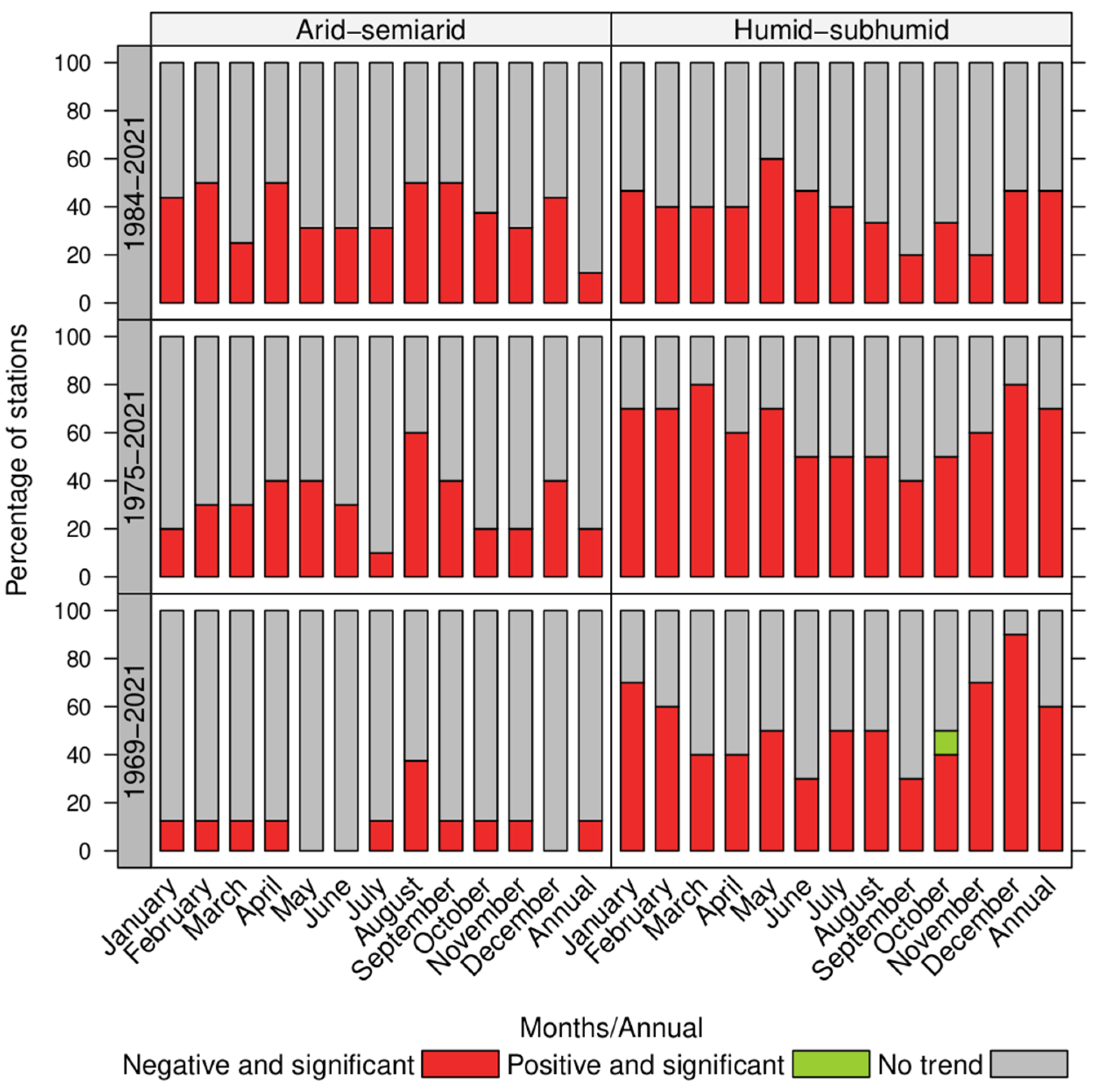
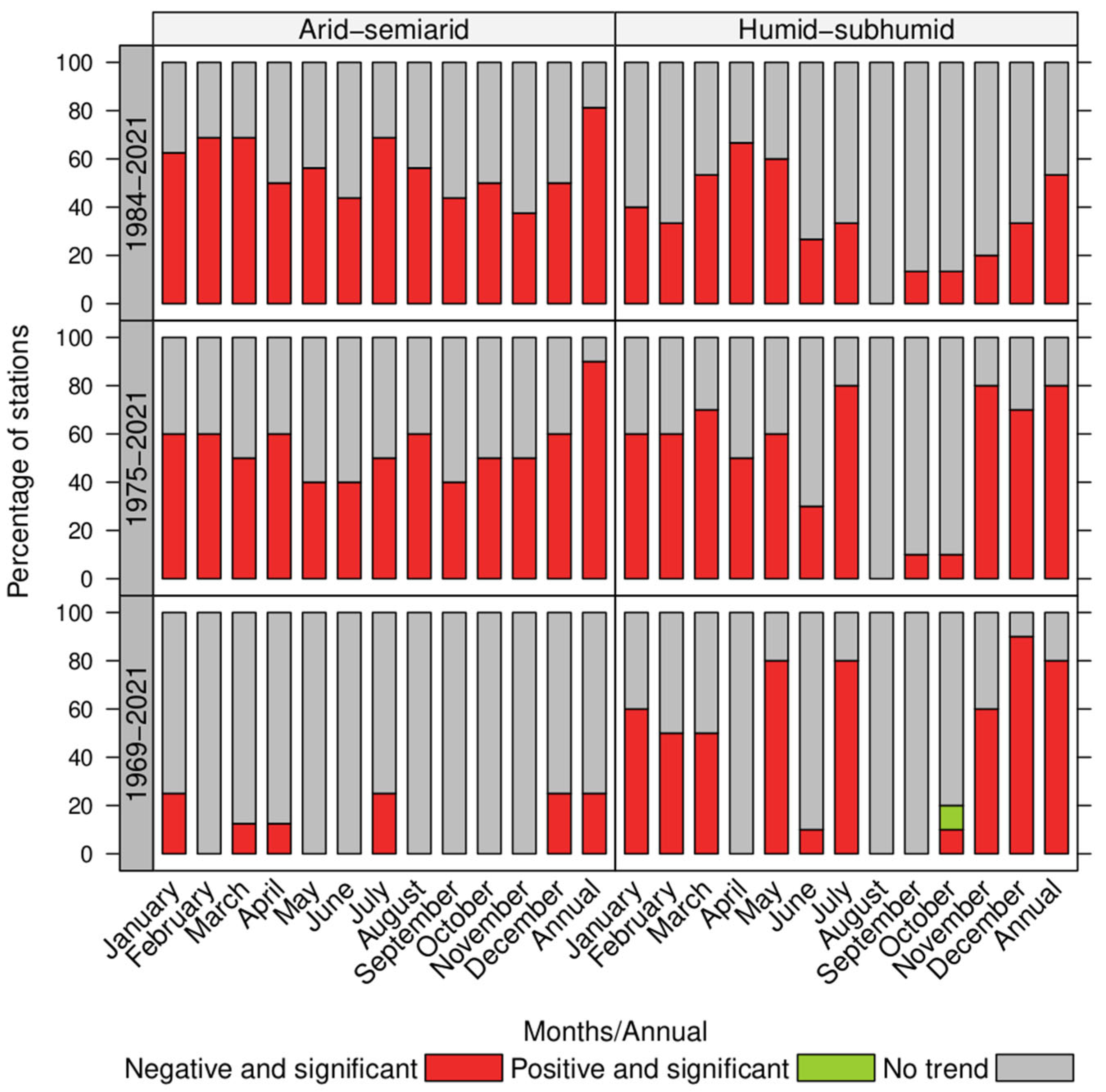
From the results at the annual scale, it is possible to observe that there was no clearly defined pattern in the behavior of the min, mean, and maximum flows in both climatic zones. However, the minimum, mean, and maximum flows in the arid–semiarid zone showed a reduction in the number of significant negative trends when the number of years of data considered increased. At the monthly scale, the flow trends in the arid–semiarid zone varied significantly as the length of the analyzed data was modified, which was not the case in the humid–subhumid zone.

To verify this, the data series were correlated with the PDO, showing that the effect of this climatic factor was more noticeable in the arid–semiarid zone, and this could explain some of the variation in the number of significant negative trends in the flow rates found for the summer months (Table 4, Table 5 and Table 6).

An important element that emerged from this study was that the results of temporal trends (in this case relative to flows) varied according to the length of the time series considered, an element that has already been highlighted by other authors such as Pellicciotti et al. [21], Valdés et al. [36] and Pizarro et al. [37]. This is highly relevant because the availability of the data series is extremely variable on a national scale and, in general, in different regions of the world. As a consequence, it is essential to consider flow time series of similar length in order to establish comparisons that are fair and unbiased from a scientific and statistical point of view. In this context, the results achieved in the arid–semiarid zone indicated that the high proportion of significant negative trends found at the monthly level was drastically reduced by incorporating a greater number of years into the series and this seemed to indicate a cyclic effect on the behaviors of the flow rates. Likewise, it is likely that the significant trends found in the 1984–2021 period were influenced by the current megadrought described in recent studies (e.g., [38]), since a decrease in precipitation has an impact on flow rates. These results are consistent with those reported by Nuñez et al. [39], who found that the flow behavior in the Coquimbo region was influenced by the (warm and cold) phases of the PDO, decreasing in the cold phase. This further supports the influence of climatic factors on the behaviors of flows, as reported by Pellicciotti et al. [21], Martínez et al. [22], and Rodgers et al. [40].

In the case of the humid–subhumid zone, the negative and significant trends that were found in the first analyzed period had a much lower value compared to the arid–semiarid zone at a monthly level. This indicates that the negative trends were much smaller in areas with a greater humidity within the country (between latitudes 34°43′ S and 38°30′ S), and this would indicate a greater stability of the maximum flows than the one reflected in the arid–semiarid zone, for the same time period analyzed. However, the stations of Ñuble in San Fabián and Biobío in Rucalhue showed decreases of approximately 10% and 30%, respectively, in decile 10 of the daily mean flow (i.e., the maximum flow values of the daily mean flow were decreasing over time) and this can also be seen in the results of the maximum flows of the humid–subhumid zone (quantile–Kendall plots in Supplementary Materials). These trends could be explained by an increase in snowmelt contributions to the flow, although the degree of their influence on the summer flow in these basins needs to be further investigated.

The results found in this study differ from those published by Novoa [19,20], where a positive trend was found in the maximum and average flows in the Claro river basin (Coquimbo region). This disparity can be explained by the different temporal resolutions and by the statistical test used to evaluate trends in the flows. Novoa [19,20] used the least-squares method to find the slope of the time series, whereas this study was based on the Mann–Kendall test, which, unlike least squares, is not affected by the presence of extreme values in the series. Moreover, Pellicciotti et al. [21] analyzed annual and monthly flow tendencies in the Aconcagua River basin (Valparaíso region; semiarid zone of the country), using the Mann–Kendall test. The authors found negative trends in both temporal resolutions, similar to the results found in this study. Additionally, Givovich [23] and Martínez et al. [22] studied mean flow tendencies (monthly and annual) in the same region, suggesting decreases in water production in the upper part of the Aconcagua river basin and positive trends in its lower portion. The latter could be explained by the outcrop of underground flows and glacial melting (as previously mentioned), although the authors did not present evidence of any of these possibilities.

From an international perspective, Rodgers et al. [40] analyzed streamflow trends in south–southeastern United States, verifying the variation as a function of the time period considered (1950–2015; 1960–2015; 1970–2015; 1980–2015; 1990–2015; and 2000–2015). Broadly speaking, the authors found that the most recent time period showed the highest number of significant negative trends. The results of this research show a similar behavior in the observed trends, particularly in the daily mean flows (see Table 3 and plots in Supplementary Materials), where the arid–semiarid zone showed a higher frequency of significant negative trends. These behavioral similarities within a climatic zone are an interesting aspect to investigate, since they were found in two different climatic zones, as described in Rodgers et al. [32] and this study. This pattern is somewhat unexpected and may be an effect of global climate change, so it is important to continue investigating the flow patterns in different climatic zones.

Based on results from this study, it is important to note that there are relevant differences between the studied basins and their geographic location, and this variability should be considered when planning and managing water resources and the territory.

One of the limitations of this study is that not all the stations have information for the three analyzed periods and, therefore, it is not possible to indicate whether in the last period, there was an increase in the negative significant trends of these stations. Similarly, another factor to consider is the impact of illegal human extractions on circulating flow rates. Pizarro et al. [33] identified that overuse is one of the main factors influencing the decrease in water supply in the Coquimbo region. Based on the above, watersheds with low intervention were selected to mitigate the impacts of this factor.

5. Conclusions

From the obtained results, it is possible to conclude that the trends of the analyzed flows (minimum, mean and maximum) were mainly negative during the analyzed periods, and this was supported by evaluating the tendency of the daily mean flows. This would suggest, as a first approximation, that the flows decreased at a monthly level. Additionally, the number of significant negative trends varied depending on the period analyzed, especially if the flows were broken down into their monthly or daily mean levels. This effect was more pronounced in the arid–semiarid zone.

A second conclusion is that it was necessary to increase the length of the data series, especially to include older time periods, because this indicated the presence of similar phenomena experienced in the past and thus reflected that similar events had previously been observed.

Finally, the correlation between the PDO and the monthly streamflow component may be a factor that explains the variation in the number of significant negative trends identified, a finding that was more clearly observed in the arid–semiarid zone and during summer months. However, further research is needed to quantify the influence of each factor on streamflow trends, and it would be interesting to study temporal changes in the magnitude of the trends. This could potentially offer a more insightful perspective that goes further than just testing for the presence or absence of trends, but also its associated dynamics and progressive attributes.

References

1. Core Writing Team; Pachauri, R.K.; Meyer, L.A. (Eds.) IPCC Climate Change 2014: Synthesis Report. In Contribution of Working Groups I, II and III to the Fifth Assessment Report of the Intergovernmental Panel on Climate Change; IPCC: Geneva, Switzerland, 2014; p. 151. [Google Scholar]
2. Ji, F.; Wu, Z.; Huang, J.; Chassignet, E.P. Evolution of Land Surface Air Temperature Trend. Nat. Clim. Chang. 2014, 4, 462–466. [Google Scholar] [CrossRef]
3. Karl, T.R.; Arguez, A.; Huang, B.; Lawrimore, J.H.; McMahon, J.R.; Menne, M.J.; Peterson, T.C.; Vose, R.S.; Zhang, H.-M. Possible Artifacts of Data Biases in the Recent Global Surface Warming Hiatus. Science 2015, 348, 1469–1472. [Google Scholar] [CrossRef] [PubMed] [Green Version]
4. Pizarro, R.; Balocchi, F.; Vera, M.; Aguilera, A.; Morales, C.; Valdés, R.; Sangüesa, C.; Vallejos, C.; Fuentes, R.; Abarza, A.; et al. Influencia del Cambio Climático en el Comportamiento de los Caudales Máximos en la Zona Mediterránea de Chile. Tecnol. Cienc. Agua 2013, 4, 5–19. [Google Scholar]
5. Fuenzalida, H.; Villagrán, C.; Bernal, P.; Fuentes, E.; Santibáñez, F.; Peña, H.; Montesino, V.; Hajek, E.; Rutllant, J. Cambio Climático Global y Eventuales Procesos en Chile. Rev. Ambiente Desarro. 1989, 5, 37–42. [Google Scholar]
6. Ivanova, Y.; Corredor, J. Evaluación de la Sensibilidad de los Caudales Máximos de Diseño Ante la Influencia del Cambio Climático. Av. Recur. Hidráulicos 2006, 13, 89–98. [Google Scholar]
7. Waylen, P.; Woo, M. Prediction of Annual Floods Generated by Mixed Processes. Water Resour. Res. 1982, 18, 1283–1286. [Google Scholar] [CrossRef]
8. Whitaker, A.; Alila, Y.; Beckers, J.; Toews, D. Evaluating Peak Flow Sensitivity to Clear-Cutting in Different Elevation Bands of a Snowmelt-Dominated Mountainous Catchment: Clear-Cutting and Snowmelt Peak Flows. Water Resour. Res. 2002, 38, 11-1–11-17. [Google Scholar] [CrossRef]
9. Carrasco, J.F.; Casassa, G.; Quintana, J. Changes of the 0 °C Isotherm and the Equilibrium Line Altitude in Central Chile during the Last Quarter of the 20th Century/Changements de L’isotherme 0 °C et de la Ligne D’équilibre des Neiges Dans le Chili Central Durant le Dernier Quart du 20ème Siècle. Hydrol. Sci. J. 2005, 50, 11. [Google Scholar] [CrossRef]
10. Carrasco, J.F.; Osorio, R.; Casassa, G. Secular Trend of the Equilibrium-Line Altitude on the Western Side of the Southern Andes, Derived from Radiosonde and Surface Observations. J. Glaciol. 2008, 54, 538–550. [Google Scholar] [CrossRef] [Green Version]
11. Torres, H.; Brenning, A.; García, J.-L. Balance de Masa del Glaciar Cubierto del Pirámide (Chile Central, 33°S) Entre 1965 y 2000 Aplicando Métodos Geodésicos. Rev. Geogr. Espac. 2013, 3, 11. [Google Scholar] [CrossRef]
12. Rosenbluth, B.; Fuenzalida, H.; Aceituno, P. Recent Temperatura Variations in Southern South America. Int. J. Climatol. 1997, 17, 67–85. [Google Scholar] [CrossRef]
13. Ollero, A. El Curso Medio del Ebro: Geomorfología Fluvial, Ecogeografia y Riesgos; Consejo de Protección de la Naturaleza de Aragón: Zaragoza, Spain, 1996; ISBN 978-84-920441-4-6. [Google Scholar]
14. Aparicio, F. Fundamentos de Hidrología de Superficie, 11th ed.; Limusa: Mexico City, Mexico, 1997. [Google Scholar]
15. Chow, V.T.; Maidment, D.; Mays, L. Hidrología Aplicada; McGraw-Hill: Bogotá, Columbia, 2000; ISBN 978-958-600-171-7. [Google Scholar]
16. Vergara, M.; Ellis, E.; Cruz, J.; Alarcón, L.; Galván, U. La Conceptualización de las Inundaciones y la Percepción del Riesgo Ambiental. Política Cult. 2011, 36, 45–69. [Google Scholar]
17. Rojas, O.; Mardones, M.; Arumí, J.L.; Aguayo, M. Una Revisión de Inundaciones Fluviales en Chile, Período 1574–2012: Causas, Recurrencia y Efectos Geográficos. Rev. Geogr. Norte Gd. 2014, 57, 177–192. [Google Scholar] [CrossRef] [Green Version]
18. Paoli, C.U.; Cacik, P.A.; Bolzicco, J.E. Análisis de Riesgo Conjunto en la Determinación de Crecidas de Proyecto de Regímenes Complejos. Ing. Agua 1998, 5, 13–22. [Google Scholar] [CrossRef] [Green Version]
19. Novoa, J.; Castillo, R.; Viada, J. Tendencia de Cambio Climático Mediante Análisis de Caudales Naturales: Cuenca del Río Claro (Chile Semiárido). An. Soc. Chil. Cienc. Geográficas 1996, 47–56. [Google Scholar]
20. Novoa, J.; Robles, M.; Castillo, R.; López, D. Tendencias Potenciales de Riesgos Morfodinámicos Mediante Interpretación de Caudales Máximos IV Región de Coquimbo-Chile Semiárido. In Proceedings of the VI Congreso Internacional de Ciencias de la Tierra Chile, Santiago, Chile, 7–11 August 2000. [Google Scholar]
21. Pellicciotti, F.; Burlando, P.; Van Vliet, K. Recent Trends in Precipitation and Streamflow in the Aconcagua River Basin, Central Chile. In Proceedings of the Glacier Mass Balance Changes and Meltwater Discharge; IAHS Press: Foz de Iguazú, Brazil, 2007; Volume 318, pp. 17–38. [Google Scholar]
22. Martínez, C.; Fernández, A.; Rubio, P. Caudales y Variabilidad Climática en Una Cuenca de Latitudes Medias en Sudamérica: Río Aconcagua, Chile Central (33°S). Boletín Asoc. Geógrafos Españoles 2012, 58, 227–248. [Google Scholar] [CrossRef] [Green Version]
23. Givovich, W. Derretimiento de las Nieves y Recursos Hídricos de la Zona Centro-Norte de Chile. Rev. Ambiente Desarro. 2006, 22, 58–67. [Google Scholar]
24. Souvignet, M.; Oyarzún, R.; Verbist, K.M.J.; Gaese, H.; Heinrich, J. Hydro-Meteorological Trends in Semi-Arid North-Central Chile (29–32°S): Water Resources Implications for a Fragile Andean Region. Hydrol. Sci. J. 2012, 57, 479–495. [Google Scholar] [CrossRef] [Green Version]
25. Kottek, M.; Grieser, J.; Beck, C.; Rudolf, B.; Rubel, F. World Map of the Köppen-Geiger Climate Classification Updated. Meteorol. Z. 2006, 15, 259–263. [Google Scholar] [CrossRef]
26. Sarricolea, P.; Herrera-Ossandon, M.; Meseguer-Ruiz, Ó. Climatic Regionalisation of Continental Chile. J. Maps 2017, 13, 66–73. [Google Scholar] [CrossRef] [Green Version]
27. Mann, H.B. Nonparametric Tests Against Trend. Econometrica 1945, 13, 245. [Google Scholar] [CrossRef]
28. Kendall, M. Rank Correlation Methods, 4th ed.; Charles Griffin: London, UK, 1975. [Google Scholar]
29. Hussain, M.; Mahmud, I. PyMannKendall: A Python Package for Non Parametric Mann Kendall Family of Trend Tests. Open Source Softw. 2019, 4, 1556. [Google Scholar] [CrossRef]
30. Benjamini, Y.; Hochberg, Y. Controlling the False Discovery Rate: A Practical and Powerful Approach to Multiple Testing. J. R. Stat. Soc. Ser. B 1995, 57, 289–300. [Google Scholar] [CrossRef]
31. Narum, S.R. Beyond Bonferroni: Less Conservative Analyses for Conservation Genetics. Conserv. Genet. 2006, 7, 783–787. [Google Scholar] [CrossRef]
32. Sen, P.K. Estimates of the Regression Coefficient Based on Kendall’s Tau. J. Am. Stat. Assoc. 1968, 63, 1379–1389. [Google Scholar] [CrossRef]
33. Lins, H.F.; Slack, J.R. Streamflow Trends in the United States. Geophys. Res. Lett. 1999, 26, 227–230. [Google Scholar] [CrossRef] [Green Version]
34. Choquette, A.F.; Hirsch, R.M.; Murphy, J.C.; Johnson, L.T.; Confesor, R.B. Tracking Changes in Nutrient Delivery to Western Lake Erie: Approaches to Compensate for Variability and Trends in Streamflow. J. Great Lakes Res. 2019, 45, 21–39. [Google Scholar] [CrossRef]
35. Bhaskar, A.S.; Hopkins, K.G.; Smith, B.K.; Stephens, T.A.; Miller, A.J. Hydrologic Signals and Surprises in U.S. Streamflow Records during Urbanization. Water Resour. Res. 2020, 56, e2019WR027039. [Google Scholar] [CrossRef]
36. Valdés-Pineda, R.; Pizarro, R.; García-Chevesich, P.; Valdés, J.B.; Olivares, C.; Vera, M.; Balocchi, F.; Pérez, F.; Vallejos, C.; Fuentes, R.; et al. Water Governance in Chile: Availability, Management and Climate Change. J. Hydrol. 2014, 519, 2538–2567. [Google Scholar] [CrossRef]
37. Pizarro, R.; García-Chevesich, P.; Balocchi, F.; Pino, J.; Ibáñez, A.; Sangüesa, C.; Vallejos, C.; Mendoza, R.; Ingram, B.; Sharp, J.O. Comparative Analysis of Annual and Monthly Peak Flow Tendencies, Considering Two Periods in North-Central Chile. Tecnol. Cienc. Agua 2022, 13, 73–100. [Google Scholar] [CrossRef]
38. Garreaud, R.D.; Boisier, J.P.; Rondanelli, R.; Montecinos, A.; Sepúlveda, H.H.; Veloso-Aguila, D. The Central Chile Mega Drought (2010–2018): A Climate Dynamics Perspective. Int. J. Climatol. 2020, 40, 421–439. [Google Scholar] [CrossRef]
39. Núñez, J.; Rivera, D.; Oyarzún, R.; Arumí, J.L. Influence of Pacific Ocean Multidecadal Variability on the Distributional Properties of Hydrological Variables in North-Central Chile. J. Hydrol. 2013, 501, 227–240. [Google Scholar] [CrossRef]
40. Rodgers, K.; Roland, V.; Hoos, A.; Crowley-Ornelas, E.; Knight, R. An Analysis of Streamflow Trends in the Southern and Southeastern US from 1950–2015. Water 2020, 12, 3345. [Google Scholar] [CrossRef]
Figure 1. Distribution of fluviometric stations and climate types within the study area. Our own work using data from Sarricolea et al. [26].
Hydrology 10 00144 g001
Figure 2. Summary of temporal analysis for minimum streamflows, using the Mann–Kendall method.
Hydrology 10 00144 g002
Figure 3. Summary of temporal analysis for mean streamflows, using the Mann–Kendall method.
Hydrology 10 00144 g003
Figure 4. Summary of temporal analysis for maximum streamflows, using the Mann–Kendall method.
Hydrology 10 00144 g004