4.1. Annual Rainfall, Streamflow, ROC, ET, and PET
Annual rainfall data are summarized in
Table 3 for the 17-year (2005–2021) study period. Rainfall varied from as low as 994 mm in 2007 to as high as 2243 mm in 2015, with an average of 1470 mm and a COV of 0.23. This COV is greater than the 0.18 observed during 13-year historic 1964–1976 period reported by Amatya and Trettin [
85], likely due to low and high extremes that were 27% lower and 64% higher, respectively, than the historic average of 1320 mm for the study site as well as the long-term (1946–2008) average of 1370 mm for the nearby the SEF headquarters rain gauge [
27]. The highest rainfall in 2015 was an indirect result of Hurricane Joaquin (which stayed in the ocean off the coast) leading to extremely high precipitation that resulted in 470 mm in a 2-day (3–4 October) period, which was close to the 440 mm recorded at Charleston airport [
86]. Eleven out of the seventeen years, particularly from 2013 to 2020, yielded higher than long-term average rainfall.
The estimated annual Priestley–Taylor (P-T)-based PET ranged from 1116 mm in 2009 to as high as 1350 mm in 2019, with an average of 1255 mm (
Table 3), similar to the water year-based PET of 1254 mm which also had a COV of 0.05 (
Appendix A Table A2). This average was about 10% higher than the average of 1137 mm for the 1946–2008 period obtained by Dai et al. [
27] and about 5% higher than the 1194 mm average for the 2011–2021 period, both calculated using the Hargreaves–Samani PET method. In addition, the P-T average of 1255 mm was 16% higher than 1079 mm average obtained by Amatya and Trettin [
85] using the Thornthwaite PET method for the 1964–1976 period using data from the SEF weather station. One possible reason for the higher P-T-based PET may also be due to omission of daily soil heat flux in the energy component and inherent differences in the PET methods compared here [
63,
87]. It may also be explained by differences in the in recording periods.
Annual streamflow varied from as low as 23 mm in 2012 to as high as 1517 mm in the extremely wet year of 2015 (
Table 3;
Figure 2). Note that the relatively dry year of 2012, preceded by an even drier year in 2011, resulted in the lowest flow (23 mm) and lowest ROC (0.02) for the entire period of record. Interestingly, 2007 had a similar dry period yet yielded a higher flow and ROC of 94 mm and 0.09, respectively, compared to 2012 despite 2007 having the lowest rainfall on record. We presume this was due to wetter antecedent conditions in 2006 compared to 2011. In addition, the potential energy demands of 2599 mm PET in 2011–2012 were also higher than the 2510 mm recorded for 2006–2007. This potentially resulted in a higher total 2 year ET of 2080 mm with increased storage compared to only 1903 mm for 2006–2007, with a wetter initial year of 2006 compared to the initial year of 2011, yielding a 133 mm lower flow in 2011–2012 (
Table 3). Notably, the water year-based ET of 1023 mm in 2007 (
Appendix A Table A2) was 123 mm higher than the calendar year ET of 900 mm (
Table 3). The same is true for the water year-based ET estimation for 2011 and 2012 both of which have higher ET than the corresponding calendar year values (
Table 3). On an annual basis, the water year-basis ET may be more realistic because it minimizes the storage effects due to ET when its demand is the lowest in April.
Average annual flow response to the rainfall, as shown by the ROC of 0.24, ranged from 0.02 to 0.68 in 2015 due to the extreme rainfall event. This average is consistent with the average from the water year-based value (
Appendix A Table A2) of 0.24 reported for the 1964–1976 period with only 1320 mm rainfall [
85] as well as for the small 155 ha WS77 watershed, with similar management practices, for the 2011–2019 period but with slightly higher average (1496 mm) rainfall [
25]. Hazardous fuel treatment for understory removal on about 93% of the watershed (
Appendix A Figure A2) in the dry year of 2012 might not have affected flows due to the very dry conditions. This is consistent with the authors of [
60] who noted that these systems (whether treated or untreated) may respond similarly in extreme wet and/or dry conditions. A double mass curve analysis using cumulative annual flow versus rainfall (not shown) indicates some rising flow trend starting in 2015 as also observed in
Figure 2.
Average annual ET of 1077 mm for this period (
Table 3) (similar to the water-year average ET of 1079 mm;
Appendix A Table A2) was 9.6% higher than the 983 mm obtained for the relatively drier historic 1964–1976 period [
84], indicating that the system is moisture limited [
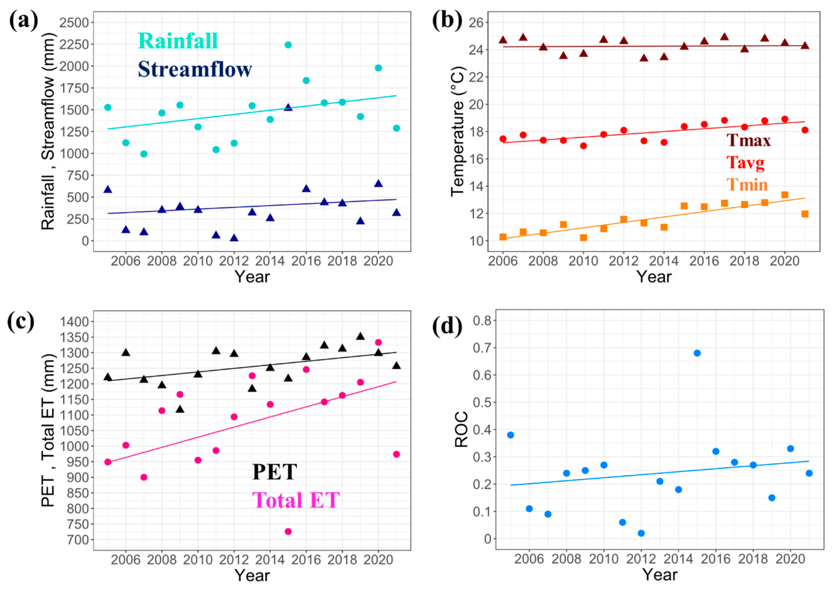
88]. This was mainly attributed to a higher but insignificant rising trend of rainfall (
Figure 3a;
Table 4 shown below), providing increased recharge (soil moisture), as well as significantly increasing temperature and PET (
Figure 3b,c). The annual ET/Rain ratios varied from 0.32 in the wettest year of 2015 to as high as 0.98 in 2012, with an average of 0.76 (same for the water-year;
Appendix A Table A2). This value indicates that about 76% of annual rainfall, on average, is lost to ET, assuming no storage and loss to groundwater. This also indicates that, despite abundant moisture from the rainfall in 2015, the available energy of 1216 mm PET might have limited additional ET loss in this year as opposed to the ET loss of 1094 mm in 2012, close to the rainfall amount, with abundant energy of 1295 mm PET (
Table 3). The ET/PET ratio varied from 0.74 in the year 2007 with the lowest rainfall to as high as 1.05 (e.g., ET > PET) in 2009, with an average of 0.86 (
Table 3). These data show that, given the moisture and energy available to evaporate it, the percentage increase in annual ET loss can likely be higher than the percentage loss as drainage to streamflow.
Annual ET, calculated here as the difference between total rainfall (not throughfall after canopy interception) and streamflow assuming no other losses, can be expected to be higher than the grass-reference PET during wet years due to higher seasonal evaporative losses from rainfall intercepted by the forest canopy [
89,
90]. In addition, long-term annual ET may be close to the PET of these forested wetlands with relatively abundant moisture [
25,
32,
89,
91]. These results are important indicators for understanding pre-development hydrology and stormwater management practices on these forest lands.
4.2. Trends in Annual Rainfall, Temperature, Streamflow, Runoff Coefficient (ROC), PET, and ET
Annual rainfall including the year of 2015 with or without the extreme wet month of October both showed increasing, but not significant (
p = 0.11 and
p = 0.12, respectively), trends (
Figure 3a;
Table 4). This is consistent with Mizzell et al. [
92] who observed gauges across the State of South Carolina as well as the authors of [
27] who also found a slight increase but not a significant change in annual rainfall observed at the Santee Experimental Forest gauge over the period of 1946–2008 [
27]. Increasing annual trends (Sens’s slope) are also exhibited by minimum, average, and maximum temperatures (
Figure 3b), with the minimum and average showing a statistically significant trend (
p-value < 0.05) but not the maximum temperature (
p = 0.92) (
Table 4). The increasing trend in average temperature is consistent with [
27] who also reported a steady increase in temperature at the SEF station during the 1981–2008 and Mizzell et al. [
92] who also reported a steady increase in temperatures across the state of SC since the 1970s. Both the estimated
p-T-based annual PET and total ET (rainfall–streamflow) show significant increasing trends, with
p = 0.003 and
p = 0.04, respectively (
Table 4). Annual streamflow reflected the temporal pattern of the rainfall, also yielding a non-significant (
p = 0.46) trend for the same 17-year period (
Figure 3a). The annual ROC, response of streamflow to rainfall, exhibited an increasing, but also non-significant (
p = 0.43), linear trend (
Figure 3d similar to the streamflow (
Figure 3a).
The effects of a significant increase in temperature (
Figure 3b) and increasing (
p = 0.03) trend in PET (
Figure 3c) were likely offset by slightly increasing rainfall (
Figure 3a), resulting in non-significant trends in streamflow (
p = 0.46) and ROC (
p = 0.43). This is similar to Dai et al. [
27]’s inference that an increase in temperature will further reduce streamflow due to an increase in ET demands if the increased demand is not offset by additional precipitation. Although some of these results are also consistent with those reported for a long-term pine plantation study site in North Carolina [
93], a longer period of data may be needed for a definitive conclusion about the trends at this site. Nonetheless, this information on recent trends for these hydrological variables may be of interest to forest managers, engineers, and land use planners.
4.3. Monthly Rainfall and Streamflow
Measured monthly streamflow responded to corresponding rainfall as shown in
Figure 4 for 2005 to 2021 period. The plot clearly indicates that the study period yielded more wet months, exceeding 200 mm rain, starting in 2014 (21 months) compared to the previous 9-year period (15 months), with extended no flow months, particularly in 2006–2007 and 2011–2012. Those four years yielded very low annual ROC values as discussed above. The wet year of 2015 had 726 mm of flow during October due to an indirect effect of Hurricane Joaquin [
94]. Other high rainfall months were October 2016 (316 mm; Hurricane Matthew) and August 2020 (429 mm; Hurricane Isaias). Based on the National Weather Service
https://www.weather.gov/chs/TChistory (accessed on 20 February 2024), from 1950 to 2018, more tropical cyclones occurred during “cool” El Nino-Southern Oscillation (ENSO) conditions (i.e., La Nina) compared to “warm” ENSO conditions (i.e., El Nino), with major hurricanes during 2019–2021 under La Nina or neutral ENSO conditions
https://www.washingtonpost.com/weather/2022/04/27/la-nina-triple-hurricanes-tornadoes/ (accessed on 20 February 2024). Some months with extended no flows occurred in relatively dry years of 2006, 2007, 2011, and 2012 with below average rainfall (
Figure 4). The mean monthly ROC of 0.24 is consistent with that of 0.22 obtained for the annual period (
Table 1).
On the water year basis (analyzed for 2006–2021), the growing season’s (April–October) ROC of 0.30 was 50% higher than that (0.20) of the dormant season (November–March) despite nearly 71% (1041 mm) of the average total rainfall (1469 mm) being recorded in the growing season (
Appendix A Table A3). This was likely due to the growing season average ET of 795 mm, which was 179% higher than the dormant season average (285 mm) with its reduced ET demands. The growing season ET was 73.6% of the average annual ET of 1079 mm, consistent with similar other regional studies [
26,
90].
4.4. Daily Rainfall Frequency Duration
Daily rainfall frequency duration for the 2005–2021 period (6209 days) is shown in
Figure 5a. Daily rainfall exceeded 60 mm and 12.5 mm for 1% (62 days) and 10% of the time, respectively. The data show that 24 h rainfall exceeded 100 mm or more 0.2% of the time (12 days) (
Figure 5b), most of which occurred since 2015. Most of these large events were associated with tropical storm events (
Figure 5a), with a 24 h total of 271 mm and 471 mm over two days on 3–4 October of 2015 (Hurricane Joaquin), 219 mm on 8 October 2016 (Hurricane Matthew), and 206 mm on 5 September 2019 (Hurricane Dorian). The highest recorded total rain in October of 2015 was consistent with Mizzell et al. [
86] who reported that all time precipitation records were set across the coastal plain, with totals ranging from 254 mm to over 660 mm.
The data in
Figure 5b show the number of daily precipitation events of various sizes recorded during the study period. The number of storm events is increasing, but not significant, for all rain sizes; the steepest trend was for 26–50 mm size storms, with the largest number (19) in 2015 followed by (17) in 2017.
However, how these storm event rainfall sizes are translated into storm runoff event dynamics are yet to be examined. For example, using the rainfall–runoff data from this site for the 1964–1976 historic period, La Torres Torre [
43] found that runoff–rainfall ratios were greater for wet (winter–spring) periods compared to dry (summer-fall) periods and runoff response was related to antecedent soil moisture conditions for wet and dry conditions. The second part of the runoff response was, however, partially studied by Epps et al. [
28] for streamflow and direct runoff as response to storm events response linking them also to position of the pre-event water table position. In addition, recently Amatya et al. [
52] linked the direct runoff response to pre-event water table and a soil profile saturation parameter by using data from first-order low-gradient coastal catchments including two nested ones from this study site.
4.5. Daily Flow Duration Frequency Curves
Daily flow duration curves are presented in
Figure 6 for the 2005–2021 period since regeneration of forest stands 15 years after Hurricane Hugo impacted the area in 1989 [
1]. The smaller plot on the right of
Figure 6 shows the 1% to 100% exceedance probability behavior for stream flow (discharge). The data showed that the daily flow exceeded zero discharge 75.7% of the time, compared to the value of 79% of the time observed by Amatya and Radecki-Pawlik [
95] using 13 years (1964–1976) of historic data from this watershed. However, no significant trend in annual outflows was observed (
Figure 3a). The frequency plot also shows that this third-order coastal watershed had no flow for about a quarter of the year, on average. Flows of 10.0 mm day
−1 or higher occurred <1.21% of the time, with the highest daily flow of 256.8 mm on 5 October 2015 by 242 mm on 4 October, 205 mm on 6 October, and 116.7 mm on 7 October in 2015, as a result of nearly 500 mm rain during 3–4 October (
Figure 5a). Similarly, Hurricane Matthew produced 96.2 mm of flow on 8 October 2016, as a result of a 200 mm storm total. This trend is consistent with other studies reporting potentially higher and more intensive storms and peak flows [
27,
93]. Flows less than 5.0 mm day
−1 occurred 95.7% of time, most of which (59%) occurred during winter (December–February) and spring (March–May) periods. Flows larger than 15.0 mm day
−1 were observed mostly during the fall (September-November) season. These results have implications in managing infrastructure for flow for flood resilience as well as in planning for ecological restorations [
96,
97].
An analysis of daily baseflow computed using an automatic digital filtering technique for the 2006–2021 period provided a mean daily baseflow of 0.22 m
3 s
−1, which is about 35% of the measured mean daily runoff of 0.634 m
3 s
−1. Using a baseline separation method on Florida coastal watersheds, La Torre Torres et al. [
44] found a baseflow of 23%, on average, of total runoff for 41 storm events analyzed from this study watershed for the 1964–1976 historic period. This average was lower than the 47% reported by Morrison [
57] using a different partitioning method for 15 events of the recent 2011–2015 period. These results show a wide variation in base flow estimates depending upon the analyzed period, temporal scale, and method of partitioning.
4.6. Daily Flow Rate Frequencies for Dry, Wet, and Normal Years
Daily flow rate duration curves for two relatively dry (2007, 2012), two relatively normal (2008, 2013), and two relatively wet (2015, 2020) years in the 2006–2021 period are shown in
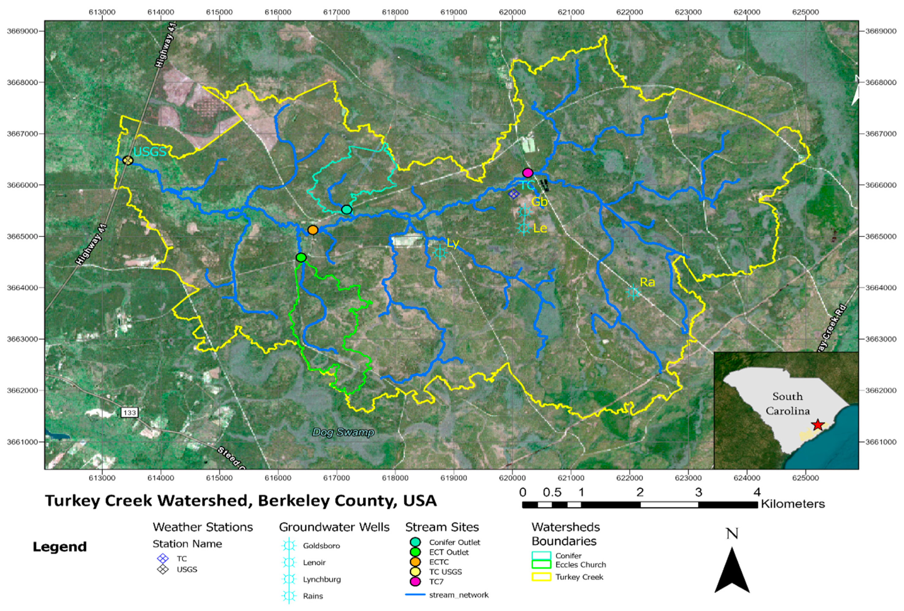
Figure 7. During dry conditions, both curves for 2007 and 2012 are plotted lower compared to curves for normal and wet years. The flow rates for all ranges of frequency are lowest and have small variability compared to the wet and normal years. The small amount of variability in flow during dry years is caused by higher water storage and a lower water table (as shown below under the Water Table section) in forested watersheds with high ET demand and influence of groundwater sources in total streamflow. Moreover, large areas of poorly drained Wahee soil series on the right streambank (
Figure 1) may play a dominant role in recharging stream during dry season. Flow during dry years was observed only for about 20 to 60% of analyzed period, which can have an adverse impact on stream ecosystem health potentially due to stressful conditions caused by low oxygen and concentrated chemicals. The wet years yielded the highest low flow rates, compared to normal and dry years, that are important for ecosystems to ensure optimal biodiversity of macroinventerebrates [
98,
99]. The extremely high flow rates during the wet years were caused by extreme rainfall and very shallow water table elevations causing soil saturation (
Figure 5a). Curves for normal years, showing the highest variability in flow, lie between the curves for wet and dry conditions. Compared to dry years, wet years resulted in a lower number of zero flow days (about 10 of 20% of analyzed period), with the rest yielding low flow rates, consistent with
Figure 6.
4.7. Peak Discharge versus Rainfall of Various Duration
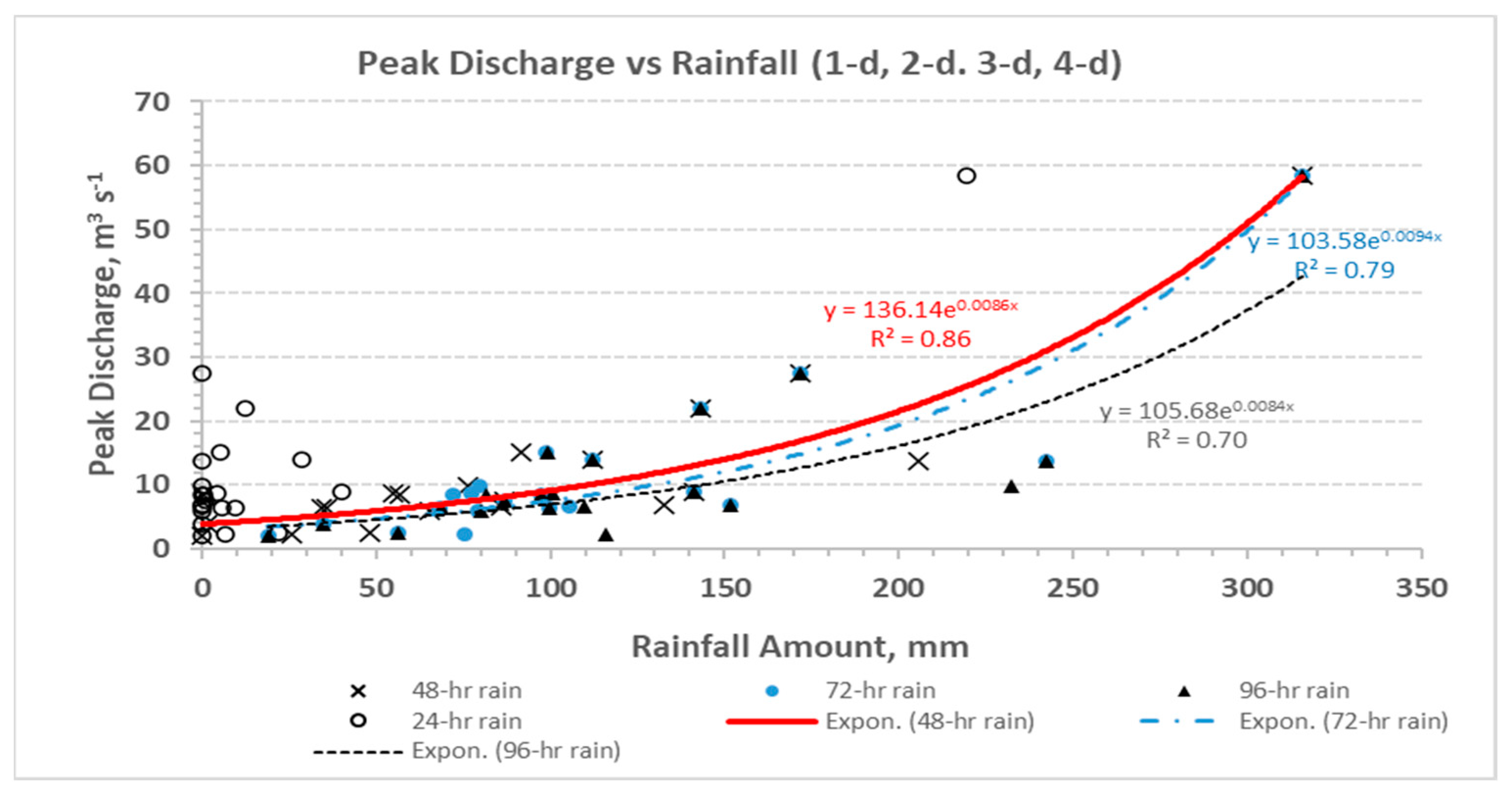
The data in
Figure 8 show fitted lines using exponential relationships for observed peak discharges with their corresponding rainfall amounts accumulated over 24, 48, 72, and 96 h durations prior to the peak discharge for the study period, except for the extremely large event of 3–5 October 2015. An exponential increase in runoff for storm events with the water table near or above the surface was reported in earlier studies for nearby watersheds [
30,
100].
Apparently, the strongest relationship of the peak discharge on this 52 km
2 watershed was found for the 48 h duration with the highest R
2 of 0.86 followed by the 72 h duration (R
2 = 0.79). Coincidentally, the USGS estimated peak discharge of approximately 158 m
3 s
−1 for that excluded October extreme event (
https://nwis.waterdata.usgs.gov/nwis/peak?site_no=02172035&agency_cd=USGS&format=html; accessed on 20 February 2024) was the result of a 48 h rainfall amount exceeding 470 mm. There was no relationship with the 24 h (daily) duration, indicating that the time of concentration (t
c) (defined as the time of flow travel from the most remote point on the watershed to its outlet) used for identifying rainfall intensity in event hydrologic models [
19,
53] for computing flood discharges for water infrastructure design on watersheds of these sizes should exceed 24 h or more. This implies an effect of a larger storm cell size yielding a longer t
c as the watershed size increases [
19]. The t
c of a near 3 h storm duration was estimated for computing design discharges for a much smaller 160 ha WS80 watershed [
11,
19] adjacent to this study site. Most large peak discharges likely resulted for events when most watershed had saturated/ponded soil conditions or near surface water table (WT) depths (25–27 October 2008; 4–6 October 2015; 8 October 2016; see the following section) possibly contributing to overland surface or shallow subsurface runoff on these low-gradient poorly drained landscape [
52].
4.8. Water Table
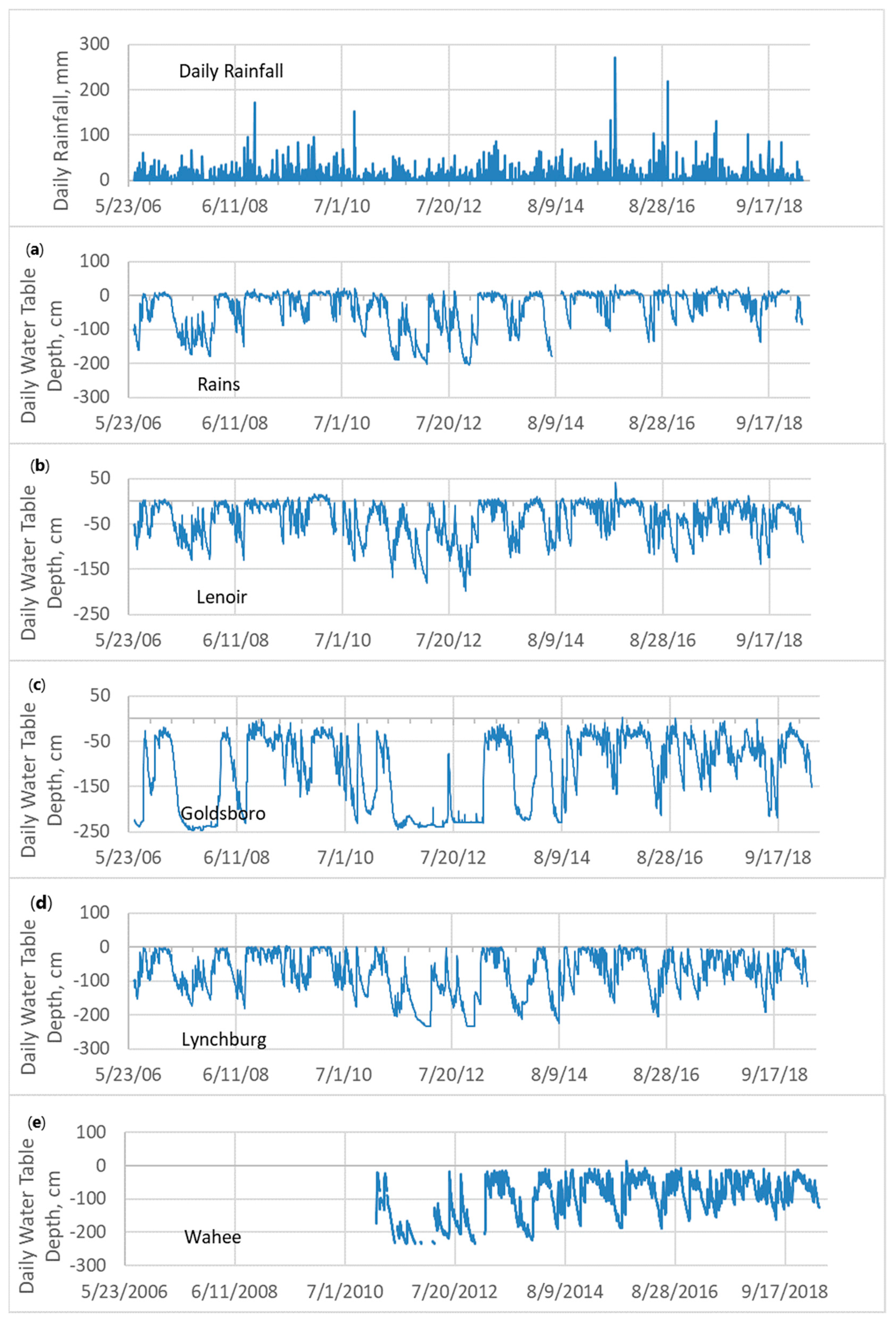
Time series data of WT dynamics from wells in four dominant soil types are presented together with daily rainfall in
Figure 9. Earlier work by Amatya et al. [
60] using data through 2016 showed no significant trends for daily water table position (
p = 0.84 for Rains; =0.28 for Lenoir; 1.00 for Goldsboro, and 0.48 for Lynchburg) at well locations on the study site. No data analysis was carried out for the Wahee well due to limited data.
The mean WT depth for that period varied from about 46 cm for the wells in Rains and Lenoir soils to 122 cm for the well in the well-drained Goldsboro soil, with WT depths of 85 cm for the well in moderately drained Lynchburg soil. A similar pattern for mean water table depths was obtained for the data extended through 2021, with a WT as deep as 2.5 m for the Goldsboro location to even surface ponding of as much as 46 cm for the Lenoir soil during the extreme event of 3–4 October 2015, when all the other wells also responded with a WT at the surface [
94]. However, the duration of saturation and ponding depended on the soil type, as shown by Williams and Amatya [
101] who referred to soil drainage class and soil taxonomy in their analysis. Any additional rainfall during pre-saturated conditions may result in localized as well as watershed-wide overland runoff [
52] with a potential for large peak discharge flooding the area, as observed during the 3–4 October 2015 extreme event discussed above.
In a recent storm-event modeling study, Amatya et al. [
52] used data from two catchments within the Turkey Creek watershed, and a third adjacent small watershed (WS80), each <210 ha in area. Modeling results showed that a threshold rainfall amount of 110 mm generated shallow surface runoff in addition to shallow subsurface flow due to saturation-excess conditions. The pre-event water table elevation with a soil saturation coefficient (α) model parameter described the saturated depth necessary to partition the storm event volume into overland surface and subsurface runoff. Variability in event runoff was attributed to seasonal trends in water table elevation fluctuation as regulated by soil moisture and evapotranspiration [
28,
44,
102]. During the extreme rainfall events of 3–4 October 2015, and 8 October 2016, water tables across the watershed responded similarly, rising to the surface with sustained ponding in some well locations, likely contributing to surface runoff and peak discharge. Note that the water table response (
Figure 8) shows several saturation-excess periods of varying durations, especially for the more poorly drained sites with Lenoir, Lynchburg, and Rains soil series. The extreme storm event of 3–4 October 2015 created saturated or near-saturated conditions for several months at those sites.
A comparative analysis of groundwater position data in the shallow well (screened from surface to 3 m deep) and deeper subsurface piezometer (screened at 14.5 m deep) at the same location as the water table well in the Lenoir soil (upper Turkey Creek) (
Figure 10) provided an average recharge estimate to the surficial aquifer of 114 ± 60 mm y
−1 [
51]. The main factor influencing recharge estimates was antecedent water table level, which in turn was influenced by landscape position and soil texture. The shallow water table conditions at this site support a large range of natural wetlands and create management challenges across the region [
103]. Modest changes in the position of the water table can lead to either groundwater flooding and concomitant management challenges for silvicultural activities, or to ecosystem stresses related to dry conditions in wetlands during times of below-normal precipitation or because of groundwater withdrawal.
Plots for both the water table and piezometric data in
Figure 10 indicate a possible change in the trend or a break point somewhere between 2010 and 2012. Results of Pettitt’s test for change detection for the significance level α of 0.05. are presented in
Table 5.
Analysis of Pettitt’s test using a critical value depends on the number of observations (77 and 79 values for water table and piezometer water depth in this case) in the time-series and the assumed significant level. Based on Jaiswal et al. [
104], the critical values analyzed for the 0.05 significance level were determined as 459 and 478 for the water table and piezometer data, respectively. The analysis indicated that the break point could have occurred on 9 December 2012 or 1 April 2010. However, the computed values of
U for the Pettitt test were lower than the U
crit, indicating a lack of trend and lack of break-change points in both the water table and piezometric data.
4.9. Precipitation Intensity–Duration–Frequencies and Design Flood Frequencies
Compared to the mean onsite 24 h and 48 h precipitation depths for the 2005–2021 period, the NOAA-Atlas14 values for the 1893–2002 period considerably underestimate the precipitation for the 10-, 25-, 50-, and 100-year return intervals for the same rain-gauge location (
Figure 11a,b).
As expected, the single on-site precipitation depths exhibit a wider range of uncertainty depicted by the larger confidence intervals mainly due to their relatively brief data record period. We did not use data from some other on-site gauges within its vicinity but highly recommend that this be explored in future. Similar underestimates, by 10–60% for durations ≥2 h, were observed by [
19] with errors increasing for longer return intervals when compared to estimates using data from the adjacent WS80 watershed. Based on these results, it would likely be useful to re-evaluate the hydro-geomorphologic risk analysis of culverts located within this study site, that were noted by [
20] as being vulnerable to NOAA-based 100 yr 30 min precipitation intensities.
The data in
Figure 12 show that the 2-, 5-, and 10-year design flow rates estimated by the regional USGS regression equations for the coastal plain region [
105] seem to match with those obtained using the Log Pearson Type III (LPIII) fitted flow rates for the on-site observed annual maximum peak discharge data.
The USGS regression equation derived flow rates for 25-year and longer return intervals seem to be underestimated, especially for the 100-year return interval compared to the on-site data. Like with the precipitation intensities discussed above, the larger uncertainty bands for the on-site LPIII estimates (
Figure 12) are likely due to use of the shorter recording period than the USGS methods.
In an earlier study using 13 years (1964–1976) of historic data with just the Pearson Type III model, Amatya and Radecki-Pawlik [
95] reported similar design discharges to those reported by the USGS method [
84] for return periods of ≤10-years but lower values, with underpredictions by as much as 29%, than the USGS ones for the higher return periods (
Figure 12). Results from the recent 2005–2021 period show much larger mean design flow rates than those obtained from the current USGS method updated by Feaster et al. [
105], which suggests increasing frequencies and sizes of larger peak discharges (
Figure 6 and
Figure 8), consistent with related increases in PIs and sizes (
Figure 5 and
Figure 11). These results emphasize that planners and designers should take precautionary measures while designing climate resilient stormwater and road drainage infrastructure using the published USGS regional regression equations on such watersheds.

 ,
, 


