Estimating Drainage from Forest Water Reclamation Facilities Based on Drain Gauge Measurements

Abstract

A growing human population requires sustainable solutions to regulate and dispose of municipal wastewater. Water treatment facilities in northern Idaho are permitted to apply reclaimed wastewater to forest land during the growing season at specified monthly hydraulic loading rates. We assessed the spatial and temporal variability of drainage below the rooting zone between non-irrigated (control) and irrigated (effluent) stands during the growing and dormant seasons in 2021. No drainage was observed during the two months of annual seasonal drought, but large magnitudes of drainage were recorded during the dormant season (38–94 cm), which was consistent with seasonal precipitation. The overall effect of effluent treatment on the drain gauge measurements did not differ from the controls, as effluent only increased the drainage at some facilities. The measured drainage averaged from 35 to 62 cm among facilities. We then used the drainage measurements to calibrate hydrological models (Hydrus-1D and Water Erosion Prediction Project [WEPP]) and predict the drainage in 50 measurement plots distributed evenly among five forest water reclamation facilities. As with the observed drainage, there were no statistically significant growing season differences in the predicted monthly drainage during the growing season between the effluent and control plots, suggesting the successful use of hydrologic models to support the measured drainage findings. While both models struggled to accurately predict the quantity of drainage during the dormant season, they both successfully predicted that drainage would continue through May. WEPP also successfully predicted that the treated plots began to drain in September and October following late-season irrigation at some facilities. The models showed that the prescribed crop coefficient used by the Idaho Department of Environmental Quality was adequate in avoiding drainage during the peak summer months.

1. Introduction

As human population growth produces more wastewater, it is imperative to develop environmentally sustainable and efficient water reclamation approaches. The land application of wastewater is a cost-effective and resourceful management solution for effluent reclamation following secondary treatment [1]. Wastewater simultaneously provides plant growth resources, thereby stimulating the production of conventional crops [2,3], as well as that of deciduous [4,5,6] and coniferous forests [7,8]. Wastewater applied to forest vegetation types is referred to here as forest water reclamation (FWR). There are dozens of FWR facilities permitted to operate in northern Idaho, which can enhance tree growth from 30% to over 110% [9]. Forests that are consistently water-limited during the growing season will consume the water supplied during wastewater irrigation and effectively reclaim treated effluents without environmental risk if carefully regulated.

Irrigating crops with wastewater requires compliance with irrigation scheduling guidelines. The methods used to schedule irrigation for crops include plant stress measurements, soil water measurements, and soil water balance calculations [10]. The Idaho Department of Environmental Quality (IDEQ) uses a soil water balance approach for permitting wastewater land application at facilities. An irrigation water requirement (IWR) is calculated for each month during the growing season as a function of stored soil water, soil water holding capacity, and evapotranspiration [11] multiplied by a crop coefficient. The reference crop is generally alfalfa, while the crop coefficient is the ratio of the actual crop evapotranspiration to the reference crop evapotranspiration [12]. The IDEQ recommends using a generalized crop coefficient of 0.7 for mixed conifer forests because the evapotranspiration rates for this crop are poorly characterized [13,14]. Permit-specific IWRs are calculated based on historic monthly evapotranspiration and precipitation rates and the 0.7 crop coefficient. Permits also require that the applied monthly volume of wastewater irrigation be “substantially less” than the monthly IWR [11]. Maintaining irrigation below the IWR is achieved through irrigation schedules and the incorporation of irrigation rest periods. Rest periods generally occur during weekends and after precipitation events, however, the timing and duration of rest periods are determined by facility managers [11]. The inclusion of rest periods and irrigating well below monthly IWRs are main components in the irrigation schedule guidelines for FWR facilities in Idaho.

One of the potential outcomes of irrigating above the monthly IWR is deep soil drainage. Deep soil drainage is a difficult-to-measure component of the soil water balance equation. Previous studies conducted at FWR facilities have not, to our knowledge, quantified deep soil drainage, and have instead measured individual tree water use directly [15] or modeled the water budget to determine drainage as the water added in excess of the soil water-holding capacity [16]. Birch et al. [17] evaluated the wastewater composition of streamflow, groundwater, and surface water in a coniferous forest irrigated with wastewater, but did not quantitatively assess drainage. Roygard et al. [18] measured the transpiration and runoff in isolated saplings grown in weighing lysimeters and found substantial leaching, but this is difficult to accurately scale to the stand level. It is necessary to evaluate the magnitude of drainage at these facilities because of the potential environmental risks posed by FWR. The seasonal increase in soil moisture content elevates the risk of constituent leaching, as water can rapidly percolate through soil pores and preferential flow pathways [19,20]. Measuring soil drainage rates provides flow data to quantify the occurrence of leaching in wastewater-irrigated forests, especially if the measurement approach includes intact preferential flow paths [21].

Historically, soil drainage has been measured using pan lysimeters. The design of pan lysimeters encourages water to divert around the device and reduces its efficiency by almost 90% [22]. Passive-wick lysimeters also measure soil drainage. An intact soil column contained within a control tube resides directly above a wick. The wicking material holds a fixed tension at the base of the soil column and pulls water into the reservoir below. The soil at the base of the soil column remains in an unsaturated state and through-flow is not restricted [23]. The inclusion of the wick allows the device to capture more drainage than pan lysimeters, with the intent of making these passive-wick lysimeters more accurate in quantifying deep soil drainage [24]. When compared to other lysimeter types, studies show that passive-wick lysimeters record greater drainage during high-precipitation events [25].

In this study, we used multiple drain gauges to measure drainage, parameterize hydrologic models, and predict the potential drainage occurring at five north Idaho FWR facilities. These facilities have been irrigating forests with secondary-treated wastewater for various time periods, with the earliest facility established in 1978 and the latest facility established in 2013. The main objectives of this study were to (1) measure the rate and spatial variability of drainage within and across these facilities that are annually irrigating forests with wastewater, and (2) assess the utility of hydrologic models (Hydrus-1D and Water Erosion Prediction Project [WEPP]) to predict drainage in both non-treated control stands and those receiving wastewater irrigation. We hypothesized that the drainage measured from drain gauges would not be significantly different between irrigated and non-irrigated plots within facilities. We also hypothesized that forests can assimilate the permitted irrigation rates during the growing season when applying the crop coefficient of 0.7 recommended by the IDEQ handbook.

2. Materials and Methods

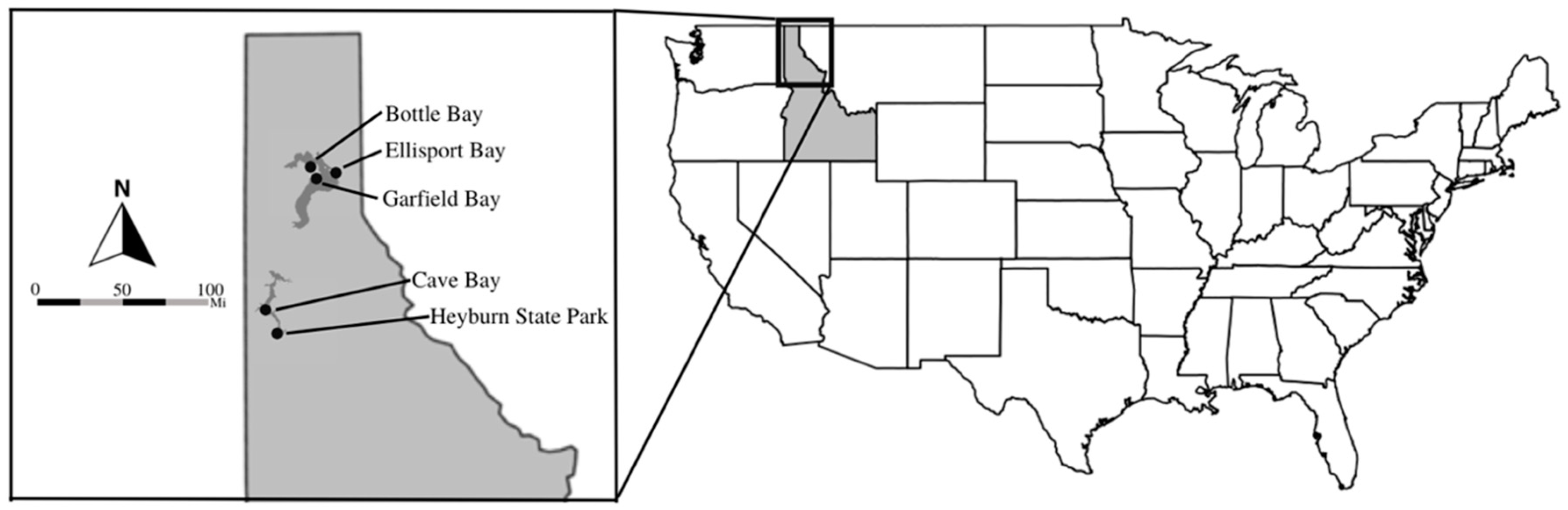
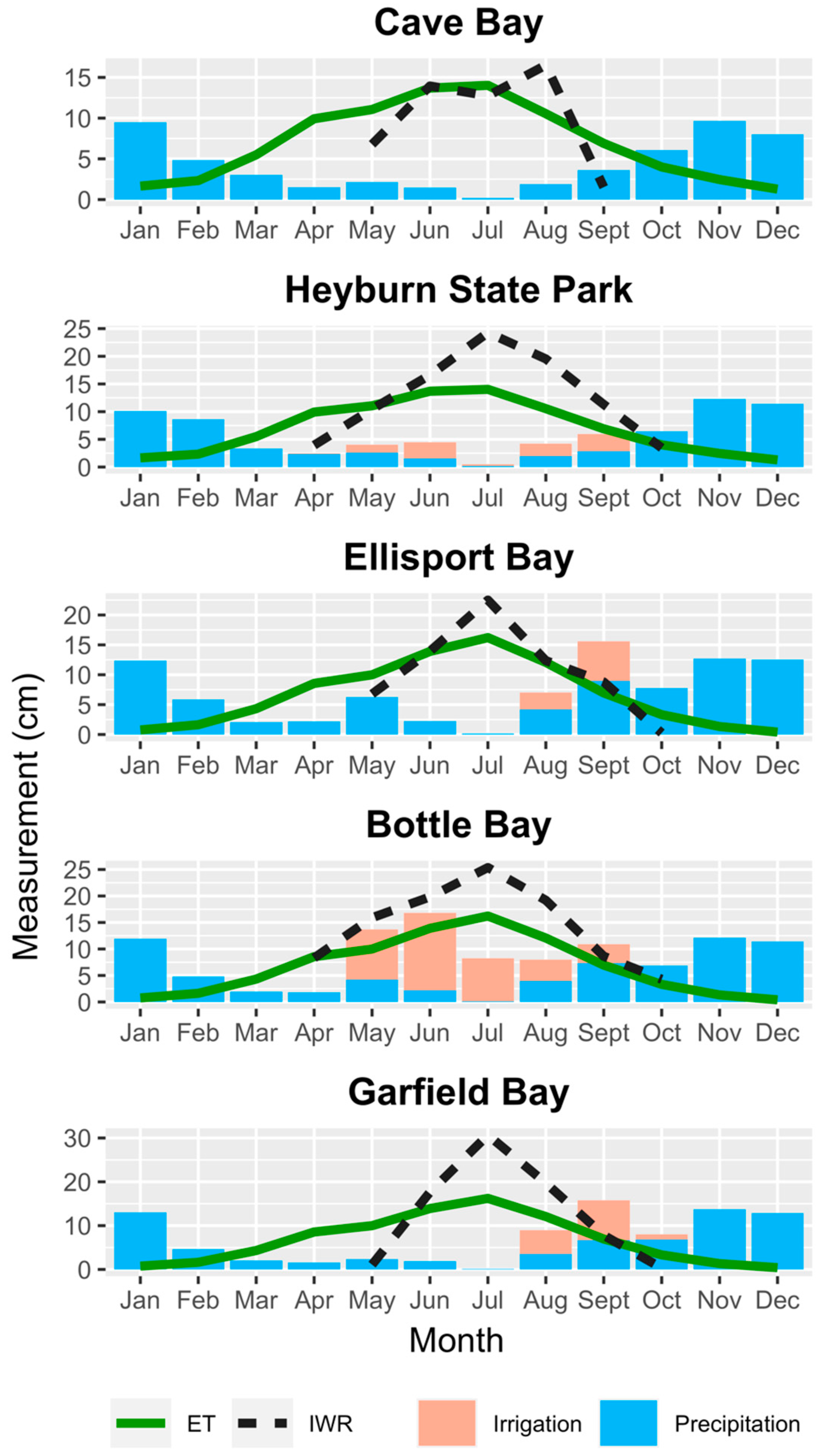
2.1. Study Area

The FWR facilities involved in this study were in northern Idaho (Figure 1,

Table 1. Location, establishment, and climate information for study facilities.

Facility	Location	Establishment Date	Mean Annual Precipitation (cm)	MAT (°C)	Mean Maximum Temperature (°C)	Mean Minimum Temperature (°C)
Cave Bay	47.46, −116.88	2013	53.4	8.4	19.6	−5.1
Heyburn State Park	47.34, −116.78	2010	66.3	8.2	19.4	−5.2
Ellisport Bay	48.21, −116.27	2000	63.3	7.7	18.8	−5.6
Bottle Bay	48.22, −116.34	1989	75.2	7.4	27.4	−5.7
Garfield Bay	48.20, −116.78	1978	70.9	7.4	27.4	−5.8

). The difference in the mean annual temperature among facilities was 1 °C and the difference in the mean annual precipitation was less than 22 cm. The facilities contained a mix of conifer species, including Pinus ponderosa Lawson & C. Lawson, Pseudotsuga menziesii (Mirb.) Franco var. glauca (Beissn.) Franco, Thuja plicata Donn ex D. Don, Tsuga heterophylla Sarg., Abies grandis Lindl., and Larix occidentalis Nutt (

Table 2. Soil descriptions and vegetation for study facilities. Joshi and Coleman [9] provide overstory and understory data.

Facility	Soil Description	Overstory Composition 1	Understory Composition 1
Cave Bay	Lacy series, Loess and/or colluvium over bedrock derived from basalt	Pinus ponderosa, Pseudotsuga menziesii	Physcocarpus opulifolius, Symphoricarpos albus, Holodiscus discolor
Heyburn State Park	Carlinton series, Volcanic ash over loess	Pinus ponderosa, Pseudotsuga menziesii	Physcocarpus opulifolius, Symphoricarpos albus, Holodiscus discolor
Ellisport Bay	Pend Oreille series, Volcanic ash and/or loess over till derived from granite and/or metamorphic rock	Thuja plicata, Pseudotsuga menziesii, Tsuga heterophylla, Abies grandis, Larix occidentalis, Betula papyrifera	Mahonia repens, Polystichum munitum, Rubus idaeus
Bottle Bay	Pend Oreille series, Volcanic ash and/or loess over till derived from granite and/or metamorphic rock	Thuja plicata, Pseudotsuga menziesii, Abies grandis, Larix occidentalis, Betula papyrifera, Acer glabrum	Physcocarpus opulifolius, Symphoricarpos albus, Holodiscus discolor
Garfield Bay	Pend Oreille series, Volcanic ash and/or loess over till derived from granite and/or metamorphic rock	Thuja plicata, Pseudotsuga menziesii, Tsuga heterophylla, Abies grandis, Larix occidentalis, Betula papyrifera	Mahonia repens, Holodiscus discolor

¹ See Joshi and Coleman [9] for detailed vegetation information.

). The soils across all five facilities contained loess and most contained volcanic ash. The facilities around Lake Pend Oreille (Ellisport Bay, Bottle Bay, and Garfield Bay) contained the same soil series (Table 2).

A total of ten plots (0.04 ha diameter) were established at each of the five facilities. Five plots were located within the FWR management units and five plots were located in adjacent non-irrigated forested land, either upslope from the irrigated plots or otherwise isolated hydraulically. Care was taken to locate control plots at each facility with an equivalent species composition and stand structure to the irrigated plots [9].

2.2. Data Collection

Passive-wick drain gauges [23] were used to measure the amount of drainage occurring below the tree-rooting zone at the five facilities. These devices were made up of three main components: a diversion tube, a wick, and a reservoir (Figure 2). The diversion tube provided an intact and representative soil monolith through which water passed. The tension from the wick guided the water into a reservoir where it was stored until emptied monthly. The water level in the reservoir was measured every hour to record drainage.

Three plots at each facility were equipped with drain gauges-two were installed in irrigated plots and one in a non-irrigated control plot. Two types of passive-wick drain gauges were installed (Figure 2): one was commercially built (G3 drain gauge, METER Group, Pullman, WA, USA) and one was “handmade” [26]. The G3 drain gauge had a reservoir water depth capacity of 10.0 cm and the handmade drain gauge had a reservoir water depth capacity of 23.4 cm based on the diversion tube cross-sectional area. The G3 and handmade drain gauges were furnished with a steel diversion tube and a reservoir with a self-contained wick [27]. The handmade diversion tubes were based on the G3 dimensions, thus, both types had identically sized diversion tubes.

The G3 and handmade drain gauges were both installed in a similar manner during the summer of 2020. A soil monolith was collected adjacent to each drain gauge plot by driving the diversion tube into the soil with a gas-powered post driver (PGD3200, Titan, Nevada, MO, USA). Excess soil outside the base of the tube was removed down to the leading edge to allow for further downward entry into lower depths until the core was filled. Within the boundaries of each drain gauge plot, a 71 cm diameter circle was selected for the installation of the drain gauge. The forest floor and the top 20 cm of mineral soil were separately removed from the designated circle and set aside. A skid steer with a 61 cm (24 in) diameter auger was used to drill 2.4 m deep for the G3 drain gauges and 1.0 m deep for the handmade drain gauges. Excavated soil was placed in piles by depth during the drilling. The bottom of the hole was packed to the original bulk density. For the G3 drain gauges, the diversion tube was attached with a flexible coupling (Fernco, Davison, MI, USA) to the main G3 drain gauge reservoir containing a 4 cm layer of silica flour in between the monolith and wick, according to the manufacturer’s specifications. The assembled G3 drain gauge was then lowered into place with the skid steer. For the handmade drain gauges, the drain gauge reservoir was packed into place with the appropriate soil layer, a 4 cm layer of silica flour was placed on top of the wick, and the diversion tube was lowered onto the reservoir using the skid steer. The handmade drain gauges required a layer of bentonite around the seam where the reservoir met the diversion tube to assure that only water from the diversion tube entered the bucket. Once in place, the subsoil layers were reassembled and tamped to the original bulk density. When the soil surrounding the drain gauge was packed up to the top of the diversion tube, the top 20 cm of mineral soil was restored to the original bulk density and soil surface level, and the litter was replaced.

A Hydros 21 water level sensor (METER Group, Pullman, WA, USA) was placed at the base of the drain gauge reservoir. At each drain gauge plot, two tensiometers (a Terros 21 and an MPS-2, METER Group, Pullman, WA, USA) were installed in the wall of an adjacent excavated pit. The Terros 21 sensor was placed in the wall of the pit 10 cm below the soil surface and the MPS-2 sensor was installed in the wall of the pit 50 cm below the soil surface [27]. Measurements of the soil water potential recorded outside of the accuracy range (−9 kPa to −100 kPa) were assigned the nearest device-specific accuracy limit value. Hourly drainage, soil temperature, and soil water potential data were recorded with EM50 data loggers (METER Group, Pullman, WA, USA) [28]. The data were downloaded once a month, and the drain gauge reservoirs were emptied at that time [27].

Daily irrigation logs were obtained through annual reports submitted to the IDEQ by each facility following the 2021 growing season. Annual reports were not available from Cave Bay. At all facilities, irrigation was distributed using solid-set lateral sprinklers with an irrigation application efficiency ranging from 65 to 85% [11]. The sprinklers were set up along multiple transects in the management zones designated for irrigation. Along these transects, the spacing between the sprinkler heads on the irrigation lines was consistent (12 to 24 m), but the distance between irrigation lines varied by facility. The height of the sprinkler nozzle varied between about 0.75 and 4.5 m above the ground surface, depending on the facility. The angle of the standpipe relative to the ground surface ranged from 90° to 150°, causing the sprinkler coverage area to range from 6 to 12 m. Daily reference crop (alfalfa) evapotranspiration rates were collected from nearby AgriMet stations [29]. Daily precipitation data were collected for each facility from the PRISM Climate Group [30]. Daily precipitation data for each facility in WEPP model runs were taken from WEPPcloud [31]. The closest AgriMet station was used for each facility’s climate data, and those were either the Liberty Lake, Washington Weather Station, or the Silverwood WWTP Athol, Idaho Weather Station.

2.3. Predicting Drainage

Predicting drainage consisted of parameterizing the models and running model simulations. The parameterization of the models at each facility used plot-specific input data, soil water retention parameters, and attempted to optimize the model drainage predictions. The simulations then estimated the drainage in all plots, including those without drainage measurements, at the respective facilities.

Hydrologic model input data were gathered from various data sources and in situ measurements. We used facility-specific soil data from the Web Soil Survey, including field capacity, wilting point, and texture at the three soil depths [32]. Soil bulk density was measured using a soil bulk density sampler (AMS, Ft. Collins, CO, USA) at three depths and three locations within each plot. Hydrus-1D required the initial soil water potential conditions at 0 and 80 cm to start the model runs, which were linearly extrapolated from the soil water potential measurements taken in the drain gauge plots at 10 and 50 cm depths on 1 April 2021. Facility-specific hydrologic input data included daily precipitation, crop evapotranspiration, and irrigation rates. As stated earlier, we collected facility-specific daily precipitation and crop evapotranspiration data from two nearby AgriMet stations, and daily irrigation data were gathered from the annual reports that most facilities submitted to the IDEQ.

Plot-specific soil data were used to produce the soil water retention parameters in both models. WEPP contained a preset soil hydraulic property model to produce soil water retention parameters, while Hydrus-1D contained an internal soil hydraulic property model, Rosetta [33,34]. The soil water retention variables produced by Rosetta included residual water content (Qr), saturated soil water content (Qs), empirical retention curve shape constants (α and n), saturated hydraulic conductivity (Ks), and a parameter for the ratio of diffusivity between the pore space and soil particles (I) [35]. Hydrus-1D provided a selection of single-porosity and dual-porosity soil hydraulic property models, in which we applied the input data and soil water retention parameters that we compared for each instrumented plot during fine-tuning.

We opted to run the Hydrus-1D and WEPP models on a daily timestep, but we necessarily ran them for different timeframes. WEPP model runs were initialized on 1 January 2019 and ran through to 31 December 2021 for predicting the drainage from 1 January to 31 December 2021. The fine-tuned and simulated Hydrus-1D model runs began on 17 March 2021 and ran through to 31 October 2021, predicting the growing season drainage from 1 April to 31 October 2021.

Parameterizing the models consisted of adjusting the boundary conditions and ratios of the daily precipitation and irrigation rates so that the predicted monthly drainage matched the observed monthly drainage. About 15 to 45 parameterized runs were conducted for each drain gauge plot. The number of iterations for the parameterized runs varied based on the number of parameter adjustments required to obtain accurate drainage predictions. The ratios of the daily precipitation and irrigation rates that produced the most accurate monthly drainage predictions were deemed to be the “optimal” precipitation and irrigation ratios. The parameterized model runs excluded vegetation-related processes such as root water uptake and root distribution, as the drain gauge diversion tubes were assumed to contain no live roots during the time of data collection. The Hydrus-1D parameterized runs eliminated vegetation-related processes by excluding root water uptake and root distribution from the model input. The vegetation-related processes in WEPP parameterized runs were eliminated by selecting the fallow land management option. For drain gauges that did not show the growing season drainage, the daily precipitation and irrigation ratios were adjusted to the point just before the models predicted drainage. None of the Hydrus-1D and WEPP model runs included stemflow, because stemflow makes up only about 1% of intercepted precipitation, which is minor in comparison to the other fluxes affecting drainage [36,37]. Irrigation was one of the larger water fluxes at each effluent plot. Although the irrigation applications were not uniform within each plot [27], irrigation was assumed to be uniform in the simulated runs to provide an average estimate of drainage, effectively eliminating variations in irrigation within each plot.

After parameterizing the models, simulation runs were conducted on all 50 plots. Because of the exclusion of vegetation-related processes in the model parameterization, the crop evapotranspiration rate could not be calibrated for the simulation runs. For the simulation runs, it was necessary to include vegetation-related processes to represent the natural processes affecting drainage in areas outside of the diversion tubes. Vegetation-related processes incorporated a root water uptake model, root distribution, and evapotranspiration rates. Hydrus-1D has the capability to directly adjust the root water uptake model, root distribution, and evapotranspiration rates, whereas WEPP has the capability to select a land management option and directly adjust the evapotranspiration rate. For both models, we used the crop coefficient of 0.7 to calculate the evapotranspiration rate in a forest, as recommended by the IDEQ guidelines [11]. WEPP vegetation-related processes incorporated the land management selection of a 20-year-old forest and the crop coefficient of 0.7. The evapotranspiration rates for the Hydrus-1D runs were calculated by multiplying the AgriMet daily alfalfa reference crop evapotranspiration rates by the crop coefficient of 0.7. The Feddes root water uptake model was selected in Hydrus-1D [38]. The Feddes model required inputs for root distribution in each soil layer. We applied Jackson et al.’s [39] root distribution (Y) from the temperate coniferous forest biome (i.e., Y = 1 − β^d, where β = 0.976 and d is soil depth) for all plots in this study. The optimal precipitation and irrigation ratios from the fine-tuned runs were used in the simulation runs and ranged from 5% to 250%. For the Hydrus-1D simulation runs, the optimal precipitation ratios were included to account for some canopy throughfall, since the model did not have the capability to do so. The average optimal precipitation ratios of all drain gauges at each facility were used for predicting the drainage in non-instrumented plots. The precipitation ratio remained at 100% for WEPP simulation runs, as canopy throughfall was accounted for with the selected forest land management option. As stated earlier, the Hydrus-1D and WEPP simulation model runs did not include stemflow.

2.4. Data Analysis

We used several techniques to evaluate the model performance based on measured and simulated drainage comparisons. Nash–Sutcliffe efficiency (NSE) [40] is commonly used to evaluate hydraulic models. It compares the residual variance to the observed variance as:

$$\mathrm{N}\mathrm{S}\mathrm{E}=1-\left[\frac{\sum _{t=1}^N{\left(Y_t^{obs}-Y_t^{pred}\right)}^2}{\sum _{t=1}^N{\left(Y_t^{obs}-{\overline{Y}}_t^{obs}\right)}^2}\right]$$

(1)

where $Y_t^{obs}$ is the observed drainage at month t, $Y_t^{pred}$ is the predicted drainage at month t, ${\overline{Y}}_t^{obs}$ is the mean observed monthly drainage, and N is the number of observations. Pearson’s coefficient of determination (R²) also evaluated the collinearity between the observed and predicted drainage data, where values approaching one indicate a greater predictive precision. Root mean square error (RMSE) determines the residual variance, where values closer to zero indicate a more accurate prediction. RMSE does not reflect the predictive skill of a model as NSE and R² do, instead, RMSE measures the spread of residuals for the predicted values compared to the observed values.

The best-fitting model run for each plot was determined based on the highest NSE value and was supported by the associated R² and RMSE values. Model runs containing any observed drainage data greater than zero were fine-tuned to achieve NSE and R² values as close to one and RMSE values as close to zero as possible. For model runs with observed data exhibiting no drainage throughout the growing season, an RMSE value of zero was used to determine the model parameter optimization, as NSE and R² are unable to account for datasets containing all zeros.

Multiple analyses of variance (ANOVA) tests were conducted on the results of this study. We conducted 3 three-way ANOVAs testing the effects of the (1) facility, treatment, and month on the observed monthly drainage throughout the entire year, (2) facility, treatment, and month on the Hydrus-1D-simulated monthly drainage predictions for the growing season, and (3) facility, treatment, and month on WEPP-simulated monthly drainage predictions for the growing season. We conducted a four-way ANOVA testing the effects of the model (Hydrus-1D vs. WEPP), facility, month, and treatment on the monthly drainage predictions for the growing season.

We also applied a regression analysis to the data. We conducted three regression analyses to test for correlations between the (1) observed and WEPP-predicted monthly drainage during the growing season, (2) observed and Hydrus-predicted monthly drainage during the growing season, and (3) observed and WEPP-predicted monthly drainage throughout the entire year.

3. Results

3.1. Soil Moisture and Temperature

The soil water potential and temperature fluctuated more at 10 cm than 50 cm depths for both the daily and annual cycles (

Table 3. Descriptive statistics for 10 cm and 50 cm depths at control and effluent drain gauge plots. The dataset for hourly soil temperature and soil water potential data for all drain gauge plots are available at Dryad [28].

Soil Temperature (°C)
	Control		Effluent
	10 cm	50 cm	10 cm	50 cm
Annual Maximum	23.20 ± 0.03	18.10 ± 0.02	20.80 ± 0.02	16.50 ± 0.01
Annual Minimum	0.00 ± 0.03	1.80 ± 0.02	0.30 ± 0.02	1.50 ± 0.01
Annual Average	8.49 ± 0.03	8.46 ± 0.02	7.88 ± 0.02	7.75 ± 0.01
Growing Season Average	12.71 ± 0.03	11.43 ± 0.02	11.53 ± 0.02	10.19 ± 0.01
Dormant Season Average	2.97 ± 0.02	4.57 ± 0.02	3.09 ± 0.01	4.63 ± 0.01
Soil Water Potential (kPa)
	Control		Effluent
	10 cm	50 cm	10 cm	50 cm
Annual Maximum	−11.10 ± 0.19	−9.00 ± 0.21	−9.00 ± 0.14	−9.00 ± 0.14
Annual Minimum	−100.00 ± 0.19	−100.00 ± 0.21	−100.00 ± 0.14	−100.00 ± 0.14
Annual Average	−46.34 ± 0.19	−50.98 ± 0.21	−42.59 ± 0.14	−40.86 ± 0.14
Growing Season Average	−64.27 ± 0.25	−66.78 ± 0.26	−60.17 ± 0.18	−57.39 ± 0.19
Dormant Season Average	−22.57 ± 0.16	−30.33 ± 0.26	−20.41 ± 0.14	−20.60 ± 0.15

). Some soil water potential measurements exceeded the device’s range of accuracy. Accurate soil water potential measurements for the Terros 21 sensors ranged from −9 kPa to −100 kPa, and for the MPS-2 sensors ranged from −10 kPa to −100 kPa. The four-way ANOVA tests revealed that there was a statistically significant interaction between the effects of the facility, treatment type, and month on the measured hourly soil temperature (p-value < 0.001, Table S10), and a statistically significant interaction between the effects of the month and soil depth (p-value = 0.001, Table S11), facility and soil depth (p-value = 0.03, Table S11), month and facility (p-value = 0.001, Table S11), and facility and treatment type (p-value < 0.001, Table S11) on the measured hourly soil moisture. The average annual soil water potential across all drain gauge plots was −41.4 kPa. The soil at both depths and treatments stayed relatively wet from the beginning of January and through to the start of the seasonal drought in June. For most plots, the soil began drying out at 10 cm about 15 days before it began drying out at 50 cm. The effluent plots had higher average annual soil water potential at both depths compared to the control plots. The average annual soil temperature across all drain gauge plots was 8.1 °C. The control plots had higher average annual soil temperatures at both depths compared to the effluent plots. All plots containing drain gauges showed similar seasonal patterns in soil water potential and temperature.

3.2. Observed Drainage

The observed drainage varied between facilities but followed a consistent seasonal pattern throughout 2021. The three-way ANOVA test revealed that there was a statistically significant interaction between the effects of the facility and treatment type on the observed monthly drainage (p-value = 0.022, Table S2), and a statistically significant effect of the month on the observed monthly drainage (p-value ≤ 0.001, Table S2). Most drainage was observed in November–April when rain and snow events occurred, affecting snowpack and snowmelt (

Table 4. Monthly drainage totals (cm) collected in drain gauges during 2021. Values of “N/A” are data logger gaps that occurred during the entire month. Values containing “>” represent drainage that exceeded the capacity of the drain gauge or data logger gaps at some point during the month. “C” represents non-irrigated “control” plots and “E” (shaded) represents “effluent” irrigated plots. The “C” plots contained handmade drain gauges. The first column under each “E” was an irrigated plot that contained a G3 drain gauge and the second column was an irrigated plot that contained a handmade drain gauge.

	Cave Bay			Heyburn State Park			Ellisport Bay			Bottle Bay			Garfield Bay
	C	E		C	E		C	E		C	E		C	E
January	0	>46.1	0.2	>5.3	5.4	>32.3	N/A	9.6	N/A	18.2	>2.7	N/A	>23.4	>13.0	>5.2
February	0	>1.4	0.1	5.8	1.3	N/A	16.0	2.8	>0.4	0	>8.7	N/A	>1.1	2.8	2.5
March	0	>16.2	5.4	>35.7	7.0	>23.4	4.4	0.2	N/A	0	>13.8	>23.4	N/A	2.7	2.6
April	0	>1.5	0.9	>0	1.1	>0	1.8	0	N/A	0	>0.1	>23.4	>0	0.2	0.1
May	0	0	0.1	0	0.2	0	7.4	0	N/A	0	0	>0	0	0	0
June	0	0	0	0	0.1	0	7.1	0	0	0	0	0.2	0	0	0.1
July	0	0	0	0	0	0	0	0	0	0	0	0	0	0	0
August	0	0	0	0	0	0	0	0	0	0	0	0	0	0	0
September	0	0	0	0	0	0	14	0	0	0	0	0	0	5.9	17.6
October	0	>0.1	0	0	N/A	0	10.2	0	N/A	>0	0.9	0	0	0.1	>3.8
November	0	N/A	0	7.3	N/A	7.9	19.8	0	N/A	>0.3	11.4	0	1.6	10.5	>8.8
December	0	>29.9	>4.4	29.5	N/A	22.3	10.1	9.6	N/A	0.6	7.4	>23.2	12.3	5.7	8.9
Annual Total	0	>94.7	>11.1	>83.6	>15.1	>85.9	>90.8	22.2	>0.4	>19.1	>45.0	>70.2	>38.4	>40.9	>49.6
Growing Season Total	0	>1.6	1.0	>0	>1.4	>0	40.5	0	>0	>0	>1.0	>23.6	>0	6.2	>21.6
Dormant Season Total	0	>93.6	>10.1	>83.6	>13.7	>85.9	>50.3	22.2	>0.4	>19.1	>44.0	>46.6	>38.4	>34.7	>28.0

). January and December recorded the highest amounts of annual drainage. Many of the monthly totals from March through to April underestimated drainage because they exceeded the drain gauge reservoir capacities. In addition, the reservoir capacities differed between the handmade and G3 drain gauges, and the G3 drain gauges with a smaller reservoir volume exceeded their capacity sooner. There were large observed differences in the annual drainage measurements between the handmade and G3 drain gauge effluent plots at all facilities except Garfield Bay. Throughout the growing season, Heyburn State Park had very low application rates. Bottle Bay, however, had high spring irrigation application rates (Figure 3). A third of the plots did not collect drainage during the 2021 growing season. Of the five plots that did not receive drainage during the growing season, four of them were control plots. During the growing season, no drainage was recorded in July or August and the highest recorded values of observed drainage were in September, when irrigation was being applied and precipitation events became more frequent (Figure 3). Ellisport Bay and Garfield Bay applied high amounts of irrigation during September, while Heyburn State Park and Bottle Bay applied less amounts. The additional irrigation applied in September combined with the precipitation events in that month resulted in Ellisport Bay, Bottle Bay, and Garfield Bay’s hydrologic inputs exceeding their monthly IWR. Among all drain gauges, the average monthly growing season (April and October) drainage averaged 0.96 cm (Table 4). Regardless of the treatment and facility, the annual drainage pattern revealed that 55–100% of drainage occurred during the dormant season.

The drainage measurements in two plots were not consistent with the other instrumented plots. One, a control plot with measurable drainage during the growing season (Ellisport Bay), was partially logged during the observation period. Two, a control plot with no drainage recorded throughout the year (Cave Bay), was potentially due to a malfunctioning drain gauge. Removing the two control plots would have greatly reduced the sample size of the control drain gauge plots used to parameterize the models and conduct the statistical analyses, as well as created an unbalanced design during the data analysis. Therefore, these plots were retained for the model parameterization and evaluating the model performance during the growing season.

3.3. Parameterized Model Runs

Neither single-porosity nor dual-porosity soil hydraulic models in Hydrus-1D were able to accurately estimate the quantity of drainage that was measured on a daily timestep for all drain gauge plots, even when the vegetation process of root water uptake was excluded. However, the dual-porosity model was able to simulate the timing of drainage more successfully for all drain gauge plots on a monthly scale (Figure 4). Based on the observed versus Hydrus-1D-predicted daily drainage optimal fit during the growing season, the dual-porosity model was more skilled in predicting the monthly drainage at all drain gauge plots (R² = 0.99, NSE = 0.96) than the single-porosity model (R² = 0.26, NSE = −41.2). The values of the second water retention curve that were used in the fine-tuned and simulated dual-porosity model runs ranged from 2 to 4.4.

During the growing season, both Hydrus-1D and WEPP had high predictive skills when modeling monthly drainage. The growing season linear regression of the observed versus predicted monthly drainage values for all drain gauge plots (Table S3, Figure 5) was a better fit for Hydrus-1D (p-value ≤ 0.001, R² = 0.92, NSE = 0.91, Table S5) than for WEPP (p-value =< 0.001, R² = 0.85, NSE = 0.84, Table S4). The predicted versus observed regression lines for Hydrus-1D and WEPP were not significantly different from one another, and both fell below the 1:1 line, indicating that they underpredicted drainage, even when root water uptake was excluded. Both models were most successful at predicting the drainage at Garfield Bay, but struggled at other locations (Table S3).

Although both models were able to successfully support the observed drainage during the growing season, only WEPP had the capability to predict the drainage for our study facilities over the entire year. With the inclusion of dormant season months, the regression analysis showed that WEPP greatly underestimated the predicted drainage compared to what was observed with the drain gauges (R² = 0.27, p-value ≤ 0.001, Table S6).

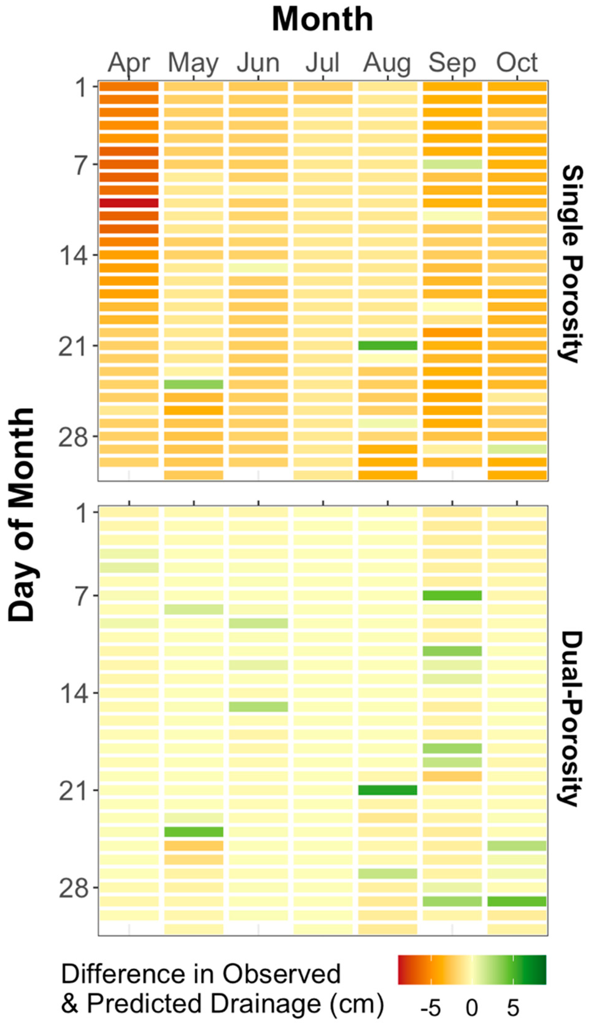
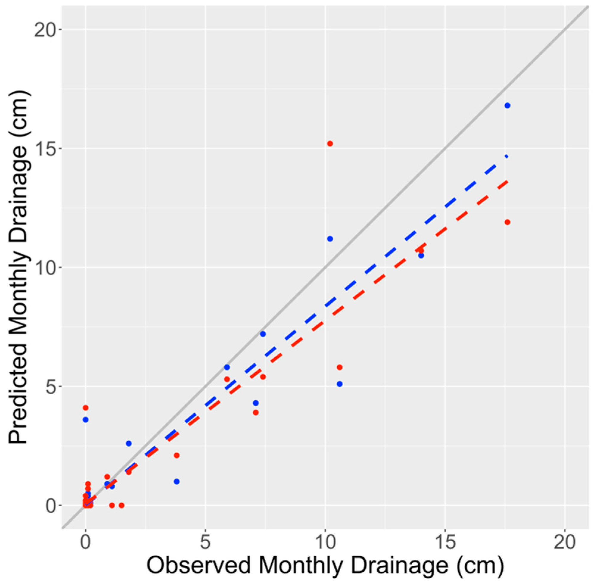
3.4. Simulated Model Runs

In the simulated model runs, differences in the monthly growing season drainage estimates between Hydrus-1D and WEPP depended on the facility, month, and treatment (two-, three-, and four-way interactions p-value < 0.001, Table S9). Much of this complexity derived from differences among the models, treatments, and facilities during April and May when drainage occurred, compared with little to no factor effects during June through to October. The four-way ANOVA test also showed a relatively small effect between the Hydrus-1D and WEPP models (F-value = 10, p-value = 0.002, Table S9) compared to other factors (F-value > 24, p-value < 0.001). The greatest monthly difference between Hydrus-1D and WEPP was 0.755 cm for the effluent-treated plots at Heyburn in April, but in August, this difference was only 0.076 cm (Figure 6 and Figure 7). Although Hydrus-1D and WEPP predicted significantly different monthly drainage values, both models agreed that drainage was predicted to occur in all growing season months except for May, June, and July. The predicted monthly drainage treatment response during the growing season depended on the facility and month for both Hydrus-1D (F*T × Mn p-value ≤ 0.001, Table S7) and WEPP (F × T × Mn, p-value ≤ 0.001, Table S8). These effects were caused by differences in the facility means between the control and effluent treatment groups in April and May.

4. Discussion

4.1. Observed Drainage

The increased drainage in the effluent-treated plots compared to the control plots during the growing season may have resulted from excess irrigation, elevated soil moisture, or altered soil properties. The facility irrigation logs indicated that the drainage that occurred during the end of the growing season (September and October) resulted from a combination of wastewater irrigation and precipitation. At one facility, (Garfield Bay) mechanical failure during the peak of summer forced application at the IWR in autumn (Figure 3), which was associated with September drainage. Excess irrigation was a likely cause of the increased drainage in the effluent-treated plots because it is an obvious hydrologic input that differed between the control and effluent plots at each facility. Irrigation schedules that minimize climatic factors such as precipitation and reduced transpiration with seasonal cooling may result in over-saturated soil. It is also possible that the increased drainage resulted from an altered soil water storage capacity, which can decrease with wastewater application potentially through the biological clogging of soil pores enhanced by nutrients in wastewater [41]. We observed increased microbiological activity in our effluent plots, supporting the suggested relationship by Cook et al. between reduced infiltration and increased microbiological activity [21]. Another likely factor causing this increased drainage was the elevated soil moisture content (Table 3), which accelerates the rate of soil water movement [19]. Potential drainage from irrigation can be further increased with the addition of water from a precipitation event, limiting the soil water storage capacity at the end of the growing season. Throughout the growing season, there was considerable variation in the collected drainage among facilities. In contrast to Garfield Bay, Ellisport Bay delayed irrigation while repairing storm damage and heavily irrigated during the late growing season in 2021, which did not result in drainage. This lack of observed drainage could have been due to low antecedent moisture content, high soil water storage capacity recharge, and the continued ability of trees to utilize soil moisture input in the late growing season.

The non-uniformity of irrigation within the plots may have affected the spatial drainage patterns at the FWR facilities. Vegetation blockage and irregular irrigation distribution could have resulted in variations in irrigation within the plots. This variation in irrigation due to the vegetation blockage of drain gauges and irregular irrigation distribution was illustrated between the effluent plots at all locations except Garfield Bay [27], which may have resulted in significantly different annual drainage measurements between the G3 and handmade drain gauges. As evidenced by some drain gauges, low-irrigation spots may drain a little, while high-irrigation spots may cause preferential flow [42]. Variation in soil moisture between wet and dry spots can magnify the variation in drainage. Areas receiving more irrigation are at a higher risk of initiating preferential flow and drainage.

The drainage observed with the drain gauges was seasonal, with little to no drainage occurring during the dry growing season and maximum flows occurring during the wet winter season (Table 4). During the peak months of drought (July and August), the drain gauges in the treatment plots did not receive any drainage as the soil remained relatively dry throughout the profile. Such a seasonal soil moisture pattern is commonly found in Pacific Northwest forests [43]. This agrees with the pattern observed with passive-wick drain gauges from a similar climate, where there was drainage during the wet season and little to no drainage during summer [23]. Drier soil and higher evapotranspiration rates during mid-summer may allow for an increase capacity to assimilate irrigation without the risk of drainage at these sites (Figure 3). Most of the observed drainage occurred during the dormant season months, when the soil water potential was high (Table 3). A high antecedent soil moisture resulting from snowmelt or precipitation increases the infiltration rate of the soil [20,44]. Antecedent soil moisture also influences deep soil drainage in forest systems [19]. A high soil moisture initiates preferential flow pathways through the soil profile as the soil moisture throughout the profile moves toward lower potentials [20]. The probability of preferential flow in large-diameter intact soil cores contained in drain gauge diversion tubes is expected to capture a higher drainage during the dormant season. Most precipitation that the facilities received during the dormant season fell as snow, as average hourly temperatures typically did not exceed 5 °C from November through to March (Table 3). Snow events and daily temperature fluctuations resulted in the rapid infiltration of snowmelt due to daily freeze–thaw fluctuations in the surface snow [44], which may also have caused a high observed drainage at these FWR facilities. An elevated antecedent soil moisture coupled with snowmelt flowing through preferential flow pathways may explain the high drainage occurring during the dormant season months. Quantification of this observed seasonal drainage pattern is crucial for the assessment of nutrient leaching across these FWR facilities, especially during the dormant season [21].

The drainage data that were observed with the drain gauges may have overestimated the drainage relative to that occurring outside of the diversion tube. This overestimation may have been due to the lack of tree roots and understory vegetation in the soil above the diversion tube that was removed during installation. This limits the direct effect of root water uptake and transpiration on the diversion tube connected to the drain gauge. Vegetation processes outside of the drain gauge included the root uptake of transpiration flow by the existing vegetation. More accurate measurements of drainage could be achieved through a combination of encouraging native vegetation root growth in the soil above the diversion tube and a postponement of drainage measurements to allow the site to heal after drain gauge installation.

Another cause of overestimation may have been due to the design of the diversion tube. Because the tube was made of an impervious material, water could not move horizontally between the tube and the soil surrounding it. This left mainly vertical water movement to occur within the tube, which may have resulted in the artificial development of macropores and preferential flow paths at the interface of the soil and diversion tube. The macropores would have increased the preferential flow in the diversion tube, increasing the amount of collected drainage in the reservoir and resulting in the overestimation of the collected drainage by the drain gauges.

4.2. Predicted Drainage and Assessment of Models

The drainage predictions confirmed that, regardless of the inherent differences in the purpose for each model, Hydrus-1D and WEPP have the potential to be used as support tools for FWR facility managers and regulators. In general, the models slightly underpredicted the growing season drainage compared to the collected drain gauge measurements (Figure 5). This consistent underprediction from the models may have been due to artificially high preferential flow paths caused by the diversion tube design, as discussed above, inaccurate soil hydraulic properties, or improper optimal precipitation and irrigation ratios provided to the models. While WEPP in particular had the capability to predict monthly drainage values throughout the year, it was less proficient during the dormant season, resulting in underpredictions of drainage. This lack of proficiency during the dormant season may have been due to an inability to accurately account for the daily freeze–thaw fluctuations in the surface precipitation that occurred at our project sites. WEPP may have been able to account for the daily freeze–thaw fluctuations in surface precipitation if the model was run on a daily or an hourly timestep.

The occasional overprediction of monthly drainage by Hydrus-1D during the growing season may have been related to its ability to model different soil, water, and vegetative physiological processes compared to WEPP. WEPP’s land management selection provides it with the capability to account for the effects of the temporal patterns of vegetation-related processes such as root water uptake and transpiration (e.g., [45]). Because Hydrus-1D does not have a land management selection, it lacks the acknowledgement of temporal shifts in plant growth throughout the model’s timescale. This was likely the cause of many of the differences in the drainage predictions and observations seen during the beginning and end of the growing season. WEPP required many climate-related input parameters, but had a simpler way to integrate these data into the model. As mentioned earlier, the soil input parameters were processed in different ways for each model, which may have been the source of some variations in the predicted drainage between models. Hydrus-1D had the capability to adjust many parameters involved with the soil hydraulic model, whereas WEPP did not have the ability to modify the soil hydraulic model at such a level. Another model that may be useful for facility managers and regulators to evaluate current plant available water conditions is an irrigation schedule model, such as Irrigation Scheduler Mobile [46]. Hydrus-1D and WEPP simulated similar monthly drainage values during the growing season, which supports the use of these models as adequate tools for wastewater irrigation decision making during the growing season.

Not without problems, we successfully parameterized Hydrus-1D and WEPP using drain gauge observations and soil input data to predict monthly drainage, similar to another study [47]. To improve the parameterization of both Hydrus-1D and WEPP, the estimated crop coefficient should be validated to provide the models with more accurate estimations of the daily evapotranspiration rate for the forests in this study. Previous studies have measured sap flux with evaporation and used those measurements to calibrate vegetation models [48,49]. This would provide quantitative measurements of the crop coefficients for these coniferous forests, as well as any seasonal and spatial variations in the crop coefficients. Alterations in the soil physical properties may also cause difficulties in parameterizing models in plots irrigated with wastewater. Previous studies have shown that soils irrigated with treated wastewater have altered soil properties [41,50]. The database used to gather information on the soil properties best represents control plot values, which may differ from the soil properties at study facilities subjected to prolonged wastewater irrigation. This highlights the need for site-specific measurements of soil hydraulic properties, such as hydraulic conductivity and residual and saturated water contents. In conjunction with site-specific soil hydraulic property measurements, the incorporation of advanced soil hydraulic models improves drainage prediction accuracy. As previously shown with irrigated soils, the dual-porosity hydraulic model of Hydrus-1D was capable of capturing the effect of macropore flow and produced agreeable results in the timing of drainage in this study (Figure 4 [51]). It would be beneficial for WEPP to incorporate preferential flow processes and fluid transport models into the soil hydraulic model. Regardless, the parameterized models were able to capture the magnitude and timing of drainage during the growing season (Figure 5). It is crucial for Hydrus-1D and WEPP to be able to account for the daily freeze–thaw fluctuations in the surface precipitation that occur in dormant season, and model drainage accurately during that time. A way to achieve this is by setting the models on an hourly timestep. This would require more model processing time, as well as hourly climate inputs, which may require hourly site-specific measurements of precipitation, irrigation, and evapotranspiration to improve the accuracy of the models.

5. Conclusions

Forests irrigated with wastewater experienced minimal drainage during the growing season, with an average of 0.96 cm of observed drainage per month. Most drainage during the growing season occurred in late spring and early fall, outside of the summer drought. Based on our drain gauge measurements, we suggest that irrigation should be primarily applied from June through to August, when substantially higher rates of wastewater can be applied with little environmental risk of leaching. However, seasonal adjustments to the crop coefficient may be required for the IWR targets throughout the spring and fall, while also accounting for the timing and duration of any precipitation events. During the dormant season, the monthly drainage from the effluent plots was as high as 46.1 cm. Large amounts of observed drainage occurring during the dormant season and the shoulder months of the growing season indicated a seasonal risk of constituent leaching. The high spatial variability of irrigation distribution suggested that localized leaching may occur throughout irrigation management units. Hydrologic models were able to successfully simulate drainage and could be useful support tools at FWR facilities to evaluate the leaching risk of this land application for various soil types and climates. Our results partially agreed with our hypotheses, in that (1) there was a significant treatment effect of wastewater irrigation at some facilities on drain-gauge measured drainage, and (2) the forests could assimilate permitted irrigation rates during the peak drought months of the growing season, but were incapable of doing so during the wet season. This study showed FWR as a viable option for communities to sustainably and efficiently reclaim wastewater, but it also highlighted that site and especially seasonally adaptive approaches for permitting are essential to minimize the adverse environmental risks associated with excess discharges to ground and surface water.

References

1. EPA. Guidelines for Water Reuse; EPA: Washington, DC, USA, 2012; pp. 1–643.
2. Wang, J.; Wang, G.; Wanyan, H. Treated wastewater irrigation effect on soil, crop and environment: Wastewater recycling in the loess area of China. J. Environ. Sci. 2007, 19, 1093–1099. [Google Scholar] [CrossRef]
3. Singh, P.; Deshbhratar, P.; Ramteke, D. Effects of sewage wastewater irrigation on soil properties, crop yield and environment. Agric. Water Manag. 2012, 103, 100–104. [Google Scholar] [CrossRef]
4. Kim, D.Y.; Burger, J.A. Nitrogen transformations and soil processes in a wastewater-irrigated, mature Appalachian hardwood forest. For. Ecol. Manag. 1997, 90, 1–11. [Google Scholar] [CrossRef]
5. Brister, G.; Schultz, R. The response of a southern Appalachian forest to waste water irrigation. J. Environ. Qual. 1981, 10, 148–153. [Google Scholar] [CrossRef]
6. Isebrands, J.G.; Richardson, J. Poplars and Willows: Trees for Society and the Environment; CABI: Rome Italy, 2014. [Google Scholar]
7. Gessel, S.; Miller, R.; Cole, D. Relative importance of water and nutrients on the growth of coast Douglas fir in the Pacific Northwest. For. Ecol. Manag. 1990, 30, 327–340. [Google Scholar] [CrossRef]
8. Hesse, I.; Day, J.; Doyle, T. Long-term growth enhancement of baldcypress (Taxodium distichum) from municipal wastewater application. Environ. Manag. 1998, 22, 119–127. [Google Scholar] [CrossRef]
9. Joshi, E.; Coleman, M.D. Tree Growth and Vegetation Diversity in Northern Idaho Forest Water Reclamation Facilities. Forests 2023, 14, 266. [Google Scholar] [CrossRef]
10. Jones, H.G. Irrigation scheduling: Advantages and pitfalls of plant-based methods. J. Exp. Bot. 2004, 55, 2427–2436. [Google Scholar] [CrossRef]
11. IDEQ. Guidance for Reclamation and Reuse of Municipal and Industrial Wastewater; IDEQ: Boise, ID, USA, 2007; pp. 1–563.
12. Docktor, D.; Palmer, P.L. Computation of the 1982 Kimberly-Penman and the Jensen-Haise Evapotranspiration Equations as Applied in the U.S. Bureau of Reclamation’s Pacific Northwest AgriMet Program; U.S. Bureau of Reclamation, Pacific Northwest Region, Water Conservation Center: Boise, ID, USA, 1994; pp. 1–28. [Google Scholar]
13. Pangle, R.; Kavanagh, K.; Duursma, R. Decline in canopy gas exchange with increasing tree height, atmospheric evaporative demand, and seasonal drought in co-occurring inland Pacific Northwest conifer species. Can. J. For. Res. 2015, 45, 1086–1101. [Google Scholar] [CrossRef]
14. Running, S.W.; Nemani, R.R.; Peterson, D.L.; Band, L.E.; Potts, D.F.; Pierce, L.L.; Spanner, M.A. Mapping regional forest evapotranspiration and photosynthesis by coupling satellite data with ecosystem simulation. Ecology 1989, 70, 1090–1101. [Google Scholar] [CrossRef]
15. Di Baccio, D.; Minnocci, A.; Sebastiani, L.; Carraro, V.; Grani, F.; Anfodillo, T.; Tognetti, R. Sap flow measurements for the evaluation of poplar clone performance in remediation of soil polluted with olive mill wastewater. In Proceedings of the VIII International Symposium on Sap Flow 951, Volterra, Italy, 8–12 May 2011; pp. 175–181. [Google Scholar]
16. Al-Jamal, M.; Sammis, T.; Mexal, J.; Picchioni, G.; Zachritz, W. A growth-irrigation scheduling model for wastewater use in forest production. Agric. Water Manag. 2002, 56, 57–79. [Google Scholar] [CrossRef]
17. Birch, A.L.; Emanuel, R.E.; James, A.L.; Nichols, E.G. Hydrologic impacts of municipal wastewater irrigation to a temperate forest watershed. J. Environ. Qual. 2016, 45, 1303–1312. [Google Scholar] [CrossRef] [PubMed]
18. Roygard, J.; Bolan, N.; Clothier, B.; Green, S.; Sims, R. Short rotation forestry for land treatment of effluent: A lysimeter study. Soil Res. 1999, 37, 983–992. [Google Scholar] [CrossRef]
19. Lai, X.; Liao, K.; Feng, H.; Zhu, Q. Responses of soil water percolation to dynamic interactions among rainfall, antecedent moisture and season in a forest site. J. Hydrol. 2016, 540, 565–573. [Google Scholar] [CrossRef]
20. Hardie, M.A.; Cotching, W.E.; Doyle, R.B.; Holz, G.; Lisson, S.; Mattern, K. Effect of antecedent soil moisture on preferential flow in a texture-contrast soil. J. Hydrol. 2011, 398, 191–201. [Google Scholar] [CrossRef]
21. Joshi, E.; Schwarzbach, M.R.; Briggs, B.; Coats, E.R.; Coleman, M.D. Nutrient Leaching Potential Along a Time Series of Forest Water Reclamation Facilities in Northern Idaho. J. Environ. Manag. in revision.
22. Gee, G.W.; Zhang, Z.; Ward, A.L.; Keller, J.M. Passive-wick water fluxmeters: Theory and practice. In Proceedings of the SuperSoil 2004: 3rd Australian New Zealand Soils Conference, Sydney, Australia, 5–9 December 2004. [Google Scholar]
23. Gee, G.W.; Newman, B.D.; Green, S.; Meissner, R.; Rupp, H.; Zhang, Z.; Keller, J.M.; Waugh, W.; Van der Velde, M.; Salazar, J. Passive wick fluxmeters: Design considerations and field applications. Water Resour. Res. 2009, 45, W04420. [Google Scholar] [CrossRef]
24. Zhu, Y.; Fox, R.; Toth, J. Leachate collection efficiency of zero-tension pan and passive capillary fiberglass wick lysimeters. Soil Sci. Soc. Am. J. 2002, 66, 37–43. [Google Scholar]
25. Meissner, R.; Rupp, H.; Seeger, J.; Ollesch, G.; Gee, G. A comparison of water flux measurements: Passive wick-samplers versus drainage lysimeters. Eur. J. Soil Sci. 2010, 61, 609–621. [Google Scholar] [CrossRef]
26. Hall, F. Protocol for Deployment and Operation of Deep Soil Percolation Sampler; Trim Number: 2018AGS1; Idaho Department of Environmental Quality: Idaho Falls, ID, USA, 2018; p. 43. [Google Scholar]
27. Clark, M.R. Measuring and Modeling Drainage in North Idaho Forest Water Reclamation Facilities; University of Idaho, ProQuest Dissertations Publishing: Moscow, ID, USA, 2022. [Google Scholar]
28. Schwarzbach, M.R. Forest Water Reclamation Project Dataset. 2023. [CrossRef]
29. USBR. AgriMet Weather Data. Available online: https://www.usbr.gov/pn/agrimet/h2ouse.html (accessed on 8 May 2024).
30. PRISM. Time Series Values for Individual Locations. Available online: https://www.prism.oregonstate.edu/explorer/ (accessed on 8 May 2024).
31. Lew, R.; Dobre, M.; Srivastava, A.; Brooks, E.S.; Elliot, W.J.; Robichaud, P.R.; Flanagan, D.C. WEPPcloud: An online watershed-scale hydrologic modeling tool. Part I. Model description. J. Hydrol. 2022, 608, 127603. [Google Scholar] [CrossRef]
32. NRCS. Web Soil Survey. Available online: https://websoilsurvey.sc.egov.usda.gov/App/WebSoilSurvey.aspx (accessed on 8 May 2024).
33. Clark, M.R. Predicting Soil Hydraulic Conductivity with RETC. Available online: https://youtu.be/PssFBRm5h5Q (accessed on 8 May 2024).
34. Schaap, M.G.; Leij, F.J.; Van Genuchten, M.T. Neural network analysis for hierarchical prediction of soil hydraulic properties. Soil Sci. Soc. Am. J. 1998, 62, 847–855. [Google Scholar] [CrossRef]
35. van Genuchten, M.T.; Leij, F.J.; Yates, S.R. The RETC Code for Quantifying the Hydraulic Functions of Unsaturated Soils; U.S. Environmental Protection Agency: Washington, DC, USA, 1991; 93p. [Google Scholar]
36. Molina, A.J.; del Campo, A.D. The effects of experimental thinning on throughfall and stemflow: A contribution towards hydrology-oriented silviculture in Aleppo pine plantations. For. Ecol. Manag. 2012, 269, 206–213. [Google Scholar] [CrossRef]
37. Fan, J.; Oestergaard, K.T.; Guyot, A.; Jensen, D.G.; Lockington, D.A. Spatial variability of throughfall and stemflow in an exotic pine plantation of subtropical coastal Australia. Hydrol. Process. 2015, 29, 793–804. [Google Scholar] [CrossRef]
38. Feddes, R.A. Simulation of Field Water Use and Crop Yield. In Simulation of Plant Growth and Crop Production; Pudoc: Wageningen, The Netherlands, 1982; pp. 194–209. [Google Scholar]
39. Jackson, R.B.; Canadell, J.; Ehleringer, J.R.; Mooney, H.; Sala, O.; Schulze, E.-D. A global analysis of root distributions for terrestrial biomes. Oecologia 1996, 108, 389–411. [Google Scholar] [CrossRef] [PubMed]
40. Moriasi, D.N.; Arnold, J.G.; Van Liew, M.W.; Bingner, R.L.; Harmel, R.D.; Veith, T.L. Model evaluation guidelines for systematic quantification of accuracy in watershed simulations. Trans. ASABE 2007, 50, 885–900. [Google Scholar] [CrossRef]
41. Cook, F.; Kelliher, F.; McMahon, S. Changes in infiltration and drainage during wastewater irrigation of a highly permeable soil. J. Environ. Qual. 1994, 23, 476–482. [Google Scholar] [CrossRef]
42. Nimmo, J.R. The processes of preferential flow in the unsaturated zone. Soil Sci. Soc. Am. J. 2021, 85, 1–27. [Google Scholar] [CrossRef]
43. Schmidt, A.; Mainwaring, D.B.; Maguire, D.A. Development of a tailored combination of machine learning approaches to model volumetric soil water content within a mesic forest in the Pacific Northwest. J. Hydrol. 2020, 588, 125044. [Google Scholar] [CrossRef]
44. Sutinen, R.; Hänninen, P.; Venäläinen, A. Effect of mild winter events on soil water content beneath snowpack. Cold Reg. Sci. Technol. 2008, 51, 56–67. [Google Scholar] [CrossRef]
45. Teskey, R.O.; Hinckley, T.M.; Grier, C.C. Temperature-induced change in the water relations of Abies amabilis (Dougl.) Forbes. Plant Physiol. 1984, 74, 77–80. [Google Scholar] [CrossRef] [PubMed]
46. Peters, T.; Hill, S. Irrigation Scheduler Mobile. Available online: http://irrigation.wsu.edu/Content/Resources/Irrigation-Scheduling-Aids-Tools.php (accessed on 8 May 2024).
47. Newcomer, M.E.; Gurdak, J.J.; Sklar, L.S.; Nanus, L. Urban recharge beneath low impact development and effects of climate variability and change. Water Resour. Res. 2014, 50, 1716–1734. [Google Scholar] [CrossRef]
48. Du, E.; Link, T.E.; Gravelle, J.A.; Hubbart, J.A. Validation and sensitivity test of the distributed hydrology soil-vegetation model (DHSVM) in a forested mountain watershed. Hydrol. Process. 2014, 28, 6196–6210. [Google Scholar] [CrossRef]
49. Wei, L.; Marshall, J.D.; Link, T.E.; Kavanagh, K.L.; Du, E.; Pangle, R.E.; Gag, P.J.; Ubierna, N. Constraining 3-PG with a new δ13 C submodel: A test using the δ13 C of tree rings. Plant Cell Environ. 2014, 37, 82–100. [Google Scholar] [CrossRef] [PubMed]
50. Leuther, F.; Schlüter, S.; Wallach, R.; Vogel, H.-J. Structure and hydraulic properties in soils under long-term irrigation with treated wastewater. Geoderma 2019, 333, 90–98. [Google Scholar] [CrossRef]
51. Wongkaew, A.; Saito, H.; Fujimaki, H.; Šimůnek, J. Numerical analysis of soil water dynamics in a soil column with an artificial capillary barrier growing leaf vegetables. Soil Use Manag. 2018, 34, 206–215. [Google Scholar] [CrossRef]
Figure 1. Map of the five wastewater facilities involved in study. They are located near Lake Pend Oreille and Lake Coeur d’Alene, which are shaded.
Hydrology 11 00087 g001
Figure 2. Diagram of a passive-wick drain gauge and its components. Two types of passive-wick drain gauges were installed: one was commercially built (G3 drain gauge, METER Group, Pullman, WA, USA) and one was “handmade” [26].
Hydrology 11 00087 g002
Figure 3. Total monthly rates of precipitation, irrigation water requirements (IWR), crop evapotranspiration (ET), and applied irrigation at each facility in 2021. Precipitation data gathered from PRISM, ET (alfalfa evapotranspiration rate × 0.7 crop coefficient) data gathered from AgriMet, and IWR and irrigation data gathered from IDEQ annual reports.
Hydrology 11 00087 g003
Figure 4. The total daily difference in observed and predicted drainage during the growing season for all drain gauge plots using Hydrus-1D. The top heatmap compared drainage predicted with the single-porosity van Genuchten–Mualem model to observed daily drainage, and the bottom heatmap compared drainage predicted with the Durner dual-porosity model to observed daily drainage. Root water uptake was excluded from these model predictions.
Hydrology 11 00087 g004
Figure 5. Observed and predicted values of monthly drainage during the growing season (April through October) at all drain gauge plots except for two effluent irrigated drain gauge plots at Cave Bay. Root water uptake was excluded from fine-tuned model predictions. Points are predicted drainage and dotted lines are best fit regression lines. Blue represents Hydrus-1D and red represents WEPP. Solid gray line is 1:1 line.
Hydrology 11 00087 g005
Figure 6. Predicted monthly drainage (cm) from Hydrus-1D-simulated runs averaged by facility. Error bars are standard errors. Mean separation letters indicate significant differences of predicted drainage between facilities within each month at α = 0.10. Root water uptake was included in simulated model predictions (Table S7).
Hydrology 11 00087 g006
Figure 7. Predicted monthly drainage (cm) from WEPP-simulated runs averaged by facility. Error bars are standard errors. Columns having the same letters are not significantly different among facilities within each month at α = 0.10. Root water uptake was included in simulated model predictions (Table S8).
Hydrology 11 00087 g007