Abstract
The municipal wellfield in Collierville, Tennessee, is contaminated with trichloroethylene (TCE) and hexavalent chromium (Cr (VI)) due to industrial operations dating back to the 1970s and 1980s. This study aims to elucidate the aquifer’s contaminant transport mechanisms by determining longitudinal and transverse dispersivities through inverse modeling. Utilizing MT3DMS for contaminant transport simulation, based on a well-calibrated groundwater flow model, and leveraging Python’s multiprocessing library for efficiency, the study employs a trial-and-error methodology. Key findings reveal that longitudinal dispersivity values range from 5.5 m near the source to 20.5 m further away, with horizontal and vertical transverse dispersivities between 0.28 m and 3.88 m and between 0.03 m and 0.08 m, respectively. These insights into the aquifer’s dispersivity coefficients, which reflect the scale-dependent nature of longitudinal dispersivity, are crucial for optimizing remediation strategies and achieving cleanup goals. This study underscores the importance of accurate parameter estimation in contaminant transport modeling and contributes to a better understanding of contaminant dynamics in the Collierville wellfield.
1. Introduction
Predicting the propagation of dissolved contaminants in an aquifer requires adequate characterization of transport parameters. Due to the unknown complexity of the subsurface system, these parameters are often assumed and rarely quantified at the required spatial resolution. Many transport models implement the advection–dispersion equation, which considers advection, mechanical dispersion, and diffusion along with other processes such as reaction and retardation. This dispersion parameter is crucial in describing the spreading of solute due to heterogeneity and is difficult to quantify due to its scale-dependent nature [1].
In many investigations, dispersivity is estimated through adjustments until the modeled concentrations best approximate observed concentrations [2,3,4,5,6,7,8,9,10,11,12]. An alternative approach to estimating dispersivity is through field and laboratory experiments conducted at different spatial scales [12,13,14,15,16,17,18,19,20,21,22]. However, field tracer tests are often time-consuming and very expensive. Some researchers attempted to upscale the laboratory-derived values to apply in field experiments [23], as well as to examine the scale-dependent nature [24] with comparison to field values [25]. However Refs. [26,27] showed that field-scale macrodispersion is intricately linked to subsurface heterogeneity, particularly affected by the integral scale and variance of log-conductivity and variance; thus, it cannot be assessed from the laboratory-scale experiment, which provides only a local dispersion.
Among the works conducted on dispersivities, ref. [28] conducted a critical review of 59 different field sites and found that longitudinal dispersivity ranged from 0.01 to 104 m for observational scales ranging from 0.1 to 105 m. Improving on that, [11] compiled 307 values of longitudinal dispersivity from 109 authors consisting of lab experiments, aquifer tests, and numerical models representing various types of aquifer media. They found that longitudinal dispersivity increases following a power law with the scale of measurement. Also highlighted in their study was a wide range of reported longitudinal dispersivity, 0.0003 to 30.5 m for an observation distance of 0.2 to 8800 m in unconsolidated sediments, and 0.0016 to 48.7 m at an observation distance of 0.035 and 3066 m in consolidated sediment [11]. These findings underscore the significant variability in longitudinal dispersivity across different scales and aquifer types, highlighting the complexity of accurately predicting solute transport in groundwater.
Numerical models offer a robust way to simulate contaminant transport on a larger scale in all three dimensions [3,4,29,30,31,32,33,34]. For a numerical model to simulate contaminant transport, a well-calibrated groundwater flow model is required to represent the flow field adequately. Given a properly defined boundary condition and starting concentration, a transport model can then predict the movement of a contaminant using the flow model results. Contaminants usually infiltrate groundwater systems via recharge mechanisms, subsequently dispersing through advection and dispersion processes. Calculating the hydrodynamic dispersion coefficient necessitates having data on the initial contaminant (or source) concentration and observed concentrations over time, derived from either an active contaminant plume or tracer studies. In numerical modeling, it is standard practice to apply a Dirichlet boundary condition (fixing concentration) at certain nodes of the grid, thereby generating a solute flux that results from both advective and dispersive movements [35]. Defining this initial source condition is crucial to avoid non-uniqueness against different dispersivity values, which is often very difficult to obtain in field studies.
In Shelby County, Tennessee, the primary drinking water aquifer is the semi-confined unconsolidated Memphis aquifer [36,37]. The aquifer is threatened by the presence of localized preferential pathways (i.e., breaches) in the overlying aquitard (the upper Claiborne confining unit—UCCU), warranting concern that contaminants could easily bypass the aquitard’s natural protection [38,39,40,41,42,43,44,45,46,47,48]. Very little is known about the contaminant transport properties of the Memphis aquifer. In Shelby County, Tennessee, one of the Town of Collierville’s five wellfields has been impacted by two contaminants: trichloroethylene (TCE) and hexavalent chromium (Cr(VI)). There exists limited source concentration data and few periodic measures of contaminant concentrations in downgradient monitoring wells. This site was chosen to ascertain estimated dispersivity values for the Memphis aquifer that may be used as initial values elsewhere in Shelby County owing to historical industrialization since the early 1900s and the potential contamination threat to other production wells (there are approximately 200 production wells in Shelby County). Scaled dispersivities are determined through a trial-and-error calibration approach between two plumes in the same area, something that is novel compared to other studies on scaled dispersivity where only a single contaminant plume was modeled. Results will show a relative increase in dispersivity with distance; however, there is some discrepancy in dispersivities over the same distance between plumes which is of interest. MODFLOW-NWT serves as the groundwater model and FloPy enables numerous MT3D simulations to arrive at scaled dispersivity values.
2. Materials and Methods
2.1. Study Area
In southeastern Shelby County, Tennessee, the Town of Collierville was selected because of the impact on one of Collierville’s five wellfields by two U.S. Environmental Protection Agency (EPA) Superfund sites, which include TCE and Cr (VI) as contaminants of concern (Figure 1). As shown in Figure 1, Collierville’s Wellfield #2 (WF2) is positioned north-northwest and downgradient from the Carrier facility and is 0.8 km to the west and also downgradient from Smalley Piper. WF2 came online in 1967, producing 6166 m3/d of water for domestic consumption from two wells that are screened in the Memphis aquifer at depths of 87.5 m (COLL-201) and 98.7 m (COLL-202).
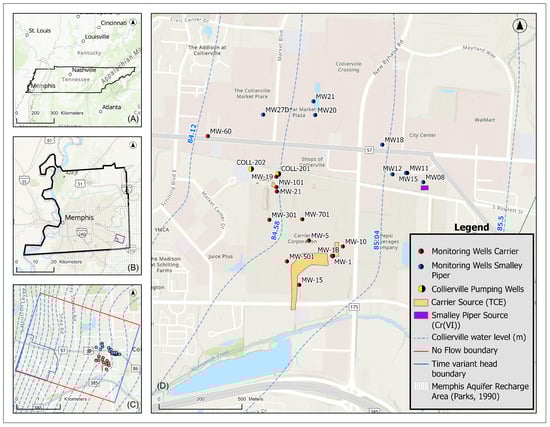
Figure 1.
All monitoring well locations for Carrier and Smalley Piper: (A) State of Tennessee, (B) CAESER II model boundary, (C) Submodel Boundary, (D) Study Area.
Shelby County sits within nearly square in the middle of the the northern Mississippi embayment, a basin filled with over a thousand meters of unconsolidated sediments from the Cretaceous to Quaternary periods, as detailed by [27,49]. This results in a complex geological structure featuring gently dipping early to mid-Tertiary geologic units of unconsolidated sand, silt, clay, and minor lignite, as described in the Coastal Plain setting, with Pleistocene and Pliocene fluvial-terrace deposits of sand and gravel, 0 to 20 m thick, atop them [50]. Loess deposits, 3 to 20 m thick, excluding the valleys filled with up to 15 m of late Pleistocene to Holocene alluvium, cover the landscape, as shown by [51].
Hydrostratigraphically, the area is divided into several units: the loess and upper alluvium act as a leaky, weak confining layer, with similar textural and hydraulic properties [51], while the fluvial-terrace and lower alluvium deposits form the Shallow aquifer [27]. Below this, the Cockfield and Cook Mountain formations create the upper Claiborne confining unit to the sand-dominated Memphis aquifer, which has a significant transmissivity (average 3.25 × 10³ m2/day) or hydraulic conductivity (average 14.9 m/day) [38,51,52,53]. The Flour Island Formation then serves as the lower confining unit to the Memphis aquifer and the upper confining unit to the Fort Pillow aquifer, further highlighting the region’s intricate hydrogeological structure.
The Upper Claiborne Confining clay (UCCU), upper aquitard to the Memphis aquifer, exists under much of Shelby County except to the east where there are subcrops and the Memphis aquifer transitions from confined to unconfined—this transition occurs beneath Collierville [27,54], thereby making it easier for anthropogenic contaminants to reach the aquifer [27,38].
2.1.1. Carrier Corporation
The Carrier site began operations in 1967, producing air conditioning units. In 1979, a vapor degreaser unit failed, leaking approximately 7500 to 19,000 L of TCE on the southeast side of the property (Figure 1). Carrier also had an unlined 6 m3 lagoon operational since 1972 (Figure 1) for storing TCE-contaminated paint sludge. This lagoon was filled in 1980. After a heavy rainfall in 1985, Carrier discovered that an unknown quantity of TCE leaked from underground pipes associated with an above-ground TCE storage tank (Figure 1), all of which was removed within a month after the spill. Approximately 2052 L of TCE were recovered. The following year, in 1986, low levels of TCE were detected in the nearby wellfield (WF2), subsequently listed as a U.S. EPA Superfund site in 1990. WF2 continued to operate until December 2003, until hexavalent chromium from the nearby Smalley Piper was detected in the WF2 production wells.
Forty-three monitoring wells were installed between 1986 and 2016 for monitoring and remediation purposes at the site. An expansion of the main building in 2004 closed many wells whose historical locations could not determined. Among the remaining wells, 19 wells were determined to have either concentration data, groundwater level data, or both at various times. The locations of all the wells are shown in (Figure 1). Among those 19 wells, 12 were selected to use in this study. Monitoring wells MW-3, MW-4, and MW-601 are hydrologically upgradient wells (Figure 1). Based on historical concentration measurements onsite, MW-3 had a concentration one order of magnitude higher than MW-4 in the period of 1987–1989; however, these two wells are spatially 2.34 m apart, are separated 9 m vertically, and are screened within the same hydrogeologic unit. Subsequently, no reason can be offered as to their drastic differences in concentration, thereby making them not suitable to use in the numerical model as they fall in the same grid cell where an average concentration is calculated. Six wells among the twelve, namely, MW-1, MW-1B, MW-10, MW-15, MW-19, and MW-21, were used to determine the source concentration of the three sources (1979 spill, 1985 spill, and unlined lagoon). The remaining six wells (MW-5, MW-101, MW-301, MW-501, MW-701, and MW-60) were used to find dispersivity values and are shown in (Figure 1).
2.1.2. Smalley Piper
The second Superfund site, Smalley Piper, manufactured magnesium battery casings from 1970 to 1981. This site had two tarpaulin-lined ponds for treating chromic acid-induced wastewater [55] (Figure 1). Approximately 2 m3 of chromic acid were discharged once a week via an underground pipe into the treatment ponds, where liquid sulfur dioxide (SO2) was injected twice per week to precipitate chromic sulfide as less toxic trivalent chromium. However, the reaction efficiency depended on the quantity of SO2 and mixing, and incomplete reactions resulted in hexavalent chromium present in the wastewater [55].
The remaining wastewater (100 m3/day) containing hexavalent chromium was discharged into onsite drainage ditches that flowed into Nonconnah Creek, approximately 0.4 km south of the facility. The manufacturing operation ceased in 1981–1982, and the treatment ponds were closed. Since 2007, the former industrial processing buildings on the western portion of the site remained, while the eastern portion of the site had been redeveloped and is currently operating as a public mini-storage facility [56].
A groundwater remediation investigation conducted in 2004 determined that the highest concentrations of Cr(VI) were found 23 to 30.5 m below land surface (bls), with concentrations ranging from 20,000 to more than 250,000 micrograms per liter (µg/L). Groundwater samples from depths greater than 30.5 m bls exhibited total chromium concentrations below the 100 µg/L maximum contaminant level (MCL) specified by the World Health Organization and U.S. EPA [57]. Chromium contamination was not detected in groundwater collected from the eastern part of the property boundary, which is hydrologically upgradient of the site (Figure 1). A total of 21 monitoring wells were installed between 2002 and 2006. Among those twenty-one wells, eight wells (Figure 1) were selected for this study due to the quality of data. Among these eight wells, MW-8 was used to define the source concentration and the remaining seven wells (MW-11, MW-15, MW-12, MW-18, MW-20, MW-21, and MW-27D) were used to determine dispersivity values.
2.1.3. Numerical Flow Model
The Collierville area was included in a prior, calibrated groundwater model (i.e., CAESER II) that simulated groundwater conditions beneath Shelby County between 1960 and 2021 within the shallow Memphis and Fort Pillow aquifers [58]. CAESER-II is an updated model based on [59] (i.e., CAESER-I), which simulates the multi-layer aquifer system in the Shelby County area with a cell size of 250 m by 250 m using MODFLOW-NWT. In CAESER-II, the shallow aquifer was represented as one layer, the UCCU as one layer, the Memphis aquifer as four layers, the Flour Island confining unit as one layer, and the Fort Pillow aquifer as one layer. The authors of [58] extended CAESER-I from 2005 back to 1960 to account for flow conditions during the time when most contaminant spills in the area occurred, recalibrating the model with updated Memphis aquifer properties based on [60], historical pumping data, and hydraulic conductivities measured on a borehole sample obtained from a UCCU breach [58]. All adjusted parameters and calibration metrics for CAESER-II can be found in [58].
A submodel was created from CAESER-II to conduct contaminant transport modeling. The Town of Collierville is isolated from other pumping from the Memphis aquifer and the projection of contaminant migration does not extend far within the model (e.g., westward to the City of Germantown, which has its own production wells); hence, using a submodel was appropriate. Additionally, preliminary testing of contaminant transport using CAESER-II indicated extraordinary long run times due to the size of the model; therefore, using a submodel would reduce runtime without necessitating areas simulated by CAESER-II not relevant to the Collierville area.
The submodel’s extents greatly exceeded anticipated distances that contamination may travel to avoid boundary effects. Following the regional groundwater gradient of the Memphis aquifer, the submodel paralleled the orientation of CAESER-II to a southeast to northwest direction II (see Figure 1, insets B and C). Using the same stress periods as CAESER-II, the resulting heads from CAESER-II defined the eastern and western boundary conditions as time-variant heads. Due to the submodel’s orientation to align with the Memphis aquifer gradient [61], the northern and southern boundaries were set as no-flow. The submodel has 736 stress periods spanning from 1960 to 2021. Unlike CAESER-II having square cells of 250 m, submodel cell sizes were reduced to 50 m square, resulting in 79 rows by 101 columns. The vertical representation increased from 8 to 24 layers (Figure 2). These modifications to cell dimensions and number of layers were made to accommodate various contaminant source locations (i.e., isolating them to a single cell or the flexibility to be active across multiple cells) and to obtain a more discretized movement of contamination vertically within the system based on monitoring well observations. The shallow aquifer was represented by two layers, the UCCU remained as one layer, the Memphis aquifer went from four layers to fourteen, the Flour Island confining unit was four layers, and the Fort Pillow aquifer was also four layers (Table 1).
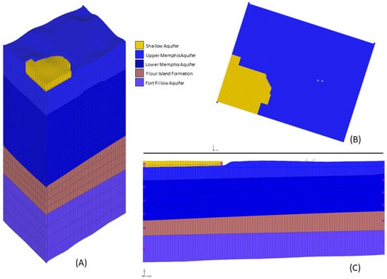
Figure 2.
Plan view of the model extent and model grid with different hydrogeological units. (A) The 3D Grid, (B) Plan View, and (C) Cross-section of model (10× vertical exaggeration).

Table 1.
Average layer thicknesses in submodel.
As would be expected, changing cell dimensions (spatially and vertically) from a parent model with larger cell sizes (i.e., 5 time larger) requires redistribution of aquifer characteristics. As CAESER-II represents a calibrated model using PEST, resultant values of hydraulic conductivity (K), specific storage (Ss), and specific yield (Sy) varied from cell to cell. To define these parameters to the submodel cell configuration, values were interpolated using inverse distance weighting (IDW) from CAESER-II onto the finer grid of the submodel (Table 2).
Table 2.
Parameters range for submodel simulation.
A time-dependent specified head boundary condition was implemented for the shallow aquifer. For the Memphis aquifer, a time-variant head was implemented in the eastern and western boundaries, while the north and south boundaries were kept no-flow based on historical water level maps [61]. The Flour Island and Fort Pillow boundaries were mimicked as as no-flow at the submodel scale following that of the parent model [58,59]. To determine the accuracy of submodel conditions to that of the parent model (CAESER-II), two analyses were performed: a zonal flow budget comparison of the submodel to the same area represented in CAESER-II and an error analysis of heads on a cell-by-cell basis. As can be seen from Table 3, budget values between the two models shifted between 0 and 0.16 m3/day.
Table 3.
Flow budget comparison between CAESER-II and the submodel.
Submodel heads were simulated from 1960 to 2021 using MODFLOW-NWT [62]. A cell-by-cell head comparison between the submodel and CAESER-II was performed and, submodel heads were within 0.17 m of CAESER-II; therefore, recalibration was deemed unnecessary.
2.1.4. Contaminant Transport Model
The contaminant transport model was developed using MT3DMS. Assuming conservative conditions, as there was no data to suggest otherwise, the contaminant transport model was calibrated and verified against the observed concentrations in the monitoring wells. Adjusted input parameters were longitudinal and transverse (horizontal and vertical) dispersivities. The source boundary conditions and initial concentration values were defined based on historical contaminant data from the monitoring wells adjacent to the source.
Source concentration plays a vital role in concentration distribution, and a time-variant specified concentration boundary (Dirichlet) was defined for both sites. These boundaries are termed “source function” and mimic the increase, saturation, and decrease in concentration in groundwater through a rising limb, a plateau, and a receding limb, respectively (Figure 3). The length of each limb was determined from field data adjacent to the source. Monitoring well MW-15 was used to define the source function for the 1979 spill, MW-19 and MW-21 were used for the unlined lagoon, and MW-1, MW-1B, and MW-10 were used for the 1985 spill at the Carrier site. For the Smalley Piper site, data from MW-8 were used.
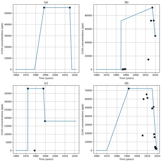
Figure 3.
Contaminant source functions for (a) 1979 Carrier Spill, (b) 1985 Carrier Spill, (c) Unlined lagoon, and (d) 1970 Smalley Piper Source. Black Squares represent measured concentrations.
Regarding spatial distribution of the sources, the unlined lagoon, Smalley Piper, and the 1985 Carrier spills each were represented by a single model cell. Conversely, the source for the 1979 TCE spill at the Carrier site spanned across three model cells. All sources were applied in layer 3 of the Memphis aquifer, which represented the first layer of entry either below its upper confining unit (i.e., UCCU) or from the shallow aquifer where the Memphis aquifer was locally unconfined.
Of note, Ref. [63] infers the existence of the UCCU (termed Jackson Clay in report) near the vicinity of the Carrier plant. Ref. [38] shows the Carrier facility and all monitoring wells within the Memphis aquifer unconfined zone, absent of the UCCU; however, ref. [64] indicates the opposite being most confined. With greater detail of the subsurface provided by [63], contaminant sources at Carrier fell either on the fringe of the UCCU subcrop (by 1–2 cell sizes) or outside its influence. Hence, it was assumed that dissolved phase TCE entered the Memphis aquifer and was not impacted by the UCCU.
Advection in MT3DMS was solved using a third-order TVD (total-variation-diminishing) scheme which is mass conservative and minimizes numerical dispersion and artificial oscillation. It is understood that porosity does change slightly, simply owing to the range of hydraulic conductivities shown in Table 2. It was also realized that the option of cell-by-cell alteration of porosity was constrained by the lack of comprehensive field data required for such detailed adjustments. Therefore, following the works by [64,65], who defined porosity locally in the area, a sensitivity analysis on porosity was not deemed necessary and a value of 0.3 was applied. For each iteration in defining dispersivities, a combination of longitudinal, transverse horizontal, and transverse vertical dispersivity values were assigned across the model domain and RMSE (root mean squared error) values at each monitoring well were calculated against observed concentrations.
To gauge initial values of dispersivity for use in the model, a range of possible values were applied until a reduction in RMSE was realized. Once a range was obtained (see Table 4), a straightforward trial-and-error method was implemented for calibration instead of using optimization tools like PEST or UCODE because there are not enough supporting studies that use these tools for this type of calibration. Additionally, the approximated source concentrations were based on nearby monitoring well concentrations. As will be shown, there is much scatter in the observed readings of contaminant concentrations; hence, an analysis based on point value comparisons was not conducted. Instead, an overall concentration trend match was attained. This type of calibration has been successfully demonstrated by [4,34,66,67]. Of note, no dry cells were observed in the MODFLOW-NWT solutions, which eliminated the possibility of contaminant mass accumulation in cells.
Table 4.
Dispersivity values for MT3DMS simulation.
The inverse transport simulations were performed using the FloPy Python package (v3.3.4) [68] and MT3DMS (v5.3) [69]. The FloPy script executed the MT3DMS transport model for both TCE and Cr(VI) plumes for different combinations of dispersivity values following a workflow like [11]. The scripted workflow is illustrated in Figure 4. An iterative process was conducted by implementing enumerable combinations of longitudinal, transverse horizontal, and transverse vertical dispersivities within the ranges shown in Table 4 and incremented using the step jumps of 0.5, 0.01, and 0.001, respectively, for each match to a monitoring well, resulting in tens of thousands of independent model runs. Hence, a suite of dispersivity combinations would be applied globally to the model and a comparison made between the modeled concentration and observed concentration for each well, then the same process would be performed for each monitoring well thereafter to provide a better estimation (and realization) of scale-dependent dispersivity.
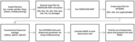
Figure 4.
Inverse MT3DMS workflow.
To improve the computational efficiency of conducting numerous MT3DMS model runs, the Python multiprocessing library was used. The runtime was significantly reduced from 30 h to 3.5 h using an 8-core Intel Core i7-9700 CPU.
3. Results
3.1. Simulated vs. Observed Concentration
Simulated and observed concentration plots for the Carrier and Smalley Piper sites are shown in Figure 5 and Figure 6, respectively. The resulting dispersivity values for each well for both sites are given in Table 5 (Carrier) and Table 6 (Smalley Piper).
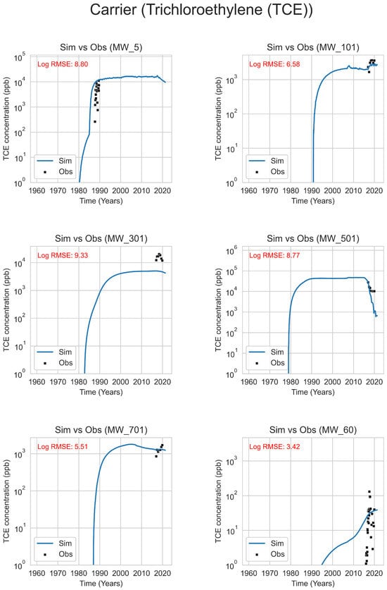
Figure 5.
Carrier simulation vs. Observation data (MW-5, MW-101, MW-301, MW-501, MW-701, and MW-60). Concentrations are in log scale with well locations shown in Figure 1.
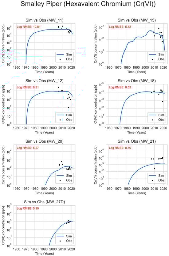
Figure 6.
Smalley Piper simulation vs. Observation data (MW-11, MW-15, MW-12, MW-18, MW-20, MW-21, and MW-27D). Concentrations are in log scale with well locations shown in Figure 1.
Table 5.
Dispersivity Values (Carrier Site).
Table 6.
Dispersivity values (Smalley Piper site).
Figure 5 shows the simulated vs. observed concentration of TCE in six monitoring wells. Among them, MW-5 is one of the earliest wells installed onsite with data available from 1987 to 1988. The other wells have concentration data from 2010 to 2019. From the analysis, longitudinal dispersivity values at the Carrier site range from 10.5 to 55.5 m, transverse horizontal values range from 1.27 to 24.97 m, and vertical dispersivity from 0.42 to 2.22 m (Table 5). The distance between the source and monitoring well is given as L(m) in Table 5. The closest well, MW-5, had the lowest longitudinal dispersivity among all wells; however, its transverse horizontal dispersivity at first seems high yet is impacted by two sources making deciphering values to distance more challenging. MW-101 is only 31 m from the lagoon source in 1979, which would imply a lower longitudinal dispersivity than MW-5, whose shortest distance is nearly 183 m from the 1985 source. However, samples in MW-101 were not taken until 2010, well after any of the three sources started leaking. MW-501 is closer to sources than MW-101 and MW-301, resulting in lower dispersivity values. MW-701 was slightly further away from sources than MW-501 but with less distance than MW-101 and MW-301, resulting in dispersivities higher and lower, respectively. Interesting is MW-60, which is further from the 1979 and 1985 sources than all other wells, yet has the second lowest longitudinal dispersivity among the wells; however, this well is also only 448.28 m from the 1979 lagoon source. MW-60 had the largest concentration spread than the other wells, ranging over two orders of magnitude; however, it had the lowest log RMSE at 3.42.
Figure 6 shows the simulated vs. observed hexavalent chromium concentration at the Smalley Piper site. All seven observation wells have data ranging from 2005 to 2019. From the analysis, longitudinal dispersivity values at this site range from 5.5 m to 55.5 m, transverse horizontal values range from 0.28 m to 24.98 m, and transverse vertical dispersivity from 0.03 m to 2.5 m (Table 6). The two closest wells, MW-11 and MW-15, each just under 90 m from the source, indicated low longitudinal dispersivity, as would be expected for a scale-dependent parameter. Interestingly, MW-12 at 156.15 m from the source had a higher longitudinal dispersivity (more than twice) and transverse dispersivity (just less than three times) than the next furthest well, MW-18, at nearly 220 m from the source; however, it matched these same values for MW-21 at 750.91 m from the source, or almost five times the distance. The furthest well, MW-27D, had dispersivity values lower than the third furthest well, MW-12.
3.2. Comparison with Empirical Dispersivity Equations
Dispersivity values obtained for both sites were compared against three empirical equations shown in Table 7. Among the equations used, Gelhar and Schulze-Makuch imply a direct proportional relation between observed distance and longitudinal dispersivity where Schulze-Makuch’s implies a slower increase of longitudinal dispersivity with distance. Xu and Eckstein’s equation also implies slowing down at a larger scale and captures non-linear behavior natural aquifers. Both Schulze-Makuch and Xu–Eckstein’s equation suggests a plateau at larger distances where the sensitivity to scale of longitudinal dispersivity diminishes.
Table 7.
Empirical equations of longitudinal dispersivity.
Table 8 and Table 9 show the calculated and optimized values of longitudinal dispersivity for the Carrier and Smalley Piper sites.
Table 8.
Comparison of longitudinal dispersivity values (m) with empirical equations and effective lengths (Carrier site).
Table 9.
Comparison of longitudinal dispersivity values (m) with empirical equations (Smalley Piper site).
The effective length, , was calculated as a weighted average of peak concentrations of the three sources, using the following formula:
where the weights (w) are proportional to the concentrations of contaminants measured in those years, such that:
and .
From the analyses presented in Table 8 and Table 9, it is evident that there is not a consensus that one empirical model better matches modeled longitudinal dispersivities to the other equations. At the shorter distances, such as for MW-5, MW-11, and MW-15, values are reasonable comparable across the three empirical equations. At greater distances, Gelhar (1992) [28] overestimates hydraulic conductivity where Xu and Eckstein (1995) [70] and Schulze-Makuch (2005) [11] are within reason (see MW-60 in Table 8 and MW-27D in Table 9).
4. Discussion
The primary goal of this study was to derive the range of longitudinal, transverse horizontal, and transverse vertical dispersivities by matching observed contaminant data against modeled concentrations and to assess the presence of longitudinal dispersivity scale dependency. Additionally, FloPy was employed in a novel way to concurrently run parameterized MT3DMS simulations, reducing the overall simulation runtime by a factor of eight. What is interesting about this investigation compared to others in the literature is the presence of two distinct plumes from two separate industries, Carrier and Smalley Piper, which for similar distances between source and monitoring well indicated notably different dispersivities.
As with many investigations into contaminant transport, obtaining the original source concentration proves difficult. This investigation is no exception, whereby no original source concentrations were available and concentrations at the closest monitoring wells were used to derive source concentrations. For the Carrier 1979 spill, only two readings existed near the source, spanning nearly 30 years between the readings. The Carrier 1979 unlined lagoon source function was complicated as concentrations from MW-19 and MW-21 offered a wide spread in concentrations, varying from 0 to over 35,000 mg/L bracketing the lagoon discharge of 1979 by plus-minus a decade. The 1985 Carrier spill had three nearby monitoring wells with multiple concentration readings enabled, except for a single, low reading in 2012. The Smalley Piper was a newer incident and therefore had more available data, though scattered to a degree.
The Carrier site was also complicated by having three sources separated by six years and of varying size, with the 1979 spill covering the largest area on the southern portion of the property. Carrier wells, namely, MW-5, MW-101, MW-501, and MW-701 demonstrated a relatively good agreement between observed and model simulation concentrations whereby the simulated concentration trend fell within the cluster of concentration readings, with the slight exception of MW-5 (log RMSE of 8.80) due to a predicted early arrival. The log RMSE values corroborate this assessment with MW-101, MW-501, and MW-701 having lower log RMSE values than the under-matched trends on MW-301 and MW-601.
Surprisingly, MW-60 had the lowest log RMSE (3.42) though the largest scatter with observed concentrations bracketing the modeled trend above and below. The undershot of the model concentration trend to the observed concentrations in wells MW-301 and MW-601 (Figure 5) could be improved by a higher advective component, which would bring into question the accuracy of the simulated heads for the Memphis aquifer. In CAESER-I, Ref. [59] used PEST to calibrate the model. Unfortunately, no control points existed in the Collierville area. Likewise, Ref. [58] for CAESER-II used the same control points as [59] but extended some control further back in time to 1960 where data existed. Hence, the heads in CAESER-II and subsequently the submodel received questionable calibration. There does exist some historical water level data in [71] that contrast the resulting submodel generated heads (Table 10), with the prior being consistently higher.
Table 10.
Water level data.
Among the historical water level data, MW-1, MW-1A, and MW-1B are within 3.5 m of each other and are of similar depth, but they exhibit a head difference of only 3 m, thereby raising questions into these readings. MW-5 indicated a water level of 94.28 m above mean sea level (amsl) in 1988, where under predevelopment conditions (1886), the groundwater level in downtown Collierville (about 2.3 km upgradient) was estimated to be 90 m amsl [72]. Furthermore, ref. [61] estimated the water level in the Collierville area to be 85.34 m which is a mere 4.66 m change in 101 years.
Submodel data show a water level difference of 2 to 5 m compared to the historical data in most wells, except for MW-5. More recently, a groundwater assessment performed for the Town of Collierville by the Center for Applied Earth Science and Engineering Research (CAESER) in 2018/2019 showed groundwater levels to be between 84 and 85 m, which is consistent with the submodel generated head values [73]. Ignoring the historical data obtained from the reports (i.e., [71]) due to questionable measurement disparities and relying more on these other measures [61,72], there is no reason to assume a possible shift in submodel gradients and, hence, change in advection.
The various values of dispersivities by well (Table 5 and Table 6) illustrate scale-dependency of this parameter, where consistently between Carrier and Smalley Piper the shortest distance wells (MW-5, MW-ll, and MW-15) have much lower longitudinal dispersivities than for those well further away. However, the premise of scale-dependency of an increasing value with distance is a challenge to observe from our results. Taking the furthest two wells (MW-60 and MW-27D), the calculated longitudinal dispersivities were less than the second furthest wells in each dataset, MW-501 at 119.90 m (ignoring MW-101) and MW-12 at 156.15 m, respectively. With the highest longitudinal dispersivity at each site at 55.5 m, it would stand to reason that MW-60 and MW-27D, with longitudinal dispersivities of 20.5 and 15.5, respectively, would be higher than 55.5 m.
MW-60 at Carrier is over 900 m from the two spills on the south end of the plant, but is 448.28 m from the lagoon source (1979). MW-301, being approximately 380 m and 430 m from the two southern sources, hence, near the same distance as MW-60 from the lagoon, had a longitudinal dispersivity of more than twice MW-60 at 55.5 m. Being that the 1979 lagoon source had a concentration half that of the other spills and spanned fewer decades than the larger spills, adds to the complexity of MW-60, as can it be observed very large scatter of concentration readings between 2016 and 2019 (see Figure 5 for MW-60). Hence, obtaining a good longitudinal dispersivity proved challenging.
Though not incorporated at the time of modeling due to missing screen depth information, two observation wells, MW1101 and MW1201, located 360 m and 440 m, respectively, southwest of MW19 (near COLL201 and COLL202, the Collierville Wellfield #2, see Figure 1), indicated near non-detect (ND) TCE concentrations between March 2018 and November 2019. This would suggest that pumping from Wellfield #2 was capturing the TCE plume. However, ignoring dispersion and relying solely on groundwater gradients and wellfield pumping as simulated in the calibrated numerical model, TCE concentrations are not captured by the wellfield and instead there are elevated concentrations of TCE at MW1101 and MW1201. We do not dispute the observed concentrations yet have observed wide variations in measured TCE concentrations, for example, see Figure 3c. Such fluctuations in observed readings are not uncommon, as [74] observed in TCE concentrations where they dropped four orders of magnitude in a 3-month period to near ND only to rise back to prior concentrations a few months later. In such cases, TCE concentration trends were used to define plumes; hence, we cannot always match acute TCE concentrations such as those observed in MW1101 and MW1201.
The Smalley Piper well, MW-27D, at 954.42 m from the source had the second lowest log RMSE with the lowest being MW-27, although MW-27 had much more scatter in its readings over a period of nearly 12 years than MW-27D with readings over a smaller time period (5 years). However, Xu and Eckstein’s (1995) and Schulze-Makuch’s (2005) empirical equations suggest near similar longitudinal dispersivities to MW-27D (15.5 m) at 11.58 m and 22.03 m, respectively. This does not necessarily discount Gelhar’s empirical equation, which produced at longitudinal dispersivity of approximately 95 m where the maximum [28] found from their review was 104 m. Certainly, all three empirical equations adhere to the scale-dependency concept of increasing dispersivity with distance, making a direct comparison difficult with the results of this study.
At Carrier, aside from MW-60, the other monitoring wells do adhere more closely to an increased dispersivity with increasing distance, although having three spatially and temporally different sources add a lot of complexity to this site. Interestingly, MW-101 and MW-301 share the same dispersivity values. This is because these wells are reaching the threshold constraints as stated in Table 4. MW-101 seems to match the observed data well (see Figure 5) and has the third lowest log RMSE at 6.58. The readings are clustered tightly like MW-301; however, the concentration trend fails to pass through its cluster of readings.
If the thresholds in Table 4 were to be expanded, which fall between [11,28], then the transverse horizontal and transverse vertical could be reduced to move more mass longitudinally and possible have the concentration trend pass through the MW-3-1 cluster. However, doing so would result in a counter-intuitive longitudinal dispersivity as it would be larger than MW-101 even though MW-101 is further away from MW-301 by 70–160 m from the southern sources. Then again, the fact that MW-101 is a mere 31 m from the lagoon source adds reason for a possible lower longitudinal dispersivity than MW-301, yet why is it not much lower like MW-5, which is further from its sources (between 182.75 and 232.94 m) and has the lowest longitudinal dispersivity (10.5 m)?
Lastly, MW-501 had a longitudinal dispersivity of 25.5 m even though it is only 119.9 m from the 1979 source, which, based on scale dependency, would imply a lower longitudinal dispersivity. This may be attributed to high variability of concentrations at MW-15, which was used to define the 1979 source. In the period of record (1987–1989), MW-15 had concentrations varying two orders of magnitude with a peak value of 400,000 ppb in June 1989, yet two months prior (April) had a measured concentration of 140,000 ppb and 5900 ppb in January of that same year. This dramatic fluctuation in concentrations leads to misinterpretation of source history (likely overestimation), therefore manifesting a high dispersivity to match declining concentrations in observation well MW-501.
Smalley Piper’s monitoring wells produced similar dispersivity oddities to those seen with Carrier. MW-12 and MW-21 both pressed against the imposed thresholds like with MW-101 and MW-301 at Carrier. Both MW-12 and MW-21 had scattered readings across nearly three orders of magnitude to about two orders of magnitude, respectively, and both had the highest log RMSE errors at 8.91 and 8.70, respectively. Strangely, MW-12 is extremely close to the source at 156.15 m and MW-21 is almost five times further away. Hence, it is difficult to say that one or both of these wells’ dispersivities can be trusted. To the contrary, MW-20 and MW-27D are both distant from the source at approximately 695 m and 954 m, respectively, and with the same dispersivities. The concentration trend for MW-27D passes through its cluster of readings (see Figure 6); however, for MW-20 there is a bit more scatter and the concentration trend it is forced to pass between are two clusters around 2007–2010 and 2014–2018. Yet again, we see a mid-distance well, MW-18, at 219.19 m from the source with a higher longitudinal dispersivity than the farther wells, MW-20 and MW-27D, yet lower than MW-12 (longitudinal dispersivity of 55.5 m), which is closer to the source at 156.15 m.
Part of this discrepancy is complicated by the observed concentration readings as some seem either difficult to believe or it is not possible to decipher the reality of the actual values. For example, MW-21 is the second farthest well at 750.91 m and is near enough along the same groundwater gradient line as MW-20 at 695.10 m from the source, or only 33 m from MW-21. Measured during the same time period, MW-21 had an average concentration of 7028 ppb and MW-20 had an average concentration of only 185.8 ppb, despite their depth difference of only 3 m. This 38-times difference in concentration resulted in the two different estimates of longitudinal dispersivity for that location with large disproportionality.
Though the longitudinal dispersivities for the shortest and furthest wells found similarity between the Carrier and Smalley Piper sites, the wells in between these wells had dispersivities that were counter-intuitive to the concept of increasing dispersivity with increasing distance. Because the concentration trends fit relatively close to observed data and depending on the choice of empirical equation, alternative dispersivities would seem to not deviate much from what resulted in this study. Additionally, transverse horizontal and vertical dispersivity values obtained from this study vary by one order of magnitude for both sites and do not exhibit a scale dependency, thereby deviating from the common practice of the heuristic relationship where transverse horizontal is typically 0.1 and transverse vertical is 0.01 times the longitudinal dispersivity. Recent studies by [75] compiled and compared existing reliable estimates of transverse dispersivity to be site-specific and showed a variation of three orders of magnitude with no apparent scale dependency.
The analysis revealed that the concentration time series at observation wells generated by the model were more sensitive to source characterization (location and initial concentration). The Smalley Piper site showed a relatively better match between the two sites in concentrations and subsequent determination of longitudinal dispersivity compared to the Carrier site. One reason was that Smalley Piper had a single source, whereas Carrier had three, two of which, the 1979 spill and unlined lagoon, had questionable data quality. Additionally, a factor not considered were reactions that would only reduce simulated concentrations, which, all other factors remaining the same, would require lower dispersivities to keep the peaks, shown in Figure 5 and Figure 6, from declining below the observed concentrations. There was no additional data to suggest reactions to TCE and Cr (VI) were occurring.
A generalized delineation of the TCE and Cr(VI) plumes was constructed by aggregating the separate MT3DMS model runs which used the dispersivity values shown in Table 5 and Table 6, respectively. The median concentration level per grid cell was used as the concentration and TCE and Cr(VI) plumes are depicted for layer 3 (upper Memphis aquifer). This is an illustrative example to show how each contaminant moved over time (i.e., Figure 7 represents last model transport time step). As shown, the plumes move in accordance with the groundwater gradient with elevated concentration signatures west of their respective sources.
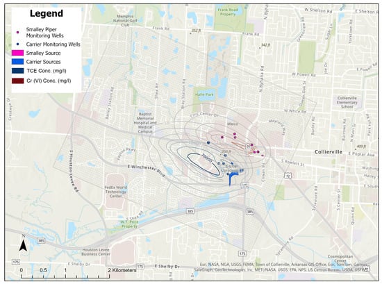
Figure 7.
TCE and Cr(VI) plume extent for the Upper Memphis Aquifer (layer-3).
A final consideration for the possible reasons mid-distance wells favored higher longitudinal dispersivities was the distribution of hydraulic conductivity that may offer a preferential flowpath between the source and certain downstream wells. Investigation of cell-to-cell hydraulic conductivity for the Carrier site did not suggest such a flowpath where values ranged between 21.09 and 22.54 m/day. Following an eight-cell connectivity, cell-to-cell changes were no greater than 0.7 m/day with the majority less than 0.5 m/day. Similarly, hydraulic conductivities along the Smalley Piper flowpath were also nominal at 22.74 to 23.18 m/day with the largest cell-to-cell change at 0.33 m/day. Therefore, no preferential flow pathways existed. Additionally, if hydraulic conductivity can serve as a proxy for changes in porosity, the ranges of conductivity do not warrant a variable field of porosities, and any model-wide increase or decrease would only shift the entire concentration field rather than impact individual arrivals of contamination to a particular well.
5. Conclusions
This study demonstrates the complexity of quantifying dispersivity in a heterogenous aquifer system with multiple sources and the importance of proper identification of source concentrations as well as contaminant data from monitoring wells. The range of dispersivity values obtained from this analysis provides several benefits over analytical or empirical values as numerical models can estimate all three dispersivity values using a minimal amount of observation data at different depths, provided having a well-calibrated flow model and known source concentration. The Memphis aquifer, although mostly confined, is threatened by anthropogenic contamination coming through the unconfined area or via preferential pathways (i.e., breaches) in the upper Claiborne confining unit [38,44,47,48], several of which are in the vicinity of municipal wellfields. Dispersivity values obtained in this study are crucial to simulating any existing or future contamination arriving at the Memphis aquifer through those breaches.
In this study, contaminant data from two U.S. EPA Superfund sites in the Town of Collierville were used to test the scale-dependent nature of longitudinal dispersivity and evaluate a range of all three dispersivity values using a three-dimensional numerical model. Source boundary conditions were defined using historical observation data near contaminant sources and dispersivity values were optimized by minimizing the root mean squared error (RMSE) between observed and simulated concentration. The following are the main conclusions from this study:
- Values of longitudinal dispersivity from the Smalley Piper and Carrier sites have the lowest values at well near the source and higher at further distances from the source.
- Dispersivities observed at wells midway and downgradient showed an increase; however, this trend was complicated by findings from the monitoring wells furthest from the sources at both sites, where dispersivities decreased below the levels observed at mid-distance wells.
- Concentration trends across all monitoring wells were generally consistent, although a few wells never reached the peak concentrations predicted by the model. The possibility of preferential flowpaths or errors in interpreting groundwater levels was considered but ultimately discounted.
- High log RMSE errors between modeled and observed concentrations at several wells were likely due to inherent inaccuracies in some of the source concentration data and a broad dispersion of observed concentrations, which made achieving a good match challenging under certain conditions.
- The Carrier site had added complexity over Smalley Piper due to it having three sources.
- Somewhat novel to this study into scale-dependent dispersivity is the presence of two plumes in the same vicinity, wherein, with a constant porosity and low-variable hydraulic conductivity field, the pattern of dispersivity changing with distance should have more closely aligned.
- Out of the thirteen monitoring wells, four had dispersivities that reached the upper limit of the likely range set by this investigation. Although an empirical equation by Gelhar (1992) [28] might suggest raising this threshold, such an adjustment could complicate matters, as it would involve increasing dispersivities for mid-distance wells, which is already problematic.
- With the threat of localized contamination elsewhere at the Memphis aquifer and not having prior knowledge of plausible values of dispersivity, this study has produced a starting range whereby longitudinal dispersivities range from 5.5 m to 20.5 m, transverse horizontal dispersivities range from 0.28 m to 3.88 m, and transverse vertical dispersivities range from 0.03 m to 0.08 m.
The results show the complexity of estimating field scale dispersivity parameters in the presence of multiple sources, multiple plumes, questionable source concentration data, and broad scatter in observed readings. Such challenges prove difficult to remedy; however, the results still offer value insights into scale-dependent dispersivity and the behavior of contaminant migration within the Memphis aquifer.
Author Contributions
Conceptualization, M.I.S. and B.W.; methodology, M.I.S.; validation, M.I.S., B.W. and F.J., formal analysis; M.I.S.; investigation, M.I.S.; resources, B.W. and S.S.; data curation, M.I.S.; writing—original draft preparation, M.I.S.; writing—review and editing, M.I.S., B.W., S.S. and F.J.; visualization, M.I.S.; supervision, B.W. and F.J.; project administration, B.W.; funding acquisition, B.W. All authors have read and agreed to the published version of the manuscript.
Funding
This study funded by Memphis Light Gas and Water (MLGW) Contract No. 12064, and supported by the Center for Applied Earth Science and Engineering Research (CAESER) at the University of Memphis.
Data Availability Statement
Access project data may be released with permission provided by the funder, Memphis Light, Gas, and Water (MLGW).
Conflicts of Interest
The authors declare no conflicts of interest regarding the publication of this paper. This research was supported by Memphis Light Gas and Water (MLGW), but the funders had no role in the design, execution, interpretation, or writing of the study.
References
- Lee, J.; Rolle, M.; Kitanidis, P.K. Longitudinal dispersion coefficients for numerical modeling of groundwater solute transport in heterogeneous formations. J. Contam. Hydrol. 2018, 212, 41–54. [Google Scholar] [CrossRef]
- Coats, K.H.; Smith, B.D. Dead-end pore volume and dispersion in porous media. Soc. Pet. Eng. J. 1964, 4, 73–84. [Google Scholar] [CrossRef]
- Chapelle, F.H. A solute-transport simulation of brackish-water intrusion near Baltimore, Maryland. Groundwater 1986, 24, 304–311. [Google Scholar] [CrossRef]
- Avon, L.; Bredehoeft, J.D. An analysis of trichloroethylene movement in groundwater at Castle Air Force Base, California. J. Hydrol. 1989, 110, 23–50. [Google Scholar] [CrossRef]
- Chiang, C.Y.; Salanitro, J.P.; Chai, E.Y.; Colthart, J.D.; Klein, C.L. Aerobic biodegradation of benzene, toluene, and xylene in a sandy aquifer—data analysis and computer modeling. Groundwater 1989, 27, 823–834. [Google Scholar] [CrossRef]
- Jensen, K.; Bitsch, K.; Bjerg, P.L. Large-scale dispersion experiments in a sandy aquifer in Denmark: Observed tracer movements and numerical analyses. Water Resour. Res. 1993, 29, 673–696. [Google Scholar] [CrossRef]
- Zou, S.; Parr, A. Two-Dimensional Dispersivity Estimation Using Tracer Experiment Data. Groundwater 1994, 32, 367–373. [Google Scholar] [CrossRef]
- Engesgaard, P.; Jensen, K.H.; Molson, J.; Frind, E.O.; Olsen, H. Large-scale dispersion in a sandy aquifer: Simulation of subsurface transport of environmental tritium. Water Resour. Res. 1996, 32, 3253–3266. [Google Scholar] [CrossRef]
- Hyndman, D.W.; Gorelick, S.M. Estimating lithologic and transport properties in three dimensions using seismic and tracer data: The Kesterson aquifer. Water Resour. Res. 1996, 32, 2659–2670. [Google Scholar] [CrossRef]
- Mallants, D.; Espino, A.; Hoorick, M.V.; Feyen, J.; Vandenberghe, N.; Loy, W. Dispersivity Estimates from a Tracer Experiment in a Sandy Aquifer. Groundwater 2000, 38, 304–310. [Google Scholar] [CrossRef]
- Schulze-Makuch, D. Longitudinal dispersivity data and implications for scaling behavior. Groundwater 2005, 43, 443–456. [Google Scholar] [CrossRef]
- Cupola, F.; Tanda, M.; Zanini, A. Laboratory Estimation of Dispersivity Coefficients. Procedia Environ. Sci. 2015, 25, 74–81. [Google Scholar] [CrossRef]
- Bai, B.; Xu, T.; Guo, Z. An experimental and theoretical study of the seepage migration of suspended particles with different sizes. Hydrogeol. J. 2016, 24, 2063–2078. [Google Scholar] [CrossRef]
- Citarella, D.; Cupola, F.; Tanda, M.G.; Zanini, A. Evaluation of dispersivity coefficients by means of a laboratory image analysis. J. Contam. Hydrol. 2015, 172, 10–23. [Google Scholar] [CrossRef] [PubMed]
- Frippiat, C.C.; Pérez, P.C.; Holeyman, A.E. Estimation of laboratory-scale dispersivities using an annulus-and-core device. J. Hydrol. 2008, 362, 57–68. [Google Scholar] [CrossRef]
- Kret, E.; Kiecak, A.; Malina, G.; Nijenhuis, I.; Postawa, A. Identification of TCE and PCE sorption and biodegradation parameters in a sandy aquifer for fate and transport modelling: Batch and column studies. Environ. Sci. Pollut. Res. 2015, 22, 9877–9888. [Google Scholar] [CrossRef] [PubMed]
- Shamir, U.Y.; Harleman, D.R.F. Numerical solutions for dispersion in porous mediums. Water Resour. Res. 1967, 3, 557–581. [Google Scholar] [CrossRef]
- Sternberg, S.P.; Cushman, J.H.; Greenkorn, R.A. Laboratory observation of nonlocal dispersion. Transp. Porous Media 1996, 23, 135–151. [Google Scholar] [CrossRef]
- Sternberg, S.P.K. Dispersion Measurements in Highly Heterogeneous Laboratory Scale Porous Media. Transp. Porous Media 2004, 54, 107–124. [Google Scholar] [CrossRef]
- Tan, C.; Tong, J.; Liu, Y.; Hu, B.X.; Yang, J.; Zhou, H. Experimental and modeling study on Cr (VI) transfer from soil into surface runoff. Stoch. Environ. Res. Risk Assess. 2016, 30, 1347–1361. [Google Scholar] [CrossRef]
- Zhang, X.; Tong, J.; Hu, B.X.; Wei, W. Adsorption and desorption for dynamics transport of hexavalent chromium (Cr (VI)) in soil column. Environ. Sci. Pollut. Res. 2018, 25, 459–468. [Google Scholar] [CrossRef] [PubMed]
- Viotti, P.; Sappa, G.; Tatti, F.; Andrei, F. nZVI Mobility and Transport: Laboratory Test and Numerical Model. Hydrology 2022, 9, 196. [Google Scholar] [CrossRef]
- Klotz, D.; Seiler, K.P.; Moser, H.; Neumaier, F. Dispersivity and velocity relationship from laboratory and field experiments. J. Hydrol. 1980, 45, 169–184. [Google Scholar] [CrossRef]
- Pickens, J.F.; Grisak, G.E. Scale-dependent dispersion in a stratified granular aquifer. Water Resour. Res. 1981, 17, 1191–1211. [Google Scholar] [CrossRef]
- Taylor, S.R.; Moltyaner, G.L.; Howard, K.W.F.; Killey, R.W.D. A comparison of field and laboratory methods for determining contaminant flow parameters. Groundwater 1987, 25, 321–330. [Google Scholar] [CrossRef]
- Dagan, G. Statistical theory of groundwater flow and transport: Pore to laboratory, laboratory to formation, and formation to regional scale. Water Resour. Res. 1986, 22, 120S–134S. [Google Scholar] [CrossRef]
- Graham, D.D. Potential for Leakage among Principal Aquifers in the Memphis Area, Tennessee; US Department of the Interior, Geological Survey: Reston, VA, USA, 1986; Volume 85.
- Gelhar, L.W.; Welty, C.; Rehfeldt, K.R. A critical review of data on field-scale dispersion in aquifers. Water Resour. Res. 1992, 28, 1955–1974. [Google Scholar] [CrossRef]
- Anderson, M.P.; Cherry, J.A. Using models to simulate the movement of contaminants through groundwater flow systems. Crit. Rev. Environ. Control 1979, 9, 97–156. [Google Scholar] [CrossRef]
- Guo, Z.; Fogg, G.E.; Brusseau, M.L.; LaBolle, E.M.; Lopez, J. Modeling groundwater contaminant transport in the presence of large heterogeneity: A case study comparing MT3D and RWhet. Hydrogeol. J. 2019, 27, 1363–1371. [Google Scholar] [CrossRef]
- Hamzaoui-Azaza, F.; Zammouri, M.; Ameur, M.; Baba Sy, M.; Gueddari, M.; Bouhlila, R. Hydrogeochemical modeling for groundwater management in arid and semiarid regions using MODFLOW and MT3DMS: A case study of the Jeffara of Medenine coastal aquifer, South-Eastern Tunisia. Nat. Resour. Model. 2020, 33, e12282. [Google Scholar] [CrossRef]
- Banaei, S.M.A.; Javid, A.H.; Hassani, A.H. Numerical simulation of groundwater contaminant transport in porous media. Int. J. Environ. Sci. Technol. 2021, 18, 151–162. [Google Scholar] [CrossRef]
- Priyanka, B.; Kumar, M.M.; Amai, M. Estimating anisotropic heterogeneous hydraulic conductivity and dispersivity in a layered coastal aquifer of Dakshina Kannada District, Karnataka. J. Hydrol. 2018, 565, 302–317. [Google Scholar] [CrossRef]
- Ansarifar, M.M.; Salarijazi, M.; Ghorbani, K.; Kaboli, A.R. Aquifer-wide estimation of longitudinal dispersivity by the combination of empirical equations, inverse solution, and aquifer zoning methods. Appl. Water Sci. 2023, 13, 14. [Google Scholar] [CrossRef]
- Konikow, L.F.; Sanford, W.E.; Campbell, P.J. Constant-concentration boundary condition: Lessons from the HYDROCOIN variable-density groundwater benchmark problem. Water Resour. Res. 1997, 33, 2253–2261. [Google Scholar] [CrossRef]
- Criner, J.H.; Parks, W.S. Historic Water-Level Changes and Pumpage from the Principal Aquifers of the Memphis Area, Tennessee: 1886–1975; Geological Survey (US): Reston, VA, USA, 1976.
- Kingsbury, J.A. Altitude of the Potentiometric Surfaces, September 1995, and Historical Water-Level Changes in the Memphis and Fort Pillow Aquifers in the Memphis Area, Tennessee; Geological Survey (US): Reston, VA, USA, 1996.
- Parks, W.S.; Carmichael, J.K. Geology and Ground-Water Resources of the Memphis Sand in Western Tennessee; Department of the Interior, US Geological Survey: Reston, VA, USA, 1990; Volume 88.
- Bradley, M.W. Ground-Water Hydrology and the Effects of Vertical Leakage and Leachate Migration on Ground-Water Quality near the Shelby County landfill, Memphis, Tennessee; US Geological Survey: Reston, VA, USA, 1991.
- Parks, W.S.; Mirecki, J.E.; Kingsbury, J.A. Hydrogeology, Ground-Water Quality, and Source of Ground Water Causing Water-Quality Changes in the Davis Well Field at Memphis, Tennessee; US Department of the Interior, US Geological Survey: Reston, VA, USA, 1995; Volume 94.
- Carmichael, J.K. Hydrogeology and Ground-Water Quality at Naval Support Activity Memphis, Millington, Tennessee; US Department of the Interior, US Geological Survey: Reston, VA, USA, 1997; Volume 97.
- Larsen, D.; Gentry, R.W.; Ivey, S.; Solomon, D.K.; Harris, J. Groundwater leakage through a confining unit beneath a municipal well field, Memphis, Tennessee, USA. In Proceedings of the Geochemical Processes in Soil and Groundwater: Measurement, Modelling, Upscaling. GeoProc2002 Conference, Bremen, Germany, 4–7 March 2002; Wiley-VCH Verlag GmbH: Weinheim, Germany, 2003; pp. 51–64. [Google Scholar]
- Clark, B.R.; Hart, R.M. The Mississippi Embayment Regional Aquifer Study (MERAS): Documentation of a Groundwater-Flow Model Constructed to Assess Water Availability in the Mississippi Embayment; Technical Report; U. S. Geological Survey: Reston, VA, USA, 2009.
- Waldron, B.A.; Harris, J.B.; Larsen, D.; Pell, A. Mapping an aquitard breach using shear-wave seismic reflection. Hydrogeol. J. 2009, 17, 505. [Google Scholar] [CrossRef]
- Ge, J.; Magnani, M.B.; Waldron, B. Imaging a shallow aquitard with seismic reflection data in Memphis, Tennessee, USA. Part I: Source comparison, walk-away tests and the plus-minus method. Near Surf. Geophys. 2010, 8, 331–340. [Google Scholar] [CrossRef]
- Carmichael, J.K.; Kingsbury, J.A.; Larsen, D.; Schoefernacker, S. Preliminary Evaluation of the Hydrogeology and Groundwater Quality of the Mississippi River Valley Alluvial Aquifer and Memphis Aquifer at the Tennessee Valley Authority Allen Power Plants, Memphis, Shelby County, Tennessee; Technical Report; US Geological Survey: Reston, VA, USA, 2018.
- Jazaei, F.; Waldron, B.A.; Schoefernacker, O.; Larsen, D. Numerical tools for identifying confining unit breaches impacting semi-confined water-supply aquifers. In AGU Fall Meeting Abstracts; American Geophysical Union: Washington, DC, USA, 2018; Volume 2018, p. H41J–2212. [Google Scholar]
- Torres-Uribe, H.E.; Waldron, B.; Larsen, D.; Schoefernacker, S. Application of Numerical Groundwater Model to Determine Spatial Configuration of Confining Unit Breaches near a Municipal Well Field in Memphis, Tennessee. J. Hydrol. Eng. 2021, 26, 05021021. [Google Scholar] [CrossRef]
- Moore, G.K.; Brown, D.L. Stratigraphy of the Fort Pillow Test Well, Lauderdale County, Tennessee; Tennessee Department of Conservation, Division of Geology: Nashville, TN, USA, 1969.
- Van Arsdale, R.; Bresnahan, R.; McCallister, N.; Waldron, B. Upland Complex of the central Mississippi River valley: Its origin, denudation, and possible role in reactivation of the New Madrid seismic zone. In Continental Intraplate Earthquakes: Science, Hazard, and Policy Issues; US Geological Survey: Reston, VA, USA, 2007. [Google Scholar]
- Robinson, J.L. Hydrogeologic Framework and Simulation of Ground-Water Flow and Travel Time in the Shallow Aquifer System in the Area of Naval Support Activity Memphis, Millington, Tennessee; US Department of the Interior, US Geological Survey: Reston, VA, USA, 1997; Volume 97.
- Gentry, R. Novel Techniques for Investigating Recharge to the Memphis Aquifer; American Water Works Association: Denver, CO, USA, 2006. [Google Scholar]
- Waldron, B.; Larsen, D.; Hannigan, R.; Csontos, R.; Anderson, J.; Dowling, C.; Bouldin, J. Mississippi Embayment Regional Ground Water Study; United States Environmental Protection Agency: Washington, DC, USA, 2011; Volume 600.
- Parks, W.S. Hydrogeology and Preliminary Assessment of the Potential for Contamination of the Memphis Aquifer in the Memphis Area, Tennessee; Report 90-4092; Department of the Interior, US Geological Survey: Reston, VA, USA, 1990. [CrossRef]
- Black & Veatch Special Projects Corp, Groundwater Implementation Status Report 2; For the Groundwater Sampling Event, November 2016; Technical Report 2; Smalley-Piper Superfund Site Collierville: Shelby County, TN, USA, 2017.
- Black & Veatch Special Projects Corp. Remedial Action Report, Smalley-Piper Site; Technical Report; US Geological Survey: Reston, VA, USA, 2014.
- Agency for Toxic Substances and Disease Registry (ATSDR). Hazardous Substances Emergency Events Surveillance (HSEES) Annual Report 2006. Available online: https://www.atsdr.cdc.gov/HS/HSEES/annual2006.pdf (accessed on 6 December 2023).
- Hasan, K. Investigation of Modern Leakage Based on Numerical and Geochemical Modeling Near a Municipal Well Field in Memphis, Tennessee. Ph.D. Thesis, The University of Memphis, Memphis, TN, USA, 2023. [Google Scholar]
- Villalpando-Vizcaino, R.; Waldron, B.; Larsen, D.; Schoefernacker, S. Development of a numerical multi-layered groundwater model to simulate inter-aquifer water exchange in Shelby County, Tennessee. Water 2021, 13, 2583. [Google Scholar] [CrossRef]
- Sahagún-Covarrubias, S.; Waldron, B.; Larsen, D.; Schoefernacker, S. Characterization of hydraulic properties of the Memphis Aquifer by conducting pumping tests in active well fields in Shelby County, Tennessee. JAWRA J. Am. Water Resour. Assoc. 2022, 58, 185–202. [Google Scholar] [CrossRef]
- Schrader, T. Potentiometric Surface in the Sparta-Memphis Aquifer of the Mississippi Embayment; U.S. Geological Survey Scientific Investigations Map 3014; Technical Report; U.S. Geological Survey: Reston, VA, USA, 2007.
- Niswonger, R.G.; Panday, S.; Ibaraki, M. MODFLOW-NWT, A Newton formulation for MODFLOW-2005; Report 6-A37; U.S. Geological Survey: Reston, VA, USA, 2011. [CrossRef]
- Brantley, B. United Technologies Corporation, Carrier Air Conditioning Collierville, Tennessee; Supplemental Investigation Report; U.S. Geological Survey: Reston, VA, USA, 2017.
- Larsen, D.; Brock, C.F. Sedimentology and petrology of the Eocene Memphis Sand and younger terrace deposits in surface exposures of western Tennessee. Southeast. Geol. 2014, 50, 193–214. [Google Scholar]
- Lumsden, D.N.; Hundt, K.R.; Larsen, D. Petrology of the Memphis Sand in the northern Mississippi Embayment. Southeast. Geol. 2009, 46, 121–133. [Google Scholar]
- Antonacci, T.; Lee, E.S.; Kim, Y. Characterizing and predicting contaminant transport in the Newport Wellfield aquifer, Ohio. Geosci. J. 2013, 17, 465–477. [Google Scholar] [CrossRef]
- Rai, D.; Eary, L.E.; Zachara, J.M. Environmental chemistry of chromium. Sci. Total Environ. 1989, 86, 15–23. [Google Scholar] [CrossRef] [PubMed]
- Leaf, A.T.; Fienen, M.N. Flopy: The Python Interface for MODFLOW. Groundwater 2022, 60, 710–712. [Google Scholar] [CrossRef] [PubMed]
- Zheng, C.; Wang, P.P. MT3DMS: A Modular Three-Dimensional Multispecies Transport Model for Simulation of Advection, Dispersion, and Chemical Reactions of Contaminants in Groundwater Systems; Documentation and User’s Guide; U.S. Army Engineer Research and Development Center, Environmental Laboratory: Vicksburg, MI, USA, 1999. [Google Scholar]
- Xu, M.; Eckstein, Y. Use of Weighted Least-Squares Method in Evaluation of the Relationship Between Dispersivity and Field Scale. Groundwater 1995, 33, 905–908. [Google Scholar] [CrossRef]
- Environmental and Safety Designs, Inc. Carrier Corporation Site Investigation Report; Site Investigation: Memphis, TN, USA, 1988; Volume 1. [Google Scholar]
- Waldron, B.; Larsen, D. Pre-Development Groundwater Conditions Surrounding Memphis, Tennessee: Controversy and Unexpected Outcomes. JAWRA J. Am. Water Resour. Assoc. 2015, 51, 133–153. [Google Scholar] [CrossRef]
- Lozano-Medina, D.; Waldron, B.; Schoefernacker, S.; Antipova, A.; Villalpando-Vizcaino, R. Stories of a water-table: Anomalous depressions, aquitard breaches and seasonal implications, Shelby County, Tennessee, USA. Environ. Monit. Assess. 2023, 195, 953. [Google Scholar] [CrossRef]
- Sloto, R. Changes in Groundwater Flow and Volatile Organic Compound Concentrations at the Fischer and Porter Superfund Site, Warminster Township, Bucks County, Pennsylvania, 1993–2009; US Geological Survey: Reston, VA, USA, 2010.
- Zech, A.; Attinger, S.; Bellin, A.; Cvetkovic, V.; Dagan, G.; Dietrich, P.; Fiori, A.; Teutsch, G. Evidence based estimation of macrodispersivity for groundwater transport applications. Groundwater 2023, 61, 346–362. [Google Scholar] [CrossRef]
Disclaimer/Publisher’s Note: The statements, opinions and data contained in all publications are solely those of the individual author(s) and contributor(s) and not of MDPI and/or the editor(s). MDPI and/or the editor(s) disclaim responsibility for any injury to people or property resulting from any ideas, methods, instructions or products referred to in the content. |
© 2024 by the authors. Licensee MDPI, Basel, Switzerland. This article is an open access article distributed under the terms and conditions of the Creative Commons Attribution (CC BY) license (https://creativecommons.org/licenses/by/4.0/).