Performance Evaluation of Regression-Based Machine Learning Models for Modeling Reference Evapotranspiration with Temperature Data

Abstract

In this study, due to their flexibility in forecasting, the capabilities of three regression-based machine learning models were explored, specifically random forest regression (RFr), generalized regression neural network (GRNN), and support vector regression (SVR). The above models were assessed for their suitability in modeling daily reference evapotranspiration (ET_o), based only on temperature data (T_min, T_max, T_mean), by comparing their daily ET_o results with those estimated by the conventional FAO 56 PM model, which requires a broad range of data that may not be available or may not be of reasonable quality. The RFr, GRNN, and SVR models were subjected to performance evaluation by using statistical criteria and scatter plots. Following the implementation of the ET_o models’ comparisons, it was observed that all regression-based machine learning models possess the capability to accurately estimate daily ET_o based only on temperature data requirements. In particular, the RFr model outperformed the others, achieving the highest R value of 0.9924, while the SVR and GRNN models had R values of 0.9598 and 0.9576, respectively. Additionally, the RFr model recorded the lowest values in all error metrics. Once these regression-based machine learning models have been successfully developed, they will have the potential to serve as effective alternatives for estimating daily ET_o, under current and climate change conditions, when temperature data are available. This information is crucial for effective water resources management and especially for predicting agricultural production in the context of climate change.

1. Introduction

The decrease in water availability over the last few decades is one of the principal environmental problems that could severely restrict agricultural production and industrial development in some arid and semiarid areas of the world [1,2], particularly under climate change conditions. Evapotranspiration (ET) is a parameter of major importance, participating in both hydrological cycle and surface energy balance [1,2,3], and is well-established in various disciplines such as hydrology [4], agronomy [5], climatology [6], and other geosciences [7]. Modeling daily reference evapotranspiration (ET_o) holds significant importance in various aspects, including water resources management, estimating water balances, scheduling irrigation, forecasting agricultural production, and addressing theoretical challenges within the fields of hydrology and meteorology. The ASCE-standardized method [8], at a daily step for short reference crops (clipped grass of 0.12 m), gives, as suggested by [8], equivalent ET_o results to the FAO56 Penman–Monteith (FAO 56 PM) equation [9]. The FAO 56 PM equation was adopted by the FAO as a standard method of estimating ET_o, as it gives more consistent ET_o estimates, and it has been shown to perform better than other ET_o methods [8,9]. However, the detailed meteorological data required by the FAO 56 PM equation are not often available, especially in developing countries. In such circumstances, there is much research for innovative modeling approaches to ensure the trustworthy estimation of ET_o values.

In recent years, artificial intelligence (AI), including machine learning (ML) modeling techniques, has gained significant popularity for estimating and forecasting purposes across various domains, including water resources and environmental science [1,2,3,4,5,6,7,8,9]. Since the early 2000s, there have been discussions about machine learning concepts and applications in hydrology.

The ASCE Task Committee [10] recognized artificial neural networks (ANNs) as a reliable modeling tool, prompting the further exploration of machine learning (ML) techniques in various hydrological and climatological applications. Since then, ML methods have been used for water quality examination, hydrologic time series analysis [11,12,13,14,15], landslide susceptibility mapping [16], and climate impact assessments on dam seepage [17].

Several studies have focused on estimating reference evapotranspiration (ET_o) using ML techniques. For example, ref. [18] used a cascade correlation neural network with Kalman filtering for monthly ET_o estimation, while [19] found that generalized regression neural networks (GRNNs) outperformed radial basis function neural networks (RBFNNs) for daily ET_o estimation in northern Algeria. Similarly, ref. [20] evaluated least square support vector regression, multivariate adaptive regression splines, and M5 Model Tree for ET_o estimation. Ref. [21] explored daily ET_o estimation using ANNs and empirical equations with limited input data, and [22] proposed GRNN and random forest models for daily ET_o in the Sichuan basin, southwest China.

Various studies have explored the use of boosted machine learning models as alternatives to empirical methods for estimating daily reference evapotranspiration (ET_o). For instance, ref. [23] investigated boosted ML models, while [24] examined spatial and temporal ML approaches for ET_o estimation. Linear regression algorithms were explored by [25] using limited climate data, and [26] focused on support vector machine (SVM) models for reference crop evapotranspiration. A comprehensive evaluation of ML models at both general and regional levels was conducted by [27]. In an arid climate context, ref. [28] assessed the performance of ML algorithms for ET_o estimation. Lastly, ref. [29] explored the k-nearest neighbor algorithm, multigene genetic programming, and support vector regression (SVR) for daily ET_o estimation in Turkey.

The literature mentioned above highlights the necessity for further investigation into the capabilities of different machine learning algorithms and structures. Nevertheless, the utilization of machine learning algorithms and their various adaptations in water resources applications have not been fully exploited. Towards this direction, the main objective of this study is to investigate and finally evaluate three regression-based machine learning modeling approaches, namely random forest regression (RFr), generalized regression neural network (GRNN) and support vector regression (SVR), for accurate and reliable daily reference evapotranspiration (ET_o) estimation. The difference between this work and the Hargreaves–Samani (HG-S) method [30,31], which also assesses temperature-based features for the estimation of ET_o, is examined. Taking advantage of the capabilities offered by the strength of machine learning, the goal was to construct accurate daily ET_o prediction models using only temperature data (T_min, T_max, T_mean) and astronomical data (extraterrestrial radiation (R_a), and theoretical sunshine (N), which can easily be estimated for a certain day and location) as inputs. It is important to mention that machine learning models built based on temperature can also be extended to predict ET_o using predicted temperature data, especially in the context of climate change conditions.

The motivation for employing the RFr, GRNN, and SVR machine learning approaches was to evaluate various algorithmic strategies for the same problem using three distinct modeling techniques, thereby aiming to produce the most reliable results possible. The reasoning behind the selection of these algorithms was that RFr is an ensemble learning algorithm that leverages the combined knowledge of multiple models to enhance overall performance. GRNN is a probabilistic neural network, which offers significant advantages, particularly its ability to efficiently converge to the underlying data function even with a limited number of training samples. Finally, the ε-SVR methodology addresses the nonlinear regression problem by transforming it into a linear one using kernel functions.

The performance evaluation of the RFr, GRNN and SVR models was assessed by comparing their daily ET_o results with those of the FAO 56 PM model [8,9], while the data we used were obtained from daily meteorological data collected at two weather stations, which are sited at Sindos and Piperia, in northern Greece. These stations were selected because they are located in regions frequently affected by droughts due to the combined influence of climate change and extensive human activities. Additionally, this work is motivated by the fact that, so far, scientists in Greece have not investigated the use of machine learning models with temperature-based features. Furthermore, there is a scarcity of global evaluations of these three specific methodologies using only temperature measurements.

2. Materials and Methods

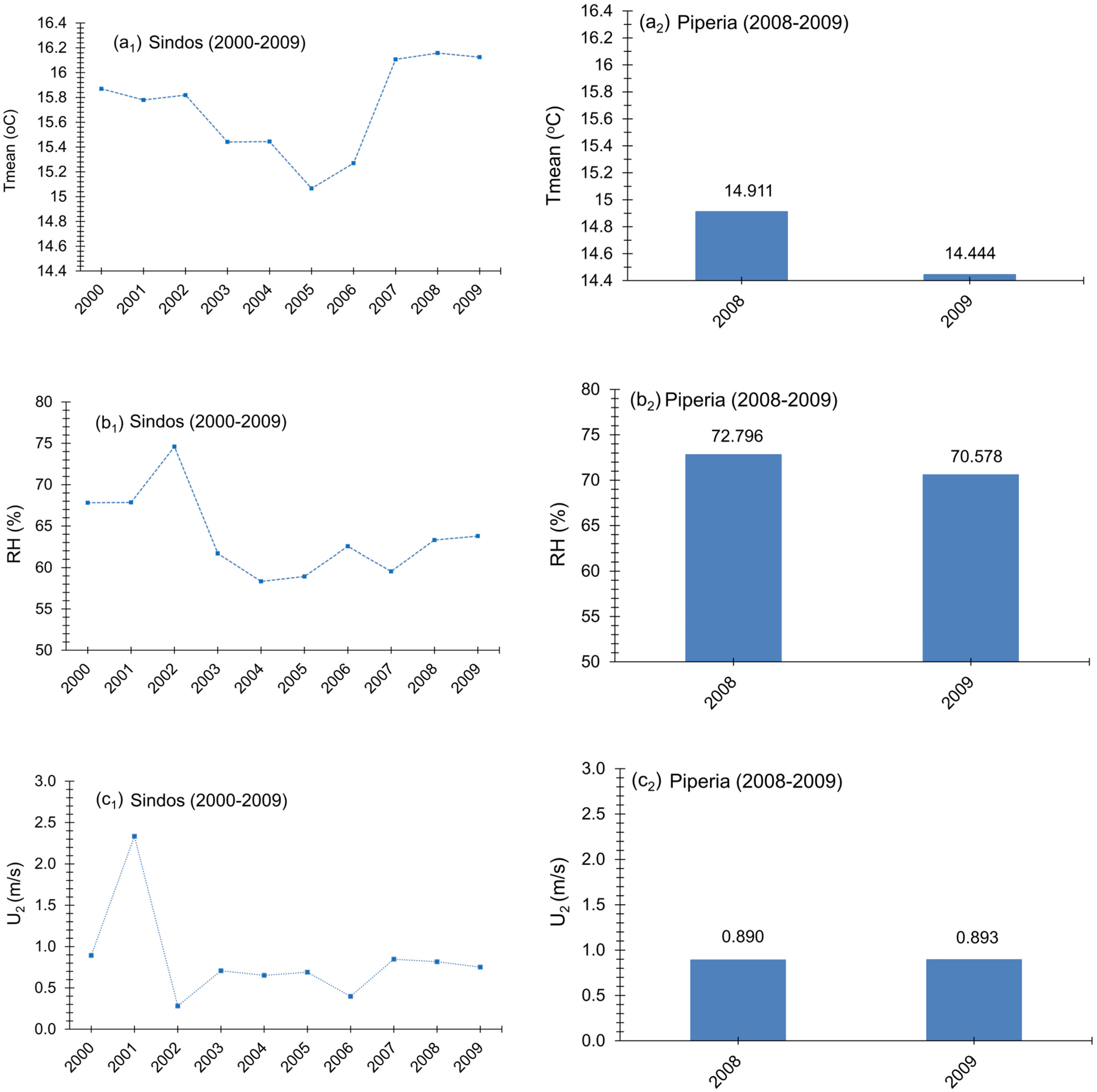
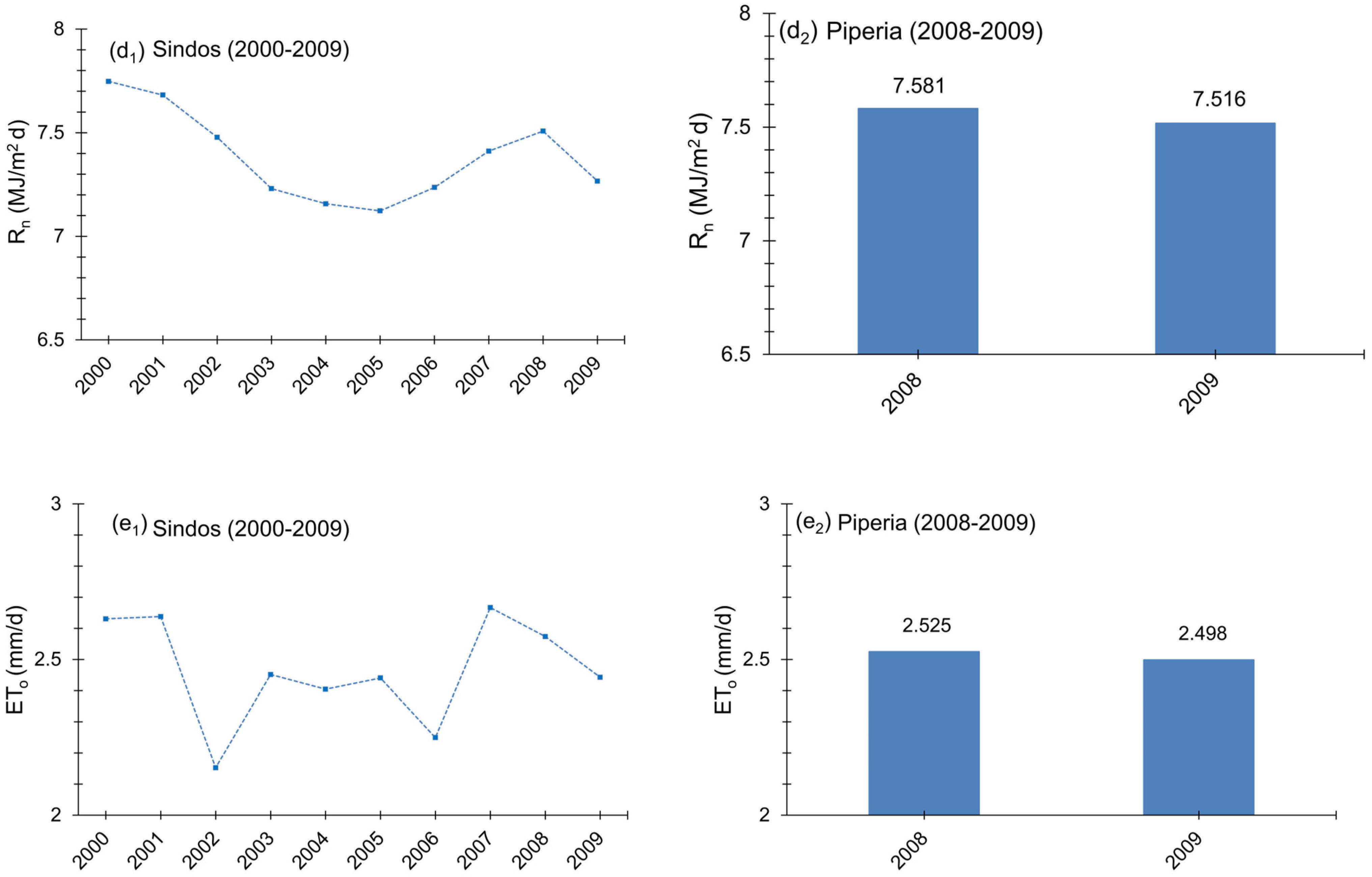
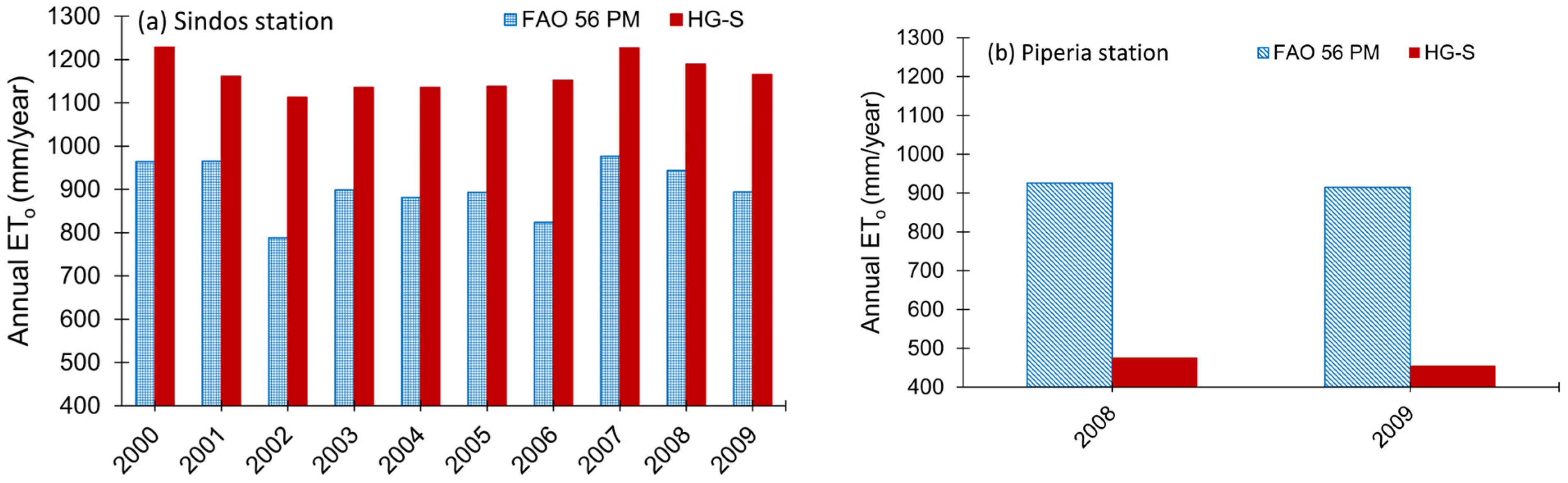
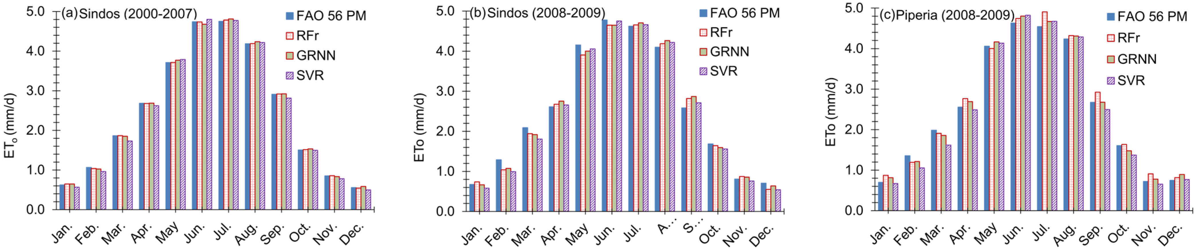
2.1. Study Area and Data

The study area is located in northern Greece. Daily meteorological variables, including maximum (T_max)/minimum (T_min) air temperature at 2 m height, mean relative humidity (RH), wind speed at 2 m height (U₂), and net solar radiation (R_n), were obtained at Sindos meteorological station (Lat. 40°41′, Lon. 22°47′, Alt. 10 m), with 2000–2007 as the training period and 2008–2009 as the testing period. The daily data from Piperia station (Lat. 40°58′, Lon. 22°00′, Alt. 160 m) (Figure 1) were used as a separate testing period during the years 2008–2009. Mean air temperature (T_mean) was estimated by averaging T_min and T_max.

Figure 2 and Figure 3 present the monthly and inter-annual variation in meteorological variables (mean air temperature, relative humidity, wind speed, net solar radiation, and reference evapotranspiration estimated using the FAO 56 PM method (Equation (1)).

These variations are shown for Sindos station during the test periods 2000–2007 and 2008–2009 and for Piperia station during the test period 2008–2009. Since the models operate on a daily time step, the mean monthly temperature values do not capture the deviations in daily values, which can reach up to 12.5 °C, with lower temperatures typically observed at Piperia station (alt. 160 m) compared to Sindos station (alt. 10 m). However, the mean monthly temperature values in Figure 2a and the mean annual temperature values in Figure 3(a₁,a₂) clearly show temperature disparities between the two stations. Additionally, Figure 2 and Figure 3 indicate notable differences in relative humidity and wind speed between the stations.

2.2. FAO56 Penman–Monteith (FAO 56 PM) Method

In this study, the performance of the RFr, GRNN, and SVR models, using only temperature data (T_min, T_max, T_mean) and astronomical data (extraterrestrial radiation (R_a) and theoretical sunshine (N)) as inputs, was assessed by comparing their daily ET_o results with those of the conventional FAO 56 PM method. This method was adopted by the FAO as the standard method of estimating ET_o as it gives more consistent ET_o estimates, and it has been shown to perform better than other ET_o methods [8,9]. According to [8,9], the FAO 56 PM method is summarized by the following equation:

$${ET}_o=\left[0.408 \left(R_n-G\right)+\gamma \frac{900}{{\rm T}+273} U_{2 }\left(e_s-e_a\right)\right]/\left[\mathsf{\Delta }+\gamma \left(1+0.34 U_2\right)\right]$$

(1)

where ET_o is the reference evapotranspiration (mm d⁻¹), R_n is the daily net solar radiation (MJ m⁻² d⁻¹), G is the soil heat flux (MJ m⁻² d⁻¹), T is the average daily air temperature at a height of 2 m (°C), U₂ is the daily mean of the wind speed at a height of 2 m (m s⁻¹), e_s is the saturation vapor pressure (kPa), e_a is the actual vapor pressure (kPa), Δ is the slope of the saturation vapor pressure versus the air temperature curve (kPa °C⁻¹), and γ is the psychrometric constant (kPa °C⁻¹). All parameters were calculated using equations provided by [9]. The soil heat flux (G) was assumed to be zero over the calculation time step period (24 h) [8].

Extraterrestrial radiation (R_a) and theoretical sunshine (N), which are astronomical data, can easily be estimated for a certain day and location, according to [9], as follows:

$$R_a=\frac{24 \left(60\right)}{\pi } G_{sc} d_r \left[{\omega }_{s }sin\left(\phi \right) sin\left(\delta \right)+cos\left(\phi \right) cos\left(\delta \right) sin\left({\omega }_s\right) \right]$$

(2)

$$N=\frac{24}{\pi } {\omega }_s$$

(3)

where R_a is extraterrestrial radiation (MJ/m² d), G_sc is the solar constant (0.0820 MJ/m² min), d_r is the inverse relative distance between the Earth and the Sun, ω_s is the sunset hour angle (rad), φ is latitude (rad), δ is solar declination (rad), and N is theoretical sunshine (h).

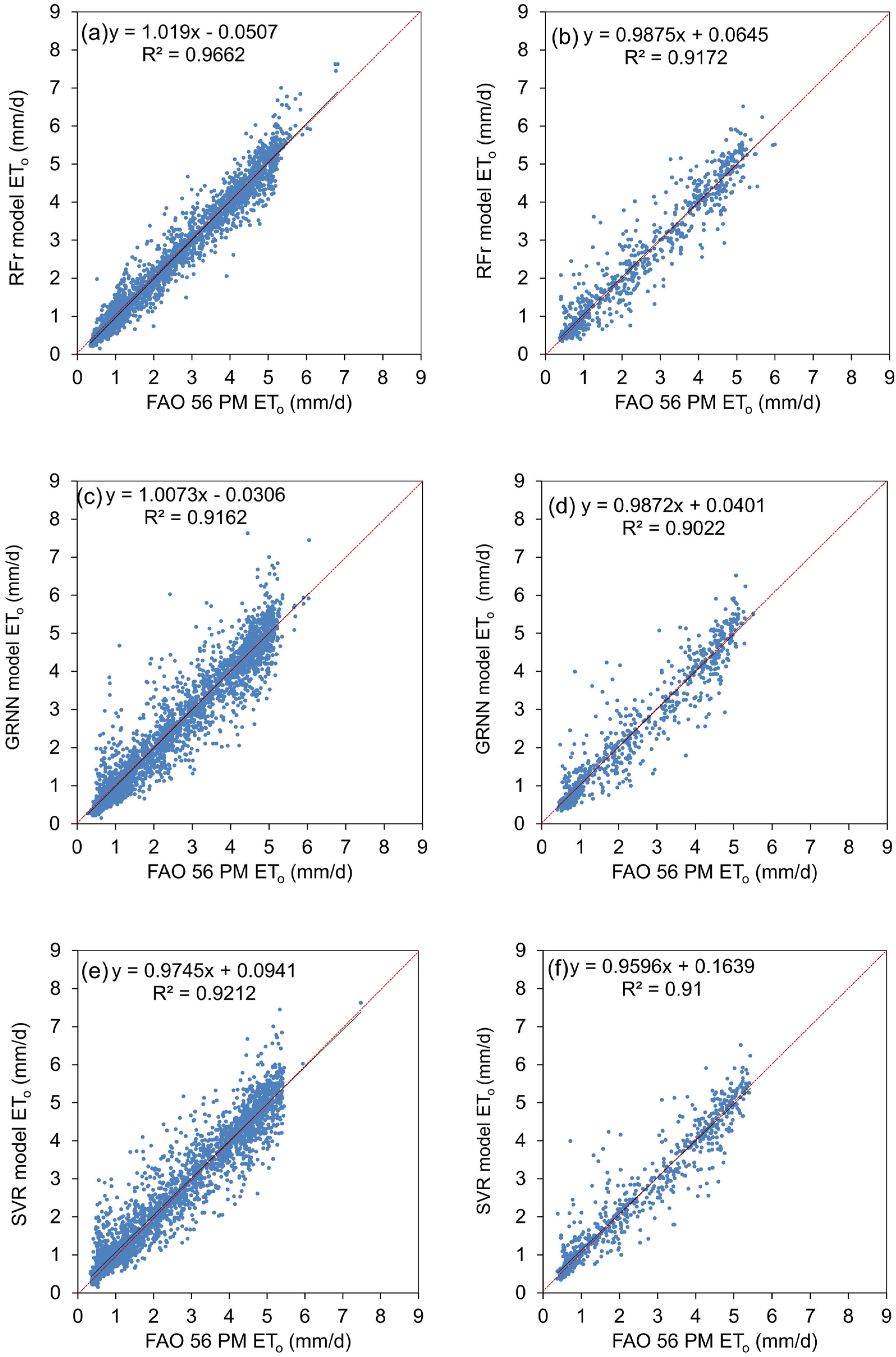
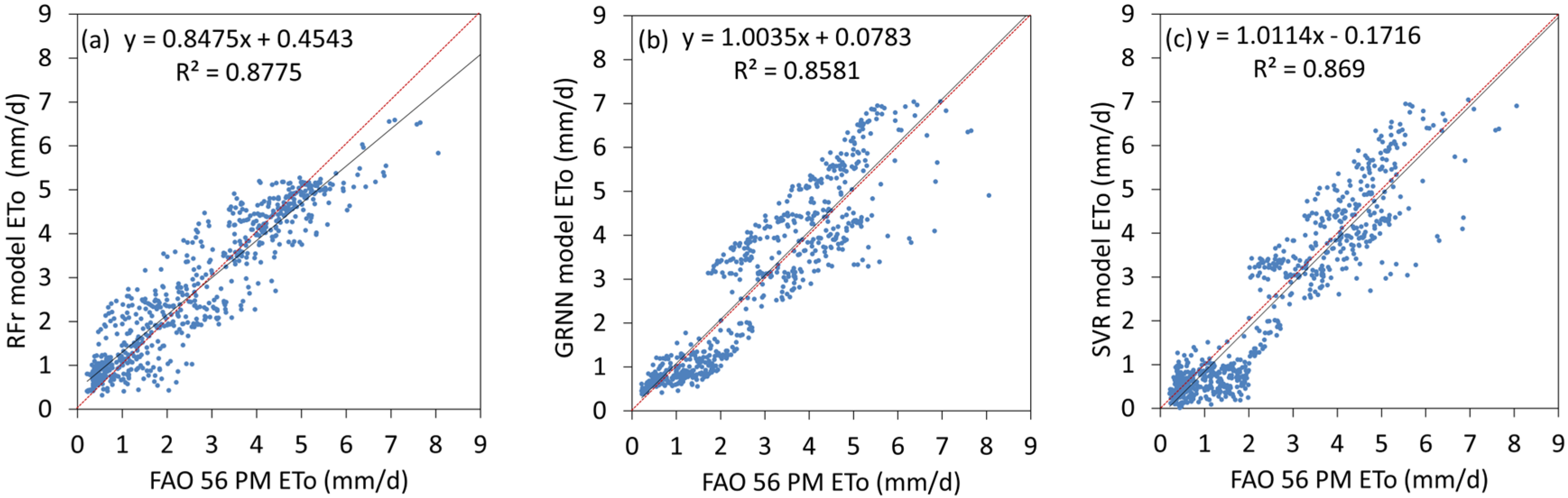
2.3. Machine Learning Modeling Approaches

Partitioning the dataset into distinct training and testing subsets constitutes a foundational procedure in machine learning, enabling efficient model training, performance assessment, and protection against overfitting. This methodology serves to promote the model’s ability to effectively generalize to unseen data and make precise predictions in practical real-world applications. Due to this fact, the available dataset was divided into two parts: the daily meteorological data for the period 2000–2007 as the fitting dataset and the daily meteorological data for the period 2008–2009 as the test dataset from Sindos station. In order for the predictive ability of the built machine learning models to be further assessed, the daily meteorological data for the period 2008–2009 from the Piperia station were used as a second test dataset as well. The k = 10 cross-validation technique [32] was applied to the comprehensive dataset, consisting of 2922 daily measurements, ensuring that all available data patterns were taken into account during the model construction phase.

• Random Forest for regression (RFr)

Utilizing the structural and algorithmic power of machine learning techniques, which are known for their superiority in simulating intricate non-linear systems, and, considering the fact that as non-parametric methods, they can bypass the constraints of standard regression modeling [33], the random forest for regression (RFr) machine learning modeling approach was employed in order for accurate and reliable ET_o models to be created. This modeling technique has been extensively described in [34]. Ref. [35] was the pioneer in introducing this supervised machine learning technique, founded on the idea that multiple models have the capacity to generate an outcome capable of capturing the true underlying structure of the available data. Random forest for regression (RFr) utilizes numerous individual models, known as decision trees, which are ultimately aggregated into one, aiming to minimize both the variance and bias of the base learner, which is the decision tree, to the greatest extent achievable by the system. This approach, referred to as ensemble learning [36,37,38], harnesses the combined knowledge of multiple models to enhance the overall performance of the learning system. That is, a random forest comprises a collection of regression trees (decision trees), utilizing their information collectively.

In the training process, the observations within the fitting dataset are employed to create numerous regression trees, each having distinct training parameters, thereby contributing uniquely to the prediction process. The ultimate observation prediction results from the amalgamation of all individual predictions, thereby leveraging the diverse internal characteristics of each tree to improve generalization. It represents a form of decision structure learning, centered on a predictive model, with the aim of accurately estimating the dependent variable based on the observed values of independent variables.

Each individual regression tree comprises a connected flowchart. In this structure, there is a solitary starting node from which two branches initially extend and lead to ‘child’ nodes stemming from their parent nodes. Each node has a specific satisfaction condition (impurity criterium), and if this objective is not met, the process advances to a new node and its corresponding children. The ensemble method used for ET_o model construction was bootstrapped aggregation (bagging) [36,39,40,41,42,43]. This approach entails training multiple independent models on random subsets (bootstraps) of the fitting data. The algorithm selects a random subset of the available features while ensuring there is no correlation among the decision tree estimators. These estimators showed, as expected, high variance, since they perfectly capture the pattern of the particular sample data. Ultimately, when the predictions from these individual models (regression trees) were combined through averaging, the variance in aggregation was significantly reduced.

For the development of a precise and reliable RFr model, it is essential to appropriately adjust its learning hyperparameters. The most critical factors in this process are the quantity of decision trees and their maximum depth within the modeling system. Additionally, careful consideration should be given to parameters such as the minimum number of samples necessary to split a node, the minimum number of samples required for a leaf node, and the number of features to be considered when searching for the optimal split. To identify the most suitable combination of hyperparameters for the RFr model, we utilized a trial-and-error approach, aiming to minimize the mean square error. This involved iterating through various settings for the first two hyperparameters, while keeping the last three at their default values, until we achieved the desired target error. We examined a range of values for the number of decision trees and their maximum depth, spanning from 50 to 500 per unit for the former and 5 to 12 per unit for the latter. The default values for the minimum number of samples required to split a node, the minimum number of samples needed for a leaf node, and the number of features considered for the optimal split were 2, 1, and 1, respectively.

• Generalized Regression Neural Network (GRNN)

The utilization of a probabilistic neural network, such as a GRNN, offers significant benefits, primarily because it can efficiently converge towards the underlying data function even when there are limited training samples available. Moreover, the minimal additional knowledge required for achieving a satisfactory fit can be obtained without requiring further input from the user. Consequently, this makes the generalized regression neural network (GRNN) a highly valuable tool for making predictions and conducting practical comparisons of system performance. As a statistical method of function approximation into the structure of a neural network, generalized regression neural networks (GRNNs) [44] have been successfully used for daily reference evapotranspiration modeling [20,22,45,46]. The concluding remarks of the conducted research indicate that this artificial neural network methodology is worthy of further exploration in hydrology studies. GRNNs have been described extensively in the related literature [47,48,49]. Summarizing, the learning of this methodology depends on a single parameter (σ), which is known as the smoothing parameter. It represents the width of the normalized Gaussian function which is embedded in the probability density function used in single-bandwidth GRNN training and can be described as follows:

$$\widehat{Y}(X)=\frac{\sum _{i=1}^n{Y}_i\exp \left(-\frac{{(X-X_i)}^T·(X-X_i)}{2·{\sigma }^2}\right)}{\sum _{i=1}^n\exp \left(-\frac{{(X-X_i)}^T·(X-X_i)}{2·{\sigma }^2}\right)}$$

(4)

where $\widehat{Y}(X)$ represents the Nadaraya–Watson kernel regression estimator; $\mathit{exp} \left(-\frac{\sum _{i=1}^n{\left(X-X_i\right)}^T·\left(X-X_i\right)}{2·{\sigma }^2}\right)$ is the Gaussian radial basis function (RBF), whose outcome is influenced by the smoothing parameter (σ) value; X is the current input vector and X_i is the corresponding training output vector; n is the number of elements of the vector X; and the symbol T represents the transpose operation applied to the vector.

A CRNN’s architecture comprises four distinct layers. The initial layer functions as the input layer, where independent variables are introduced to the system. Subsequently, a second layer called the pattern layer is established, which receives information from the input layer. Within the pattern layer, each node generates a signal using the RBF (radial basis function) and transmits it to the next layer, known as the summation layer, which is the third layer. In this layer, $\sum _{i=1}^n{\left(X-X_i\right)}^T·\left(X-X_i\right)$ represents the squared Euclidean distance between the training value and the prediction point, serving as a gauge of the neural network’s adaptation to the actual training values. Finally, the fourth layer, known as the output layer, incorporates the values obtained from Equation (4).

Based on the preceding explanation, it becomes obvious that the precise choice of the smoothing coefficient (σ) is of outmost importance for both the accuracy and generalization capability of the final GRNN model. Therefore, its value was fine-tuned using an exhaustive grid-search method [50] through a trial-and-error process, spanning the range of [0, 10] with increments of 0.001. This selection was driven by optimizing a combination of maximum correlation and minimum mean square error between the observed values and those estimated by the GRNN model.

• Support Vector Regression (SVR)

Support vector regression (SVR) is another highly promising algorithm within the realm of machine learning approaches, offering considerable potential for application in environmental modeling. It was initially introduced along with the concept of the capacity of machine learning by [51], in conjunction with the work of Cortes and Vapnik [52]. A comprehensive description of SVR can be found in Vapnik’s works from 1999 and 2000 [53,54], as well as in the publications [55,56]. In essence, this methodology addresses the nonlinear regression problem by converting it into a linear one through the use of kernel functions. To achieve this transformation via the ε-SVR algorithm, the original input space is mapped onto a higher-dimensional feature space. ε-SVR involves the creation of an initial space with a width of (2ε), where ε > 0, effectively encapsulating the original data within the range [−ε, +ε]. With the introduction of an additional variable ξ_i, referred to as a slack variable, which quantifies the deviation of each training point from the initial space with a width of (2ε), the system aims to minimize the ε-insensitive loss function [54,56,57]:

$$min\frac{1}{2}{‖w‖}^2+C·{\sum }_{i=1}^n\left({\xi }_i^{+}+{\xi }_i^{-}\right) \mathrm{subject} \mathrm{to} \left\{\begin{array}{c}{y}_i-w^T\phi \left(x_{i }\right)-bc \le \epsilon +{\xi }_i^{+}\\ y_i-w^T\phi \left(x_{i }\right)-bc \le -\epsilon -{\xi }_i^{-}\\ {\xi }_i^{+},{\xi }_i^{-}\ge 0, i=1, \dots , n\end{array}\right.$$

(5)

where C is a system’s hyperparameter that needs to be tuned, w is the vector of the weights, and bc is the system’s bias.

Out of the four kernel functions offered in ε-SVR, which include the radial basis function, linear, sigmoid, and polynomial, the radial basis function (RBF) kernel (Equation (6)) was chosen for its capacity to effectively measure similarity. It was employed to convert the data into a multi-dimensional super-space (m-dimensional) with the aim of representing intricate nonlinear relationships using an optimal straight line:

$$K\left(x_i-x_j\right)=\exp \left(-\gamma {‖x_i-x_j‖}^2\right), \gamma >0$$

(6)

where $\gamma =\left(\raisebox{1ex}{$1$}\!\left/ \!\raisebox{-1ex}{${2\sigma }^2$}\right.\right)$, and $‖x_i-x_j‖$ is the Euclidean distance between the support vectors (SVs).

Considering Equations (5) and (6), it can be seen that the precision of estimation and the intricacy of ε-SVR models rely on three key hyperparameters. These include (ε), responsible for determining the width of the ε-insensitive zone; gamma (γ), serving as the tuning parameter for Gaussian radial basis function (RBF) kernels; and the cost parameter (C), which regulates the influence of each support vector, effectively managing the trade-off between misprediction and model simplicity. The optimal combination of these hyperparameters was determined through an exhaustive grid-search approach [50], where (ε) varied between 0.01 and 0.8 in increments of 0.01, (γ) ranged from 0.01 to 1 with steps of 0.01, and (C) spanned from 1 to 100 in increments of 1.

All machine learning modeling methodologies used were implemented using the scikit-learn libraries [58] within the Python programming language [59].

2.4. Performance Evaluation Criteria

In order to determine the accuracy in modeling daily reference evapotranspiration of the RFr, GRNN and SVR models employed in this study, graphical and numerical analyses of the errors were performed. For this purpose, four different criterium values were used. These evaluation metrics are the correlation coefficient (R, mm/d), the absolute average error (AAE, mm/d), the root mean square error (RMSE, mm/d), and the percent relative error (RE%). The formulas for these metrics are provided below:

$$R=\frac{{\sum }_{i=1}^n\left({ET}_i^{PM}-\overline{{ET}_i^{PM}}\right)·\left({ET}_i^M-\overline{{ET}_i^M}\right)}{\sqrt{\left(\sum _{i=1}^n{\left({ET}_i^{PM}\right)}^2-\frac{{\left(\sum _{i=1}^n{ET}_i^{PM}\right)}^2}{n}\right)}·\left(\sum _{i=1}^n{\left({ET}_i^M\right)}^2-\frac{{\left(\sum _{i=1}^n{ET}_i^M\right)}^2}{n}\right)}$$

(7)

$$AAE=\frac{{\sum }_{i=1}^n\left|{ET}_i^{PM}-{ET}_i^M\right|}{n}$$

(8)

$$RMSE=\sqrt{\frac{{\sum }_{i=1}^n{\left({ET}_i^{PM}-{ET}_i^M\right)}^2}{n}}$$

(9)

$$RE\%=\left(\frac{\sqrt{\frac{{\sum }_{i=1}^n{\left({ET}_i^{PM}-{ET}_i^M\right)}^2}{n}}}{\overline{{ET}_i^{PM}}}\right)·100$$

(10)

where ${ET}_i^{PM}$ and ${ET}_i^M$ are ET_o values at the i-th step obtained by the FAO 56 PM and the constructed machine learning models, respectively; n is the number of the time steps; while $\overline{{ET}_i^{PM}}$ and $\overline{{ET}_i^M}$ are the average ET_o values obtained by the FAO 56 PM and the constructed machine learning models, respectively. High values of R, accompanied by a low AAE, RMSE, and RE, indicate high model performance, whereas the opposite implies poorer performance.

3. Results

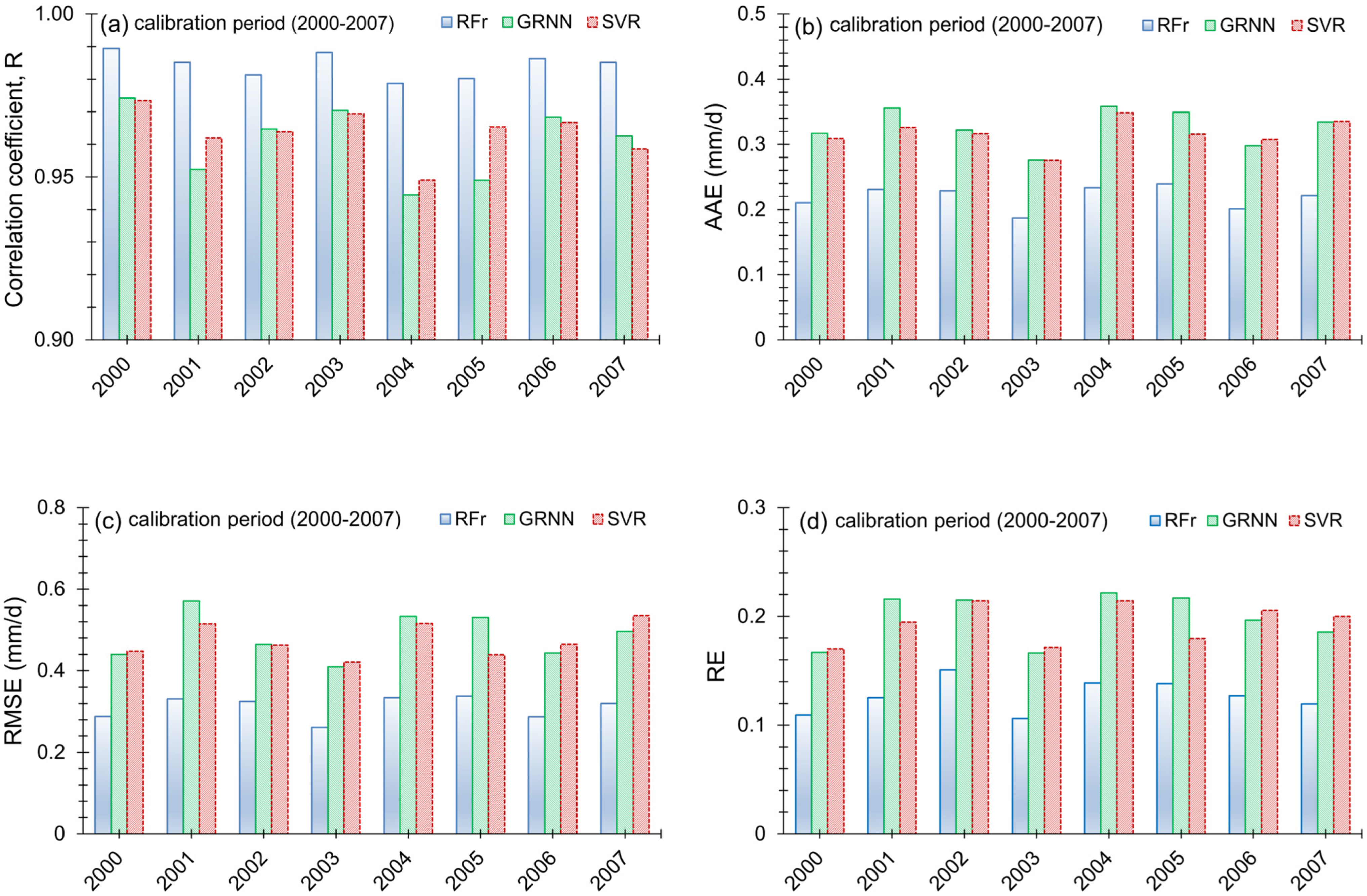
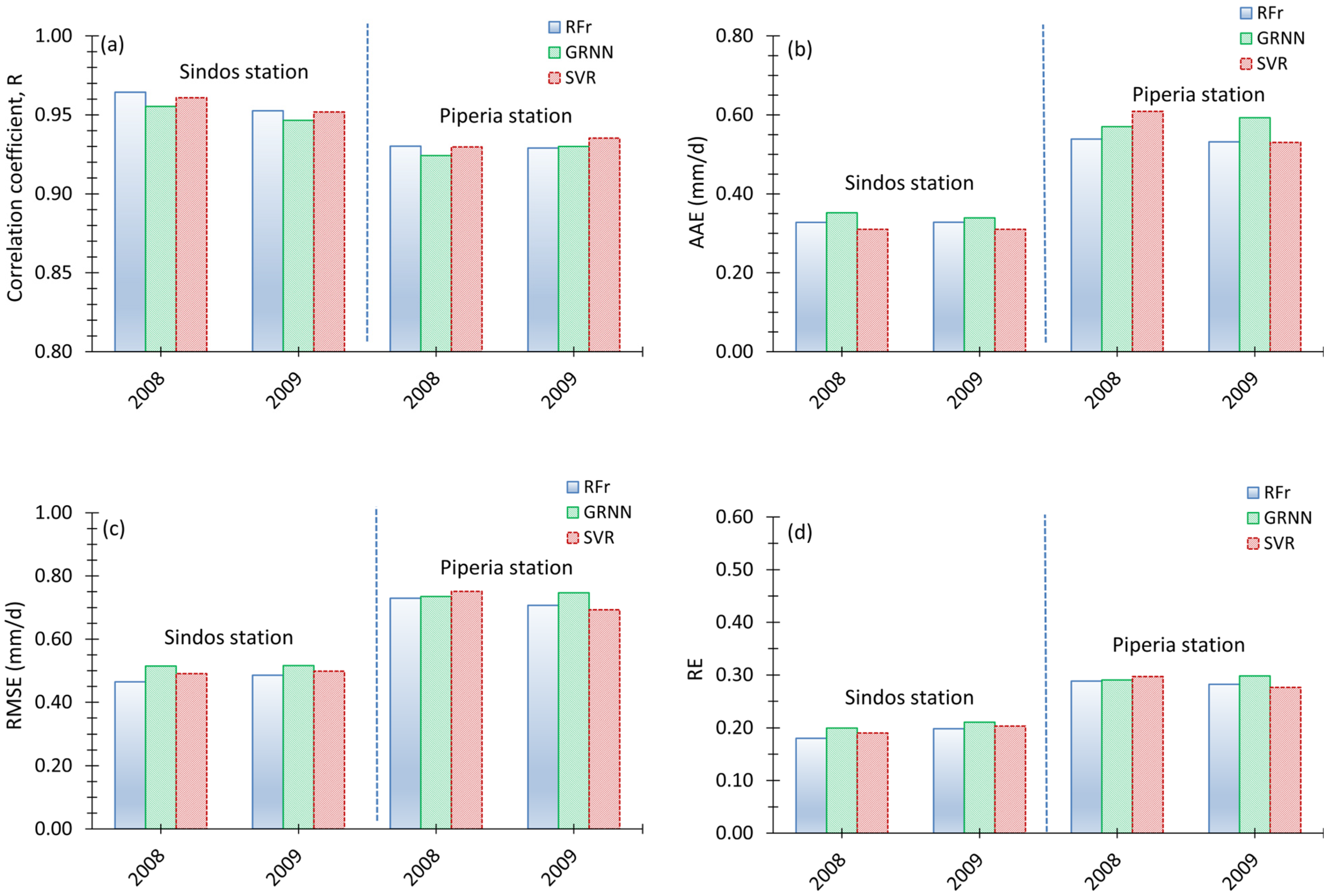
Performance of the Constructed Machine Learning Models

As non-parametric modeling approaches, machine learning methodologies do not impose assumptions. However, there are specific hyperparameters unique to each machine learning algorithm that need to be tuned to generate accurate and reliable models. In order for the best fitted RFr to be constructed, the optimal values of the training elements of the model were assessed through trial-and-error methodologies, taking into account the estimation and prediction mean square errors. Moreover, in order to guarantee full randomization of the procedure, the bootstrap aggregation technique was employed in the selection of training data for each individual decision tree during model building. To achieve this, 300 regression trees were utilized, each having 10 branches. These specific numbers were chosen after testing various options, ranging from 2 to 500 for the number of trees and 1 to 15 for the number of branches per tree. It was observed that once a combination of 300 regression trees with 10 branches each was employed, there was no substantial improvement in the model’s average estimation error. Additionally, this choice of tree depth effectively prevented the over-parameterization of the system during the learning process of the random forest regression (RFr) model.

Based on the models developed using generalized regression neural networks (GRNNs), the smoothing factor value (σ) was fine-tuned through an exhaustive grid-search approach [58], involving a total of 4950 fits. The optimal σ value, which resulted in the most precise and reliable model, was determined to be 1.489. An exhaustive grid-search approach was conducted to identify the best hyperparameter combination (ε, γ, and C) for constructing the ε-SVR model as well. The optimal hyperparameter values which resulted in both the highest correlation value and the smallest root mean square error between the observed and estimated ET_o values were determined to be 0.01, 0.5, and 180, respectively.

In

Table 1. Evaluation metrics for the estimated daily ET_o by the trained RFr, GRNN, and SVR models at Sindos station during the calibration period (2000–2007); n = 2922.

Evaluation Metrics	Machine Learning Models
	RFr	GRNN	SVR
R	0.9924	0.9576	0.9598
AAE	0.2189	0.3263	0.3168
RMSE	0.3119	0.4886	0.4766
RE%	12.67	19.86	19.36

, the evaluation metrics of the trained RFr, GRNN, and SVR models at Sindos station during the calibration period (2000–2007), using 2922 daily data points, are given. When evaluating the performance of the machine learning models constructed for the calibration dataset (Table 1), the RFr model demonstrated the most favorable fit to the data, achieving the highest R value and simultaneously the lowest values across all error metrics. The SVR model exhibited the second-best fit to the data, while the constructed GRNN model displayed comparatively lower adaptability, resulting in 1.49 times, 1.57 times, and 6.7% higher AAE, RMSE, and RE% values, respectively, compared to the error values obtained from the RFr model.

To assess the generalization capability of the created machine learning models, we computed evaluation metrics for a new time period spanning from 2008 to 2009, encompassing both the Sindos and Piperia stations. This analysis utilized 731 distinct daily input datasets for each station, and the outcomes can be found in

Table 2. Evaluation metrics for the predicted daily ET_o by the RFr, GRNN, and SVR models during the 2008–2009 period, for both Sindos and Piperia stations; n = 731.

Model	Sindos				Piperia
	R	AAE	RMSE	RE%	R	AAE	RMSE	RE%
RFr	0.9577	0.3278	0.4754	18.9	0.9368	0.4848	0.6376	25.3
GRNN	0.9491	0.3455	0.5156	20.5	0.9263	0.5814	0.7410	29.4
SVR	0.9548	0.3101	0.4944	19.7	0.9322	0.5697	0.7226	28.7

.

Table 2 illustrates that all the developed models exhibited effective generalization to new data, as evidenced by evaluation metric values closely resembling those obtained during the calibration period (Table 1). This indicates that the models delivered accurate ET_o predictions for new data, whether in the same station (Sindos) as the calibration data or in an entirely different station (Piperia). Furthermore, a consistent pattern in the evaluation metrics was observed among the models, with the RFr model generating the most precise predictions, followed by the SVR model, and the GRNN model producing the least accurate predictions.

To investigate the accuracy of estimation and prediction by the models on an annual basis, Figure 4 and Figure 5 were generated for each individual year.

The sub-figures in Figure 4 illustrate the performance of the RFr, GRNN, and SVR models at Sindos station, during the calibration period (2000–2007), for each individual year. It is important to highlight that these models were constructed using solely air temperature, Ra, and N data. In the case of Sindos station, shown in Figure 4, the performance metrics exhibited noticeable variability throughout the calibration period. Specifically, considering the RFr model, the values of R (Figure 4a) ranged from 0.9894 to 0.9851, with an average of 0.9843. The AAE values (Figure 4b) ranged from 0.2104 to 0.2211, averaging 0.2189 mm/d for the same model, while the RMSE values (Figure 4c) ranged from 0.2881 to 0.3201, with an average of 0.3108 mm/d. Lastly, the RE values (Figure 4d) ranged from 0.1093 to 0.1197, with an average value of 0.1269 for the best-performing RFr model. The GRNN and SVR models exhibited lower average R values, with their performance resulting in 2.39% and 2.11% lower average R values, respectively, compared to the average R value derived by the RFr model (Figure 4a). The SVR model yielded an average AAE value that was 1.45 times higher than that of the RFr model, while the GRNN model had an average AAE value 1.49 times higher than that of the RFr model. Additionally, the SVR model resulted in an average RMSE value that was 1.53 times smaller, and the GRNN model had an average RMSE value 1.56 times smaller than that of the RFr model.

Finally, the relative error (RE) in percentage error values for the GRNN and SVR models were 7.11% and 6.67% larger, respectively, compared to the average RE% value of the RFr model. The results mentioned above and shown in Figure 4 indicate that the constructed RFr model demonstrated the most effective fit with the calibration dataset.

Based on the evaluation of the machine learning models’ generalization capability using test datasets from Sindos and Piperia stations in the 2008–2009 testing period (Figure 5), the performance metrics for all models exhibited minor fluctuations, suggesting that the tested models possessed similar generalization abilities.

Figure 6 illustrates that there is minimal variability in annual ET_o values (mm/year) between the RFr, GRNN, SVR models, as well as the FAO 56 PM model, for the years 2000–2009 at Sindos station, as well as for the years 2008–2009 at Piperia station. When comparing these models to the reference FAO 56 PM ET_o values, at Sindos station, they tend to overestimate ET_o in 2002 and 2006 and underestimate ET_o in 2000, 2001, 2007, and 2008, with the RFr model performing better. Meanwhile, at Piperia station, the RFr model overestimated ET_o in 2008 and 2009, while the SVR model underestimated ET_o in the same years, with the GRNN model showing superior results.

According to [30,31], the Hargreaves–Samani (HG-S) method, which also relies on temperature data, has been effectively used in certain locations to estimate daily ET_o, and it is summarized by the following equation:

$${ET}_o={[0.0023 (T_{\mathit{mean}}+17.8\left)\right(T_{\mathit{max}}-T_{\mathit{min}}\left)\right]}^{0.5} R_{\alpha }$$

(11)

where ΕΤ_ο is the reference evapotranspiration (mm d⁻¹), T_mean is the mean daily air temperature (°C), T_max is the maximum daily air temperature (°C), T_min is the minimum daily air temperature (°C), and R_α is extraterrestrial radiation (mm d⁻¹), which can easily be estimated for a certain day and location using Equation (2).

Figure 7 displays the annual ET_o values (mm/year) estimated using the HG-S method at Sindos station for the period 2000–2009 and at Piperia station for the testing period 2008–2009. Figure 7 highlights a significant divergence between the annual ET_o values (mm/year) estimated using the FAO 56 PM and HG-S methods. At Sindos station, when comparing the HG-S method to the reference FAO 56 PM annual ET_o values, the HG-S method significantly overestimates ET_o for all years. The overestimation of annual ET_o values ranged from 20.29% to 41.20%, with an average of 29.33%. Conversely, at Piperia station, the HG-S method significantly underestimates the annual ET_o, with underestimation values of 48.61% for 2008 and 50.27% for 2009. Similar discrepancies are observed in the monthly ET_o values (mm/day) estimated by the two methods, confirming that the HG-S method has failed to reliably estimate daily ET_o at both stations.

Figure 8 demonstrates that there is minimal fluctuation in monthly ET_o values (mm/day) between the RFr, GRNN, SVR, and FAO 56 PM models. This consistency is observed during the calibration period from 2000 to 2007 at Sindos station (Figure 8a), as well as during the testing period, from 2008 to 2009, at both Sindos (Figure 8b) and Piperia (Figure 8c) stations. Notably, the RFr model consistently outperforms the other models in both periods.

Figure 9a,c,e depict scatterplots comparing ET_o values (mm/day) estimated by the FAO 56 PM model with those from the RFr, GRNN, and SVR models during the calibration period (2000–2007) at Sindos station. In these plots, it is obvious that the RFr model outperformed the GRNN and SVR models based on the slope of the fitted line equations and R² values (slope: 1.019 vs. 1.0073 and 0.9745; R²: 0.9662 vs. 0.9162 and 0.9212, respectively).

On the other hand, Figure 9b,d,f present scatterplots comparing ET_o values (mm/day) estimated by the FAO 56 PM model with those from the RFr, GRNN, and SVR models during the testing period (2008–2009) at Sindos station. Similar to the calibration period, the RFr model demonstrated superior performance compared to the GRNN and SVR models, as indicated by the slope of the fitted line equations and R² values (slope: 0.9875 vs. 0.9872 and 0.9596; R²: 0.9172 vs. 0.9022 and 0.91, respectively).

Figure 10a–c illustrate scatterplots that compare ET_o values (mm/day) estimated by the FAO 56 PM model with those from the RFr, GRNN, and SVR models during the testing period (2008–2009) at Piperia station. As can be seen (Figure 10), the RFr model has the highest R² value (0.8775), suggesting it explains the most variance in the data. However, its slope (0.8475) deviates significantly from 1, indicating it tends to underestimate the actual values. GRNN model has a lower R² value (0.8581) compared to the RFr model but has the slope (1.0035) closest to 1 and the intercept (0.0783) closest to 0, suggesting very accurate predictions, although it could not be able to explain the most variance in the data. Finally, SVR model showed a middle R² value (0.869), a slope (1.0114) close to 1, and a slightly higher intercept (0.1716) compared to the GRNN model. Although the results do not clearly identify the best prediction model for the Piperia test dataset, the overall performance of the RFr model on both the calibration and test datasets, compared to the GRNN and SVR models, suggests that the RFr model can be considered the safest choice.

4. Discussion

This study aims to offer a comprehensive and dependable methodology for estimating and predicting daily reference evapotranspiration (ET_o), which is of great importance for water resources management, water balance estimation, irrigation scheduling, agricultural production forecasting, and solving many theoretical problems in the fields of hydrology and meteorology. Given the nonlinear nature of ET_o, our approach involves employing three non-parametric regression-based machine learning modeling methods. This strategy is designed to leverage the unique strengths of each algorithm, while also taking into account their individual advantages and limitations.

The models were primarily constructed based on temperature data (Tmin, Tmax, Tmean), which are correlated. The effect of multicollinearity introduced in these non-parametric machine learning models can be considered minimal. Examining each modeling method used, it can be said that the ε-SVR approach effectively addresses the non-linear nature of the data by using kernel tricks to map input features to high-dimensional spaces, thus reducing issues from multicollinearity. Random forest (RFr) generally handles multicollinearity well. In our case, the model, composed of 300 regression trees with 10 branches each, was of moderate complexity. This tree depth effectively prevents over-parameterization during learning. Finally, generalized regression neural networks (GRNNs) are also less sensitive to multicollinearity due to their kernel regression principles. GRNNs, being inherently non-linear, do not assume linearity and base their predictions on the distance between input and training vectors, minimizing the impact of multicollinearity in high-dimensional spaces.

Additionally, all modeling approaches possess the capability to address data challenges like high variance, outliers, and potential missing values, ultimately resulting in accurate results. Nevertheless, it is essential to appropriately fine-tune the hyperparameters for all modeling approaches, as this task plays a crucial role in ensuring their effective estimation and prediction performance.

Specifically, the first utilized approach for ET_o estimation and prediction involves random forest regression (RFr), which, through the independent building of its decision trees, can effectively address the significant issue of overfitting while reducing the variance [60] and bias of predictions [61]. Nonetheless, it also exhibits a significant limitation, namely the absence of extrapolation capability. In other words, any forecast made outside the range of values encountered during the system’s construction phase will essentially be an average of the previously observed values within the RFr model’s scope. The further the predicted value is from the range of the training data, the less reliable the prediction becomes. The second modeling approach utilizes a generalized regression neural network (GRNN), which is a probabilistic neural network. It provides notable advantages [44], particularly in its ability to effectively converge towards the underlying data function, even in scenarios with a limited number of training samples. Furthermore, it requires minimal additional knowledge to achieve a satisfactory fit, eliminating the need for additional user input. As a result, the GRNN proves to be a valuable tool for making predictions and facilitating practical comparisons of system performance. However, due to the fact that it is a memory-intensive neural network, GRNN cannot be considered as a suitable neural network type for large datasets or high-dimensional data. Furthermore, it can be prone to overfitting, which is a common problem for all neural network types. Due to ε-SVR’s ability to uncover intricate relationships within real-world data and effectively address issues like overfitting and local minima [61,62], the support vector regression approach was our third viable choice for estimating and predicting ET_o. However, training an SVR model is a computationally intensive procedure.

Taking into account the flexibility exhibited by each of the employed approaches, as shown in Table 1, and their capacity to generalize to new datasets, as indicated in Table 2, it is reasonable to deem their performance as satisfactory for both calibration and the two distinct test datasets. Additionally, there was consistency observed in how they performed in terms of estimation and prediction accuracy.

The modeling of daily ET_o by the developed RFr, GRNN, and SVR models, using only temperature data, offers the possibility of integrating ET_o in many cases, under current and climate change conditions, when temperature data are available. Some of its uses include the prediction of the agricultural production through the reliable estimation of the crop water requirements and its introduction in each grid of distributed hydrological models for the accurate estimation of the water balance components.

At this point, it is noteworthy to say that the Hargreaves–Samani (HG-S) method [30,31], which also assess temperature-based features for estimation ET_o, was examined in this paper, and the finding is that it has failed at reliable daily ET_o estimation at both stations.

5. Conclusions

This study delved into the feasibility of utilizing three different regression-based machine learning models to estimate daily reference evapotranspiration (ET_o): random forest regression (RFr), generalized regression neural networks (GRNNs), and support vector regression (SVR).We employed meteorological data from two stations situated in northern Greece, focusing solely on temperature variables (T_min, T_max, T_mean), extraterrestrial radiation (R_a), and theoretical sunshine (N) as input parameters for the models. To assess performance, we compared the results with FAO 56 PM daily ET_o values estimated using comprehensive meteorological data, which served as our reference benchmark.

Analyzing the statistical comparisons (both numerically and graphically), encompassing evaluation metrics like R, AAE, RMSE, and RE%, alongside a comprehensive examination of the models’ performance throughout the entire calibration and testing periods, as well as on a yearly basis, it becomes obvious that all three models (RFr, GRNN, and SVR) consistently displayed robust performance when estimating daily ET_o at both stations. Notably, the RFr model stood out as the top performer, providing the most precise daily ET_o estimates.

This study’s findings suggest the utilization of three regression-based machine learning models (RFr, GRNN, and SVR) as valuable tools for estimating daily ET_o with only temperature data. Once these regression-based machine learning models have been successfully developed, they have the potential to serve as effective alternatives for estimating daily ET_o, under current and climate change conditions, when temperature data are available.

Daily ET_o is crucial information for water resources management and particularly for the prediction of agricultural production under climate change conditions. Machine learning models offer several advantages, including their ability to support engineers and watershed managers in diverse applications. As the models run on a daily time step, selecting two stations in different regions with significantly different altitudes (10 m and 160 m) ensures the integration of diverse meteorological variable values.

It is worth noting that this study utilized data from two stations, and future research could explore the application of the RFr, GRNN, and SVR models with data from additional stations. Additionally, the significant limitation of the RFr model—its lack of extrapolation capability—must be seriously considered, as it could impact its prediction accuracy.

Finally, it would be interesting for future research to include a comparison of these approaches, which have demonstrated potential in accurately estimating and predicting ET_o, against more complex machine learning models to further evaluate their relative performance.

References

1. Jamshidi, S.; Zand-parsa, S.; Pakparvar, M.; Niyogi, D. Evaluation of Evapotranspiration over a Semiarid Region Using Multiresolution Data Sources. J. Hydrometeorol. 2019, 20, 947–964. [Google Scholar] [CrossRef]
2. Bellido-Jiménez, J.A.; Estévez, J.; García-Marín, A.P. New machine learning approaches to improve reference evapotranspiration estimates using intra-daily temperature-based variables in a semi-arid region of Spain. Agric. Water Manag. 2021, 245, 106558. [Google Scholar] [CrossRef]
3. Dimitriadou, S.; Nikolakopoulos, K.G. Evapotranspiration Trends and Interactions in Light of the Anthropogenic Footprint and the Climate Crisis: A Review. Hydrology 2021, 8, 163. [Google Scholar] [CrossRef]
4. Zare, M.; Pakparvar, M.; Jamshidi, S.; Bazrafshan, O.; Ghabari, G. Optimizing the Runoff Estimation with HEC-HMS Model Using Spatial Evapotranspiration by the SEBS Model. Water Resour. Manag. 2021, 35, 2633–2648. [Google Scholar] [CrossRef]
5. Jamshidi, S.; Zand-Parsa, S.; Kamgar-Haghighi, A.A.; Shahsavar, A.R.; Niyogi, D. Evapotranspiration, crop coefficients, and physiological responses of citrus trees in semi-arid climatic conditions. Agric. Water Manag. 2020, 227, 105838. [Google Scholar] [CrossRef]
6. Niyogi, D.; Jamshidi, S.; Smith, D.; Kellner, O. Evapotranspiration Climatology of Indiana Using In Situ and Remotely Sensed Products. J. Appl. Meteorol. Climatol. 2020, 59, 2093–2111. [Google Scholar] [CrossRef]
7. Malamos, N.; Tegos, A. Advances in Evaporation and Evaporative Demand. Hydrology 2022, 9, 78. [Google Scholar] [CrossRef]
8. ASCE-EWRI. Task Committee on Standardization of Reference Evapotranspiration, Principal; Report 0-7844-0805-X. The ASCE Standardized Reference Evapotranspiration Equation; Allen, R.G., Walter, I.A., Elliott, R.L., Howell, T.A., Itenfisu, D., Jensen, M.E., Snyder, R.L., Eds.; American Society of Civil Engineers (ASCE): Reston, VA, USA, 2005. [Google Scholar]
9. Allen, R.G.; Pereira, L.S.; Raes, D.; Smith, M. Crop evapotranspiration-Guidelines for computing crop water requirements. In Irrigation and Drainage; Paper No. 56; FAO: Rome, Italy, 1998; Volume 300. [Google Scholar]
10. ASCE Task Committee on Application of Artificial Neural Networks in Hydrology. Artificial neural networks in Hydrology. I. Preliminary concepts. J. Hydrol. Eng. 2000, 5, 115–123. [Google Scholar] [CrossRef]
11. Agarwal, J.; Singh, R.D. Runoff modeling through back propagation artificial neural networks with variable rainfall-runoff data. Water Resour. Manag. 2004, 18, 285–300. [Google Scholar] [CrossRef]
12. Diamantopoulou, M.J.; Antonopoulos, V.; Papamichail, D. Cascade correlation artificial neural networks for estimating missing monthly values of water quality parameters in rivers. Water Resour. Manag. 2007, 21, 649–662. [Google Scholar] [CrossRef]
13. Diamantopoulou, M.J.; Georgiou, P.; Papamichail, D. Performance of neural network models with Kalman learning rule for flow routing in a river system. Fresen. Environ. Bull. 2007, 16, 1474–1484. [Google Scholar]
14. Gupta, R.; Singh, A.N.; Singhal, A. Application of ANN for water quality index. Int. J. Mach. Learn. Comput. 2019, 9, 688–693. [Google Scholar] [CrossRef]
15. Abba, S.I.; Pham, Q.B.; Saini, G.; Linh, N.T.T.; Ahmed, A.N.; Mohajane, M.; Khaledian, M.; Abdulkadir, R.A.; Bach, Q.V. Implementation of data intelligence models coupled with ensemble machine learning for prediction of water quality index. Environ. Sci. Pollut. Res. 2020, 27, 41524–41539. [Google Scholar] [CrossRef]
16. Jennifer, J.J. Feature elimination and comparison of machine learning algorithms in landslide susceptibility mapping. Environ. Earth Sci. 2022, 81, 489. [Google Scholar] [CrossRef]
17. Ishfaque, M.; Dai, Q.; Wahid, A.; Saddique, B.; Jadoon, K.Z.; Janjuhah, H.T.; Shahzad, S.M. Trend analysis of hydro-climatological parameters and assessment of climate impact on dam seepage using statistical and machine learning models. Environ. Earth Sci. 2023, 82, 1–22. [Google Scholar] [CrossRef]
18. Diamantopoulou, M.J.; Georgiou, P.; Papamichail, D. Performance evaluation of artificial neural networks in estimating reference evapotranspiration with minimal meteorological data. Glob. Nest 2011, 13, 18–27. [Google Scholar]
19. Ladlani, I.; Houichi, L.; Djemili, L.; Heddam, S.; Belouz, K. Modeling daily reference evapotranspiration (ETo) in the north of Algeria using generalized regression neural networks (GRNN) and radial basis function neural networks (RBFNN): A comparative study. Meteorol. Atmos. Phys. 2012, 118, 163–178. [Google Scholar] [CrossRef]
20. Kişi, O. Modeling reference evapotranspiration using three different heuristic regression approaches. Agric. Water Manag. 2016, 169, 162–172. [Google Scholar] [CrossRef]
21. Antonopoulos, V.Z.; Antonopoulos, A.Z. Daily reference evapotranspiration estimates by artificial neural networks techniques and empirical equations using limited input variables. Comput. Electron. Agric. 2017, 132, 86–96. [Google Scholar] [CrossRef]
22. Feng, Y.; Cui, N.; Gong, D.; Zhang, Q.; Zhao, L. Evaluation of random forests and generalized regression neural networks for daily reference evapotranspiration modeling. Agric. Water Manag. 2017, 193, 163–173. [Google Scholar] [CrossRef]
23. Mehdizadeh, S.; Mohammadi, B.; Pham, Q.B.; Duan, Z. Development of boosted machine learning models for estimating daily reference evapotranspiration and comparison with empirical approaches. Water 2021, 13, 3489. [Google Scholar] [CrossRef]
24. Rashid Niaghi, A.; Hassanijalilian, O.; Shiri, J. Estimation of reference evapotranspiration using spatial and temporal machine learning approaches. Hydrology 2021, 8, 25. [Google Scholar] [CrossRef]
25. Kim, S.J.; Bae, S.J.; Jang, M.W. Linear regression machine learning algorithms for estimating reference evapotranspiration using limited climate data. Sustainability 2022, 14, 11674. [Google Scholar] [CrossRef]
26. Tejada, A.T.J.; Ella, V.B.; Lampayan, R.M.; Reano, C.E. Modeling reference crop evapotranspiration using support vector machine (SVM) and extreme learning machine (ELM) in region IV-A. Philipp. Water 2022, 14, 754. [Google Scholar] [CrossRef]
27. Zouzou, Y.; Citakoglu, H. General and regional cross-station assessment of machine learning models for estimating reference evapotranspiration. Acta Geophys. 2023, 71, 927–947. [Google Scholar] [CrossRef]
28. Raza, A.; Fahmeed, R.; Syed, N.R.; Katipoglu, O.M.; Zubair, M.; Alshehri, F.; Elbeltagi, A. Performance Evaluation of Five Machine Learning Algorithms for Estimating Reference Evapotranspiration in an Arid Climate. Water 2023, 15, 3822. [Google Scholar] [CrossRef]
29. Yildirim, D.; Kόηόktopcu, E.; Cemek, B.; Simsek, H. Comparison of machine learning techniques and spatial distribution of daily reference evapotranspiration in Turkiye. Appl. Water Sci. 2023, 13, 107. [Google Scholar] [CrossRef]
30. Hargreaves, G.H. and Samani, Z.A. Reference crop evapotranspiration from temperature. Appl. Eng. Agric. 1985, 1, 96–99. [Google Scholar] [CrossRef]
31. Hargreaves, G.H. and Allen, R.G. History and evaluation of Hargreaves evapotranspiration equation. J. Irrig. Drain. Eng. 2003, 129, 53–63. [Google Scholar] [CrossRef]
32. Russell, S.; Norvig, P. Artificial Intelligence: A Modern Approach (Pearson Series in Artificial Intelligence), 4th ed.; Pearson: London, UK, 2020; p. 1136. [Google Scholar]
33. Bates, D.; Watts, D.G. Nonlinear Regression Analysis and Its Applications; Wiley Series in Probability and Statistics; Wiley: New York, NY, USA, 1988. [Google Scholar]
34. Biau, G.; Scornet, E. A random forest guided tour. Test 2006, 25, 197–227. [Google Scholar] [CrossRef]
35. Breiman, L. Random Forests. Mach. Learn. 2001, 45, 5–32. [Google Scholar] [CrossRef]
36. Breiman, L. Some Infinity Theory for Predictor Ensembles; Technical Report 579, Statistics Dept. UCB: Berkeley, CA, USA, 2000. [Google Scholar]
37. Breskvar, M.; Kocev, D.; Džeroski, S. Ensembles for multi-target regression with random output selections. Mach. Learn. 2018, 107, 1673–1709. [Google Scholar] [CrossRef]
38. Shahhosseini, M.; Hu, G.; Pham, H. Optimizing ensemble weights and hyperparameters of machine learning models for regression problems. Mach. Learn. Appl. 2022, 7, 100251. [Google Scholar] [CrossRef]
39. Breiman, L. Bagging predictors. Mach. Learn. 1996, 26, 123–140. [Google Scholar] [CrossRef]
40. Segal, M.R. Machine Learning Benchmarks and Random Forest Regression; Center for Bioinformatics and Molecular Biostatistics, University of California: Sun Francisco, CA, USA, 2003; Available online: https://escholarship.org/uc/item/35x3v9t4 (accessed on 10 June 2024).
41. Prasad, A.M.; Iverson, L.; Liaw, A. Newer Classification and Regression Techniques: Bagging and Random Forests for Ecological Prediction. Ecosystems 2006, 9, 181–199. [Google Scholar] [CrossRef]
42. Hastie, T.; Tibshirani, R.; Tibshirani, R.J. Extended Comparisons of Best Subset Selection, Forward Stepwise Selection, and the lasso. arXiv 2017, arXiv:1707.08692. Available online: http://jmlr.org/papers/v12/pedregosa11a.html (accessed on 10 June 2024).
43. Diamantopoulou, M.J. Simulation of over-bark tree bole diameters, through the RFr (Random Forest Regression) algorithm. Folia Oecologica 2022, 49, 93–101. [Google Scholar] [CrossRef]
44. Specht, D.F. A general regression neural network. IEEE Trans. Neural Netw. 1991, 2, 568–576. [Google Scholar] [CrossRef]
45. Kim, S.; Kim, H.S. Neural networks and genetic algorithm approach for nonlinear evaporation and evapotranspiration modeling. J. Hydrol. 2008, 351, 299–317. [Google Scholar] [CrossRef]
46. Kumar, M.; Raghuwanshi, N.S.; Singh, R. Artificial neural networks approach in evapotranspiration modeling: A review. Irrig. Sci. 2011, 29, 11–25. [Google Scholar] [CrossRef]
47. Dreyfus, G. Neural Networks: Methodology and Applications; Springer Science & Business Media: Berlin, Germany, 2005. [Google Scholar]
48. Cigizoglu, H.K.; Alp, M. Generalized regression neural network in modeling river sediment yield. Adv. Eng. Softw. 2006, 37, 63–68. [Google Scholar] [CrossRef]
49. de Bragança Pereira, B.; Rao, C.R.; de Oliveira, F.B. Statistical Learning Using Neural Networks: A Guide for Statisticians and Data Scientists with Python; CRC Press: Boca Raton, FL, USA, 2020. [Google Scholar]
50. Belete, D.M.; Huchaiah, M.D. Grid search in hyperparameter optimization of machine learning models for prediction of HIV/AIDS test results. Int. J. Comput. Appl. 2022, 44, 875–886. [Google Scholar] [CrossRef]
51. Vapnik, V.N. Three fundamental concepts of the capacity of learning machines. Phys. A Stat. Mech. Its Appl. 1993, 200, 538–544. [Google Scholar] [CrossRef]
52. Cortes, C.; Vapnik, V.N. Support Vector Networks. Mach. Learn. 1995, 20, 273–297. [Google Scholar] [CrossRef]
53. Vapnik, V.N. An Overview of Statistical Learning Theory. IEEE Trans. Neural Netw. 1999, 10, 988–999. [Google Scholar] [CrossRef]
54. Vapnik, V.N. The Nature of Statistical Learning Theory, 2nd ed.; Springer: Berlin, Germany, 2000. [Google Scholar] [CrossRef]
55. Vapnik, V.N.; Golowich, S.; Smola, A. Support Vector Method for Function Approximation, Regression Estimation, and Signal Processing. In Advances in Neural Information Processing Systems 9; MIT Press: Cambridge, MA, USA, 1997. [Google Scholar]
56. Smola, A.J.; Schölkopf, B. On a kernel-based method for pattern recognition, regression, approximation, and operator inversion. Algorithmica 1998, 22, 211–231. [Google Scholar] [CrossRef]
57. Cristianini, N.; Shawe-Taylor, J. An Introduction to Support Vector Machines and Other Kernel-Based Learning Methods; Cambridge University Press: Cambridge, UK, 2000; p. 189. [Google Scholar]
58. Pedregosa, F.; Varoquaux, G.; Gramfort, A.; Michel, V.; Thirion, B.; Grisel, O.; Blondel, M.; Prettenhofer, P.; Weiss, R.; Dubourg, V.; et al.; et al. Scikit-learn: Machine Learning in Python. J. Mach. Learn. Res. 2011, 12, 2825–2830. [Google Scholar] [CrossRef]
59. Python Software Foundation. © Copyright 2001–2022. 2022. Available online: https://docs.python.org/3.9/index.html (accessed on 20 June 2024).
60. Genuer, R. Variance reduction in purely random forests. J. Nonparametric Stat. 2012, 24, 543–562. [Google Scholar] [CrossRef]
61. Diamantopoulou, M.J.; Özçelik, R.; Yavuz, H. Tree-bark volume prediction via machine learning: A case study based on black alder’s tree-bark production. Comput. Electron. Agric. 2018, 151, 431–440. [Google Scholar] [CrossRef]
62. Wang, L.; Niu, Z.; Kisi, O.; Li, C.; Yu, D. Pan evaporation modeling using four different heuristic approaches. Com. Elec. Agric. 2017, 140, 203–213. [Google Scholar] [CrossRef]
Figure 1. Geographic location of the meteorological stations in Greece.
Hydrology 11 00089 g001
Figure 2. Monthly variation in meteorological variables and ETo at Sindos station, during the training (2000–2007) and test (2008–2009) period, and at Piperia station, during the test (2008–2009) period (ae). Tmean, RH, U2, Rn, and ETo represent mean air temperature, relative humidity, wind speed, net solar radiation, and reference evapotranspiration estimated by the FAO 56 PM method, respectively.
Hydrology 11 00089 g002
Figure 3. Inter-annual variation in meteorological variables and ETo at Sindos station during 2000–2009 (a1,b1,c1,d1,e1) and at Piperia station during 2008–2009 (a2,b2,c2,d2,e2). Tmean, RH, U2, Rn, and ETo represent mean air temperature, relative humidity, wind speed, net solar radiation, and reference evapotranspiration estimated by the FAO 56 PM method, respectively.
Hydrology 11 00089 g003aHydrology 11 00089 g003b
Figure 4. Performance of RFr, GRNN, and SVR models at Sindos station, during calibration (2000–2007) period. R (a), AAE (b), RMSE (c), and RE (d) represent correlation coefficient, absolute average error, root mean square error, and relative error, respectively.
Hydrology 11 00089 g004
Figure 5. Performance of RFr, GRNN, and SVR models at Sindos and Piperia stations during testing (2008–2009) period. R (a), AAE (b), RMSE (c), and RE (d) represent correlation coefficient, absolute average error, root mean square error, and relative error, respectively.
Hydrology 11 00089 g005
Figure 6. Annual variations in ETo values (mm/year) estimated by FAO 56 PM and RFr, GRNN, and SVR models at (a) Sindos station during (2000–2009) period and (b) Piperia station during testing (2008–2009) period.
Hydrology 11 00089 g006
Figure 7. Annual variations in ETo values (mm/year) estimated by FAO 56 PM and HG-S models at (a) Sindos station during (2000–2009) period and (b) Piperia station during testing (2008–2009) period.
Hydrology 11 00089 g007
Figure 8. Monthly variations in ETo values (mm/d) estimated by FAO 56 PM and RFr, GRNN, and SVR models at (a) Sindos station during calibration (2000–2007) period, (b) Sindos station during testing (2008–2009) period, and (c) Piperia station during testing (2008–2009) period.
Hydrology 11 00089 g008
Figure 9. Scatterplots of ETo values (mm/d) estimated by FAO 56 PM and RFr, GRNN, and SVR models, during calibration (2000–2007) period (a,c,e) and during testing (2008–2009) period (b,d,f), respectively, at Sindos station.
Hydrology 11 00089 g009
Figure 10. Scatterplots of ETo values (mm/d) estimated by FAO 56 PM and RFr, GRNN, and SVR models, respectively, during testing (2008–2009) period (a,b,c) at Piperia station.
Hydrology 11 00089 g010