Article

A Modified Xinanjiang Model for Quantifying Streamflow Components in a Typical Watershed in Eastern China

by
Kaibin Wu
1,
Minpeng Hu
1,
Yu Zhang
1,
Jia Zhou
1 and
Dingjiang Chen
1,2,3,*
1
College of Environmental & Resource Sciences, Zhejiang University, Hangzhou 310058, China
2
Ministry of Education Key Laboratory of Environment Remediation and Ecological Health, Zhejiang University, Hangzhou 310058, China
3
Zhejiang Provincial Key Laboratory of Agricultural Resources and Environment, Zhejiang University, Hangzhou 310058, China
*
Author to whom correspondence should be addressed.
Hydrology 2024, 11(7), 90; https://doi.org/10.3390/hydrology11070090
Submission received: 1 June 2024 / Revised: 21 June 2024 / Accepted: 22 June 2024 / Published: 25 June 2024

Abstract

:
An accurate quantification of flow components and an understanding of water source dynamics are essential for effective water resource and quality management. However, the complexity of hydrological processes and the interference of intensive human activities pose significant challenges in precisely separating water discharge into distinct components such as surface runoff, interflow, and groundwater. The Xinanjiang (XAJ) model, a conceptual watershed hydrological model, has been developed and successfully implemented for rainfall–runoff simulations and hydrograph separations across various Chinese watersheds. While the model framework is robust, it fails to account for agricultural irrigation water withdrawals and the variations in in-stream water travel times across different hydrological regimes, introducing considerable uncertainty in simulating low-flow conditions. This study introduced modifications to the XAJ model by allowing parameter adjustments across different flow regimes and incorporating irrigation withdrawals into the runoff routing process. Utilizing a decade of hydrometeorological data (2013–2022) from the Yongan River watershed in eastern China, the modified model demonstrated improved efficiency metrics in low- and medium-flow regimes compared to the original model, with a Nash–Sutcliffe coefficient improvement from −4.43~−0.49 to 0.40~0.46, R2 from 0.21~0.36 to 0.53~0.63, and BIAS reduction from 7.60~89.08% to 2.06~12.71%. Furthermore, the modified XAJ model provided a more accurate estimation of the spatial and temporal distribution of streamflow components across sub-watersheds. The original model tended to overestimate groundwater contributions (13%) and underestimate interflow (14%), particularly in low-flow conditions. The enhanced XAJ model, thus, offers a more effective tool for identifying streamflow components, providing essential insights into hydrological processes for better management decisions.

1. Introduction

The quantitative understanding of water source dynamics is crucial for understanding the hydrological cycle [1,2], assessing water quantity and quality [3,4], protecting aquatic ecosystems and biodiversity [5], and scientifically managing water resources [6]. Various methods are available to quantify flow components, including graphical methods [7], digital filter techniques [8,9], recession curve analysis [10], and tracer-based separations using isotopes [2,11] and chemicals [12,13]. Additionally, watershed models have been increasingly used to study these dynamics [14,15,16].
The Xinanjiang model (XAJ), one of the most popular watershed models in China, serves as a crucial tool for rainfall–runoff simulation, hydrograph separation, and water resource management [16,17]. The fundamental hypothesis of the model is that runoff does not occur until the soil moisture in the aeration zone reaches field capacity. By separating streamflow into surface runoff, interflow, and groundwater, and incorporating the principles of hillslope hydrology and Horton infiltration, the XAJ model has significantly improved simulation accuracy. Since its development, it has been effectively applied in the humid and semi-humid regions of China for rainfall–runoff simulations [18]. When compared to other hydrological models (e.g., the NAM model, Sacramento model, SMAR model), the XAJ model demonstrates superior runoff simulation capabilities [19,20,21,22] and has been incorporated into the China National Flood Forecasting System [23]. Coupling with ArcGIS and remote sensing technology further improved the prediction and application of the XAJ model in ungauged catchments [24,25]. Furthermore, the use of the XAJ model has advanced our understanding of local hydrological processes and streamflow components. Increasing studies have explored rapid and slow subsurface flows in karst systems [16], the impact of small water structures on streamflow components [26], the proportion of streamflow components in karst areas [27], the factors influencing different streamflow contributions in humid hilly areas [28], and the separation of snowmelt and glacier melt runoff in cryosphere and snow-melting areas [29,30].
However, many studies utilizing the XAJ model have primarily focused on peak-flow simulations, often neglecting low-flow conditions that are crucial for water supply, water quality, and aquatic ecosystems [31,32,33]. Thus, the model has demonstrated lower accuracy and greater uncertainty in simulations under low-flow conditions [34]. For instance, in the Poyang Lake basin, median Nash–Sutcliffe Efficiency (NSE) values were 0.62 for high-flow and just 0.25 for low-flow conditions [35]. Similarly, in the Chaohu Lake, the accuracy for low-inflow years (NSE: 0.63) was worse compared to high/normal-inflow years (NSE: 0.82/0.72) [36]. Limitations such as fixed model parameters and model structure may hinder accurate discharge simulations under low-flow conditions. A significant shortcoming of the XAJ model is that it fails to adjust parameters to accommodate changes in stream channel water travel times between high- and low-flow conditions [34]. Streamflow discharge and velocity are positively correlated, leading to water travel times in the same stream channel lengths that can vary significantly from a few hours to several dozen hours under varying discharge conditions [37]. To overcome these shortcomings, physical mechanism-based models incorporating the kinematic wave model have been developed to account for variable travel times in channelized flow [38,39,40]. Furthermore, the original XAJ model was designed for natural watersheds and did not account for the impact of human activities on streamflow calculations. Therefore, the model’s lack of consideration for agricultural irrigation withdrawals, which can significantly reduce streamflow and alter its components [41,42], might be another reason for its inadequate low-flow simulations [43]. Although some studies have attempted to integrate agricultural irrigation modules into the XAJ model, there has not yet been an effective analysis of the impact of irrigation on streamflow discharge [44]. Several hydrological models that account for irrigation typically specify the timing, application amount, and source of irrigation, such as the enhanced VIC land surface model in the Mekong River Basin [45], the irrigation module of the SWAT model [40], and the WetSpa-WW model, which quantifies the impact of agricultural water consumption [46]. These models highlight the critical need to consider irrigation withdrawals and variable travel times in stream channel modeling.
This study aims to enhance streamflow discharge simulations under low-flow conditions using the XAJ model, particularly focusing on in-stream water travel time variations and agricultural irrigation withdrawals. We validated the accuracy of the improved model with a decade of hydrometeorological data (2013–2022) from the Yongan River watershed in eastern China, a typical region with significant agricultural irrigation demands. The primary objectives were to (i) adjust the XAJ model to account for daily agricultural irrigation water withdrawals and variable travel times in the stream channel, (ii) verify the model simulation results and assess the impacts of these modifications, and (iii) capture the spatiotemporal dynamics of streamflow components across the watershed. The modified model retains the original strengths but overcomes its previous limitations, thus offering a more precise tool for effective water resource management.

2. Materials and Methods
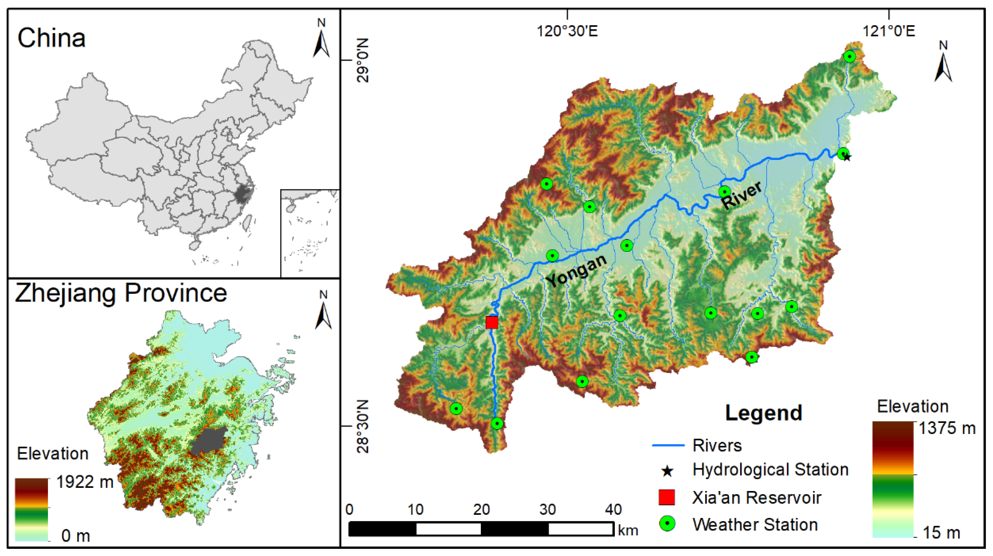
2.1. Study Area

The Yongan River watershed (120°13′46″–121°0′52″ E and 28°28′10″–29°2′22″ N; elevation of ~15–1000 m; mean slope gradient of 21.5°) is located in the highly developed Taizhou region of the Zhejiang Province in eastern China (Figure 1). The Yongan River is the third largest river in the Zhejiang Province and one of eight major river systems in the area, flowing into the Taizhou Estuary and the East China Sea. The hydrological station for this study (BZA, Figure 1) is situated 55 km upstream of the Taizhou Estuary at an elevation of ~15 m. The river encompasses a drainage area of 2474 km2, with an average annual water depth of 5.42 m, and a discharge rate of 72.9 m3 s−1 at the sampling point. The main stream (141 km long) does not experience transboundary water withdrawals, and there were no significant trends in annual precipitation or average river discharge throughout the study period.
The region has a subtropical monsoon climate, with an average annual precipitation of 1400 mm and an average temperature of 17.4 °C. Rainfall primarily occurs from May to September, coinciding with the typhoon season. Agricultural land, including paddy fields, garden plots, and dry land, accounted for 16.6% of the total watershed area during the study periods. Developed areas, which include rural and urban residential lands, roads, and mining/industrial lands, made up 1.4% of the area, while woodlands (broadleaf), barren lands, and water surfaces contributed 79.3%, 1.4%, and 1.3%, respectively. Red (Oxisols), yellow (Ultisols), and lithological (Entisols) soil groups accounted for 64.6%, 15.4%, and 1.5% of the total soil area, respectively. The main local crops are cereals (rice, wheat, and corn), beans, potatoes, cash crops, and orchard fruits. Due to the climatic conditions, agricultural activities in the watershed exhibit noticeable seasonal changes. The majority of agricultural activities occur from May to October (the growing season), while fewer activities take place from November to April (the dormant season).
Enhancing and advocating for water conservation and irrigation projects in farmland have consistently been pivotal endeavors in the watershed. The Xia’an Reservoir, a comprehensive large-scale hydraulic project, is located upstream of the Yongan River watershed (Figure 1) and serves as the sole controlling project within the watershed. Constructed in 2003, it has a total storage capacity of 135 million cubic meters and functions primarily for flood control, irrigation (water supply), and power generation. Since 2000, the area of agricultural land irrigated and drained using cement channels and pipes has approximately doubled, replacing the old irrigation and drainage systems constructed from stone and mud in the 1950s [47]. Data from yearbooks of neighboring counties and cities indicate that the effective irrigated area can cover approximately 90% of the total cultivated land area. The effective irrigated agricultural area in the watershed ranged from 16,000 to 17,800 hectares over the 2013–2022 period. During the study period, irrigation water consumption in the watershed ranged from 4320 to 5145 m3 ha−1 a year−1 (Figure 2). According to the third soil survey in the Zhejiang Province, the predominant irrigation method in this area involves open-channel water diversion, with 99% of agricultural irrigation water sourced from surface water.

2.2. Data Sources

Daily precipitation amounts at seventeen weather monitoring stations and daily pan evaporation amounts at three weather monitoring stations within the watershed for the 2013–2022 period were obtained from the local Hydrology Bureau and the Weather Bureau of Taizhou, respectively. Evapotranspiration was measured using the E601 pan evaporator in accordance with national specifications for surface meteorological observation (GB/T 35230-2017). Daily river discharge data at the watershed outlet (BZA) and daily outflows from upstream reservoirs (Xia’an Reservoir) were also collected from local authorities. Annual average agricultural irrigation withdrawal data and total irrigation water consumption were obtained from the Annual Water Resources Announcement of the Taizhou Water Resources Bureau. Agricultural information was derived from local government yearbooks of Xianju County and Linhai City. Remote sensing images and DEM data of the watershed were provided by Geospatial Data Cloud site, Computer Network Information Center, Chinese Academy of Sciences. The soil data were obtained from the Food and Agriculture Organization of the United Nations (FAO).

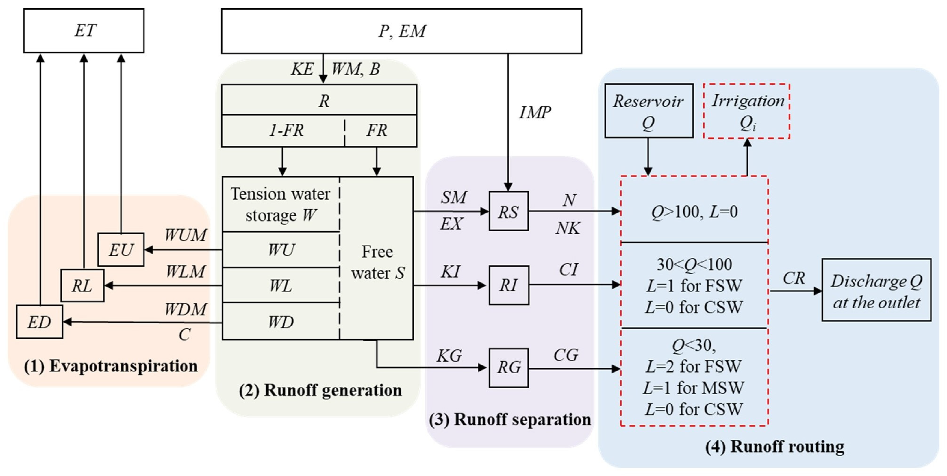
2.3. The Modification of the Xinanjiang Model

The Xinanjiang (XAJ) model is a conceptual rainfall–runoff model designed to simulate the hydrological processes in a watershed. It comprises four computational modules: an evapotranspiration module, a runoff generation module, a runoff separation module, and a runoff routing module (Figure 3). These modules collectively illustrate the general process of water movement from precipitation to streamflow [17]. In the runoff separation module, the free water reservoir structure is employed to divide the runoff into surface runoff, interflow, and groundwater. Due to its simple structure and the physical basis of the processes, the model has shown good performance in simulating runoff in the humid region of southern China [48]. A more detailed description of the model and its 15 parameters (Table 1) can be found in previous studies [49].
Different values of stream discharge in the same river channel correspond to varying river velocities, which in turn lead to variations in travel time [50,51]. To account for this, the runoff routing module in the modified XAJ model was revised to incorporate the lag stream channel routing approach with variable parameters:
Qt = CR × Qi,t−L + (1 − CR) × (QSi,t−L + QIi,t−L + QGi,t−L)
where L is the lag time, measured in days; CR is the recession constant; and QS, QI, and QG are the surface runoff, interflow, and groundwater outflow, respectively, and the unit of discharge is m3 s−1.
Based on the analysis of the observed precipitation and discharge data, the water travel time in the stream channel ranged from 0 to 2 days. The runoff routing module was divided into three regimes: (1) discharge above 100 m3 s−1 as a high-flow regime; (2) discharge between 30–100 m3 s−1 as a medium-flow regime; and (3) discharge below 30 m3 s−1 as a low-flow regime. These three regimes shared the same set of parameters for the runoff generation and runoff separation modules. The value of L for each sub-watershed was determined via the length of the river from the sub-watershed to the watershed outlet and the discharge regime. For the high-flow regime, L was 0 for each sub-watershed. In the medium-flow regime, L was 0 for sub-watersheds nearer to the outlet and 1 for those farther away. In the low-flow regime, L ranged from 0 to 2, corresponding to the river length in each sub-watershed.
Considering the water withdrawals for agricultural irrigation in the study area, an agricultural irrigation consumption module was added to the runoff routing module. By imitating the manual input of the irrigation module in the SWAT model [40], we scheduled the local irrigation water withdrawals by date, using the water sourced from the river channel in each sub-watershed. Due to the lack of detailed agricultural irrigation management planning, we made the following assumptions for agricultural irrigation water withdrawals in the watershed: (1) most crops in the basin are produced during the growing season and all annual irrigation water withdrawals occur during this season when there is no high precipitation; (2) all irrigation areas have the same irrigation water intensity (per hectare per day) within the watershed, which is a fixed value each year. Based on the annual irrigation areas and average irrigation water withdrawal data from yearbooks and Water Resources Announcements, we calculated the irrigation water intensity for farmland during the growing season. Using remote sensing images, we identified the agricultural effective irrigation area of each sub-basin. We then multiplied the agricultural effective irrigation area by the irrigation water intensity to calculate the daily irrigation water withdrawals (converted into discharge units, m3 s−1). This value was deducted from the discharge at the sub-watershed outlet, with discharge components reduced according to their respective daily proportions.

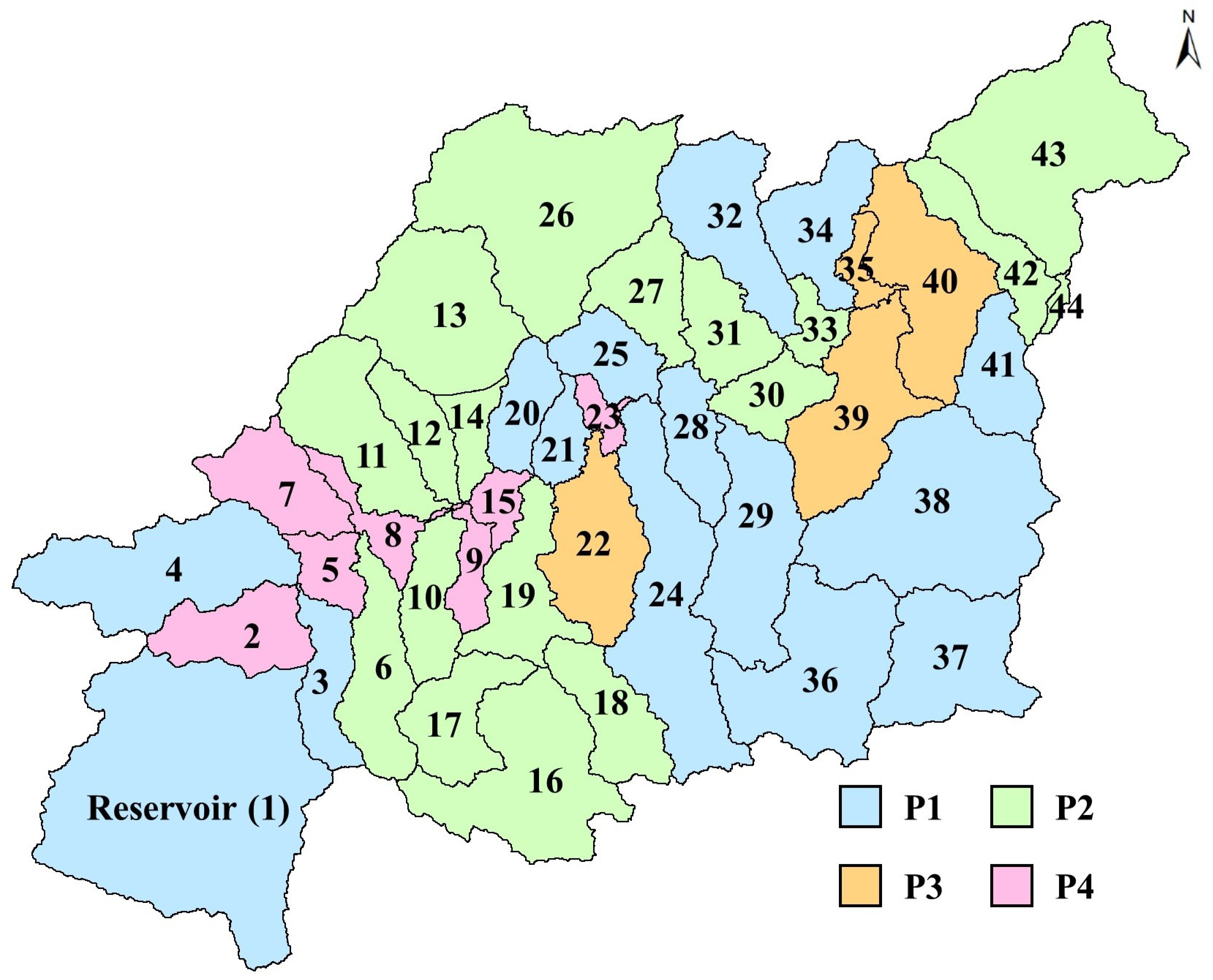
2.4. The Model Calibration and Validation

The river channel raster data (manually converted to an elevation value of −100) were delineated from high-resolution remote sensing imagery (0.5 m × 0.5 m) and integrated into the original DEM using ArcGIS, resulting in a corrected DEM. Based on this corrected DEM, ArcSWAT software (version 10.19) was employed to extract the watershed river network and sub-watershed distribution maps. The upstream catchment areas of the Xia’an Reservoir were considered separate sub-watersheds for calculations. The discharge at the outlet of these sub-watersheds was replaced with the reservoir discharge according to local data records. The percentage of impervious area in each sub-watershed was determined based on the land use type map, calculated as the sum of the water surface area and the developed land area. Daily precipitation and evaporation data for each sub-watershed were calculated using the Thiessen Polygon method [52]. The sub-watersheds were classified into four categories (Figure 4) to achieve more reliable simulations through the parameter regionalization method, which was fully described in a previous study [48].
The 10-year data record for river discharge, reservoir discharge, precipitation, and evaporation data was divided into two parts: the 2013–2020 period was used to acquire the optimal estimates for parameters calibration and the 2020–2022 period was used for validation. Based on the revised model components, Particle Swarm Optimization (PSO) was used to calibrate the parameters of the original and modified XAJ model [53]. The metrics of the coefficient of determination (R2), Nash–Sutcliffe coefficient (NSE), and model bias (BIAS) were adopted to evaluate the performance of the daily model predictions (including the three discharge regimes) against the observed data [54].
All correlation and regression analyses (e.g., R2, NSE, and BIAS) and the modified/original XAJ models were performed in the Visual Studio 2017 framework.

3. Results and Discussion

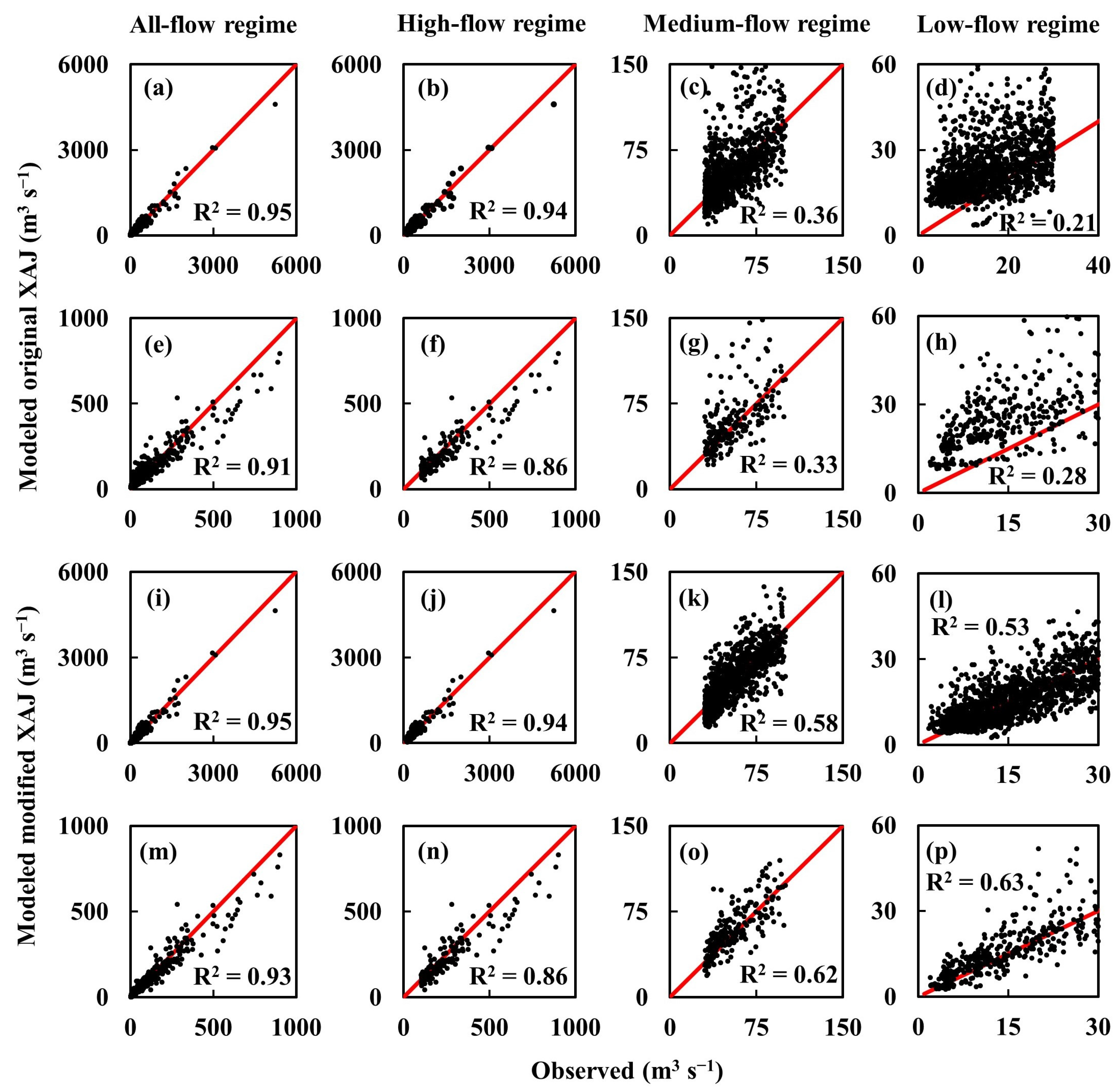
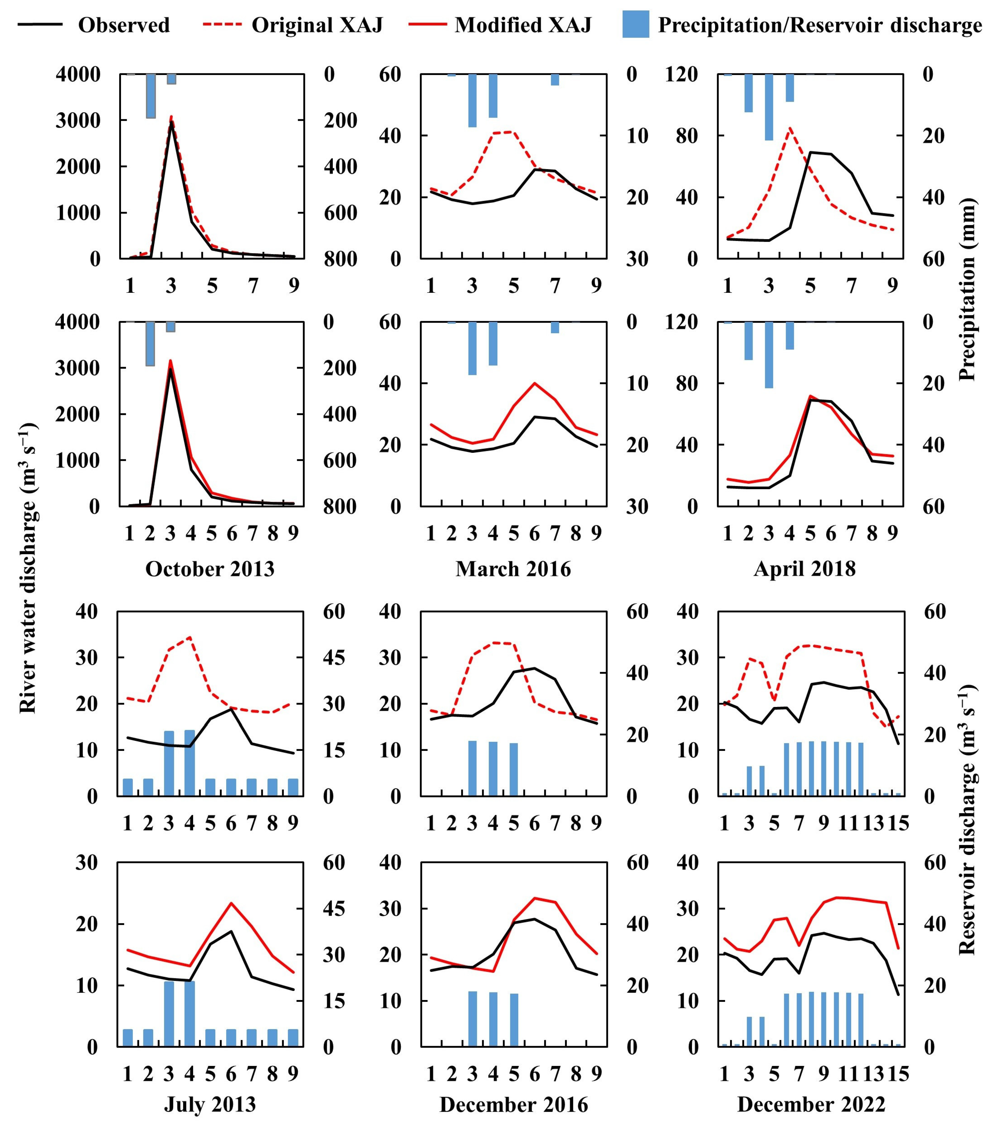
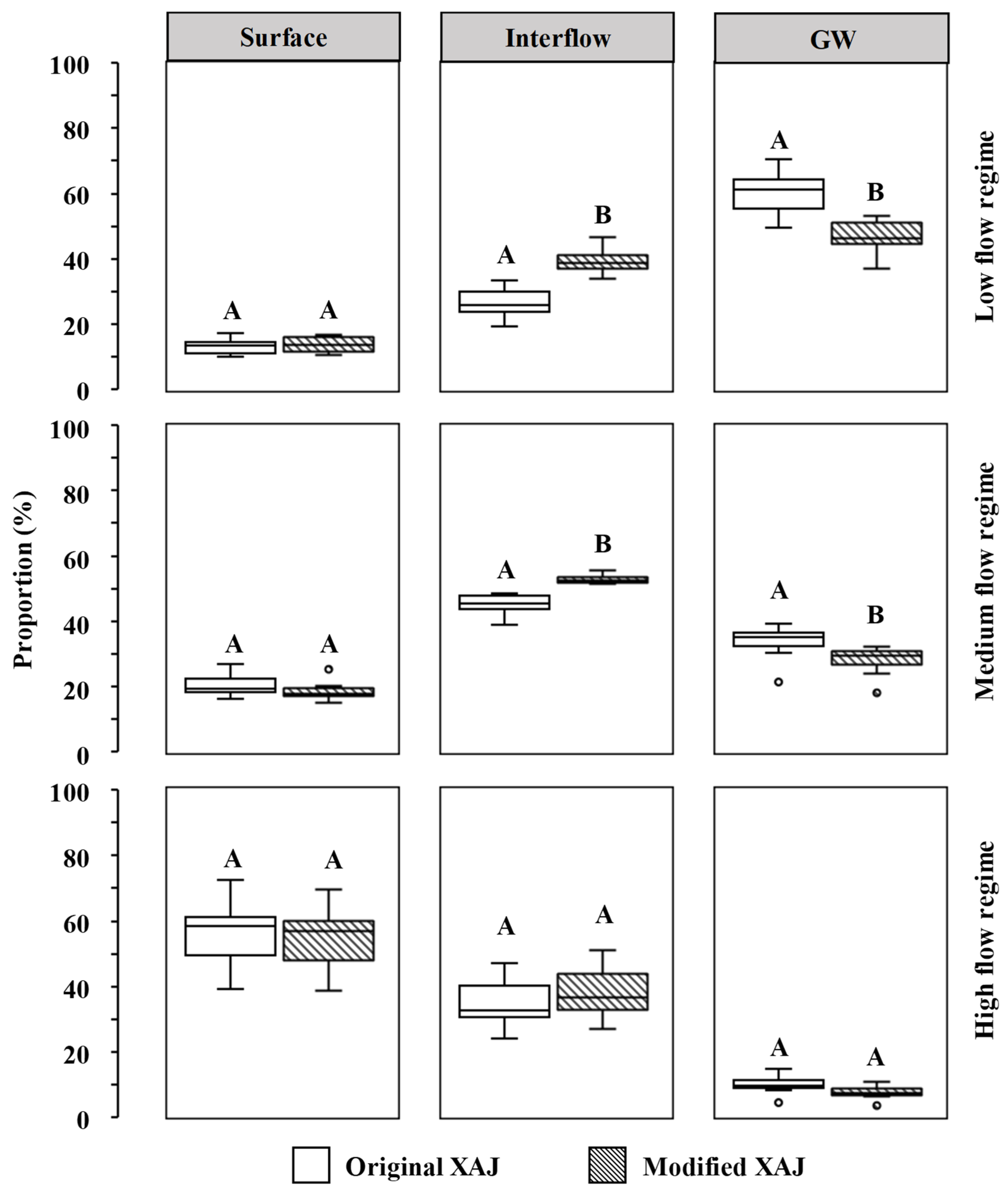
3.1. Performance of the Modified XAJ Model

For the modified XAJ model, the efficiency criteria reached Class A (NSE > 0.90) in accordance with the Standard for Hydrological Information and Hydrological Forecasting of China [55]. The NSE values in this study were comparable to previous applications of the XAJ model in other watersheds (NSE: 0.74–0.97) [36,48,56]. These results confirm that the modified XAJ model effectively captured the hydrological processes in the Yongan River over the 2013–2022 period.
The modified XAJ model achieved high accuracy across all flow regimes during both the calibration (NSE = 0.95, R2 = 0.95) and validation (NSE = 0.92, R2 = 0.93) periods (Table 2 and Figure 5). Although the original XAJ model showed similar performance (NSE = 0.95, R2 = 0.95; NSE = 0.90, R2 = 0.91), its performance was poor during the medium- and low-flow regimes, with NSE coefficients below zero. In comparison, the modified XAJ model improved the simulation results significantly during these periods, with R2 values of 0.53–0.58 and NSE values of 0.40–0.42 during calibration, and R2 values of 0.62–0.63 and NSE values of 0.43–0.46 during validation. Additionally, the BIAS values for the modified XAJ model in the medium- and low-flow regimes decreased from the original range of 7.60% to 89.08% down to 2.06% to 12.72% (Table 2). These patterns indicate that the modified XAJ model significantly improved the simulation performance of medium- and low-flow regimes.
Furthermore, the parameters in the modified XAJ model varied across different flow regimes. Specifically, compared to the high-flow regime, some calibrated parameters showed differences in the low- and medium-flow regimes, with higher values of K parameters (Table 3). We attribute the higher value of the K parameter (ratio of potential evapotranspiration to pan evaporation) in the low- and medium-flow regimes to irrigation water withdrawals, which significantly increase evapotranspiration by providing more water to vegetation [56,57]. Additionally, the proportion of irrigated areas in sub-watersheds P3 and P4 was higher, averaging 41% compared to 19% for P1 and P2. Therefore, the greater parameter changes in sub-watersheds P3 and P4 highlight the impact of irrigation withdrawals. The variations in the K parameter across different flow regimes emphasize the importance of considering both irrigation and in-stream water travel time in hydrological modeling.

3.2. Importance of the Modified Modules

By analyzing hydrometeorological data of the watershed, we selected the typical processes (rainfall and low-flow processes, Figure 6), and examined the temporal characteristics of travel time in the stream channel. Our observations of a typical flood peak process (October 2013 in Figure 6) revealed a one-day delay between rainfall and river discharge, indicating that water traveled through the watershed to the river outlet in one day. Previous studies have shown that during floods, the flood peak can move from upstream to downstream in a few hours [48]. However, during a low-flow regime without precipitation (such as in July 2013 in Figure 6), the discharge at the outlet lagged nearly two days behind the upstream reservoir discharges. This difference in response times between input data (precipitation or reservoir discharge) and output discharge highlights that travel times in the stream channel vary with different rainfall and flow conditions. This is in line with the well-understood hydrologic principle that higher discharges correlate with higher velocities and shorter travel times [51].
The improved simulation performance of the modified XAJ model during the second day of the flood event (October 2013) and during the rising limb under low precipitation (March 2016 and April 2018 in Figure 6) underscores the importance of the modifications. These modifications allowed for an effective transition from dry to wet conditions by accommodating variable travel times, which are crucial when the stream channel is under dry or low-flow conditions. This adjustment is necessary because some catchments may not contribute to streamflow within one day under such conditions [4]. The original XAJ model tended to reflect only the in-stream flow process during high-flow conditions, thus overestimating the influence of distant sub-watersheds on the downstream outlet [58]. It is unrealistic to simulate the rainfall–runoff process across all flow regimes using a single set of parameters [34]. The variable parameter approach has been validated in other studies, significantly enhancing the robustness of model simulations [59].The original XAJ model was primarily designed to capture peak flood data, aiding in the reservoir and flood management with simulation results (NSE and R2) that were reliable and reasonable for most scenarios [48]. However, as the focus expanded to include various flow processes and riverine ecological flows became a critical concern, the need for high-precision simulation across different flow regimes became evident [60]. While some studies introduced efficiency criteria specifically for low-flow simulation, such as NSElnQ, NSEsqrtQ, and the Kling–Gupta efficiency index [54,61], these criteria enhanced the sensitivity of model parameters to low-flow conditions. However, they failed to achieve optimal simulation outcomes for both high- and low-flow regimes using a single parameter set, thus limiting their wider application.
Agricultural irrigation, as the predominant form of water use in agricultural activities, significantly impacts streamflow discharge, particularly in arid and semi-arid regions [43]. However, in the southern mountainous and hilly areas, the effects of agricultural irrigation are often underestimated due to abundant water resources. For instance, in the study area, the annual water consumption for agricultural irrigation averages 80 million cubic meters (Figure 2), which represents less than 4% of the total annual discharge (approximately 2.2 billion cubic meters). Nonetheless, the primary purpose of agricultural irrigation is to ensure that crops receive adequate water for normal growth during dry spells or periods of low rainfall. Specifically, it is assumed that agricultural irrigation occurs only during the no-rainfall conditions, which constitute 60% of the growing season in this study area. Under these conditions, the average daily withdrawals for agricultural irrigation amount to a flow rate of 5.05 m3 s−1, which accounts for approximately 34% of the average streamflow discharge in low-flow regimes.
In the modified XAJ model, the adoption of variable parameter methods significantly improved the model’s ability to accurately track discharge time series phase shifts (Figure 6). Furthermore, incorporating considerations of agricultural irrigation refined the accuracy of amplitude measurements. A notable reduction in BIAS during low-flow conditions (Table 2 and Figure 5) can be attributed to the inclusion of agricultural irrigation withdrawals. Agricultural irrigation practices and water usage vary over time and tend to increase during prolonged periods of water scarcity in the watershed. This increase coupled with extended dry periods further reduces river flow, thus magnifying the influence of irrigation on water use [62]. Unlike previous hydrological models such as SWAT, HYDRUS, and VIC, which often incorporate detailed irrigation management plans or a water stress threshold to enhance simulation accuracy [40,45], this study did not thoroughly examine the relationship between variations in agricultural irrigation and watershed water shortages, primarily due to the lack of detailed irrigation data and soil moisture data. Despite these challenges, the average method employed in this study still yielded significant improvements in simulation accuracy and bias under medium- and low-flow conditions. Therefore, it is posited that more detailed irrigation data could potentially enhance model simulation results further.

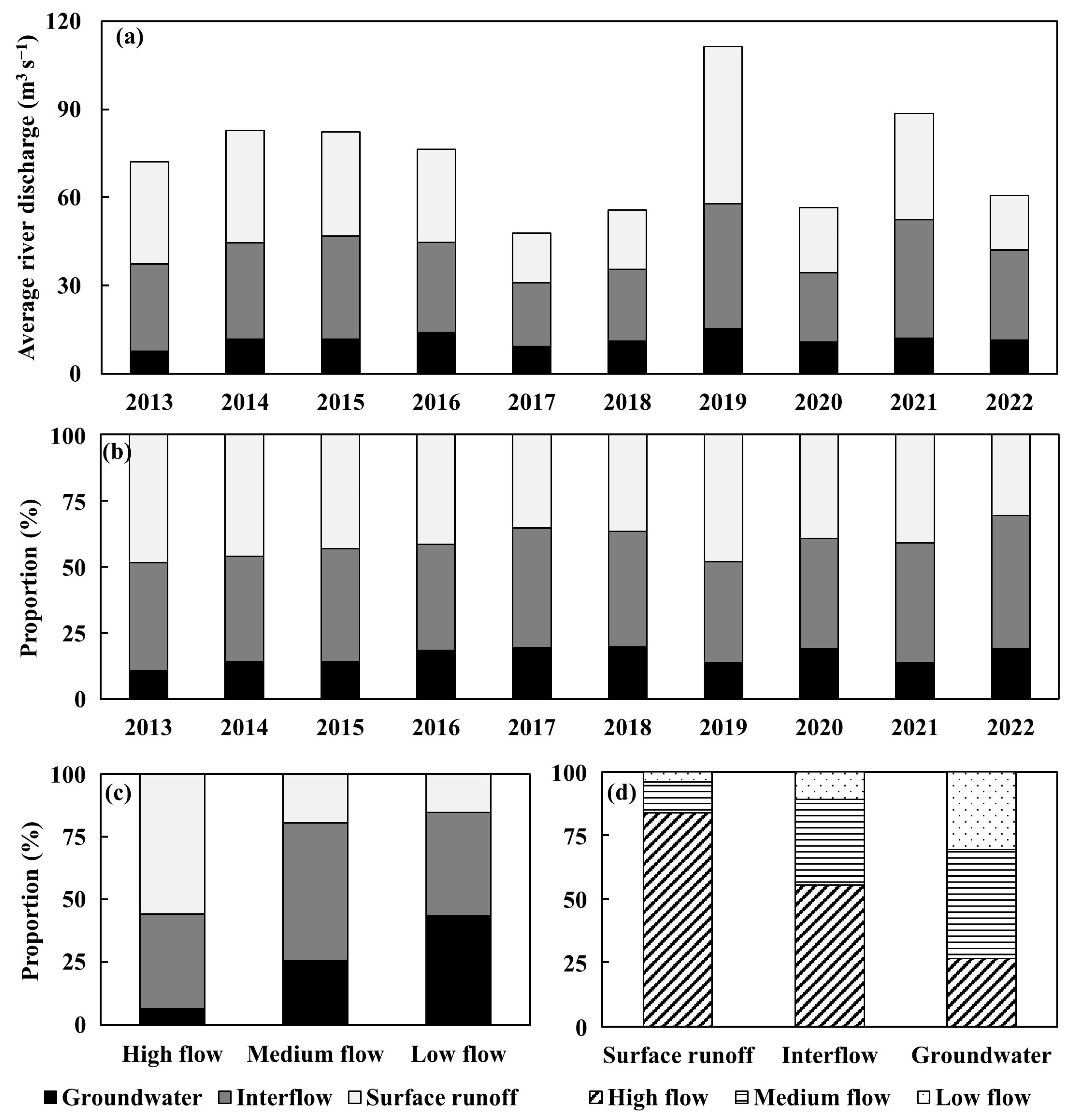
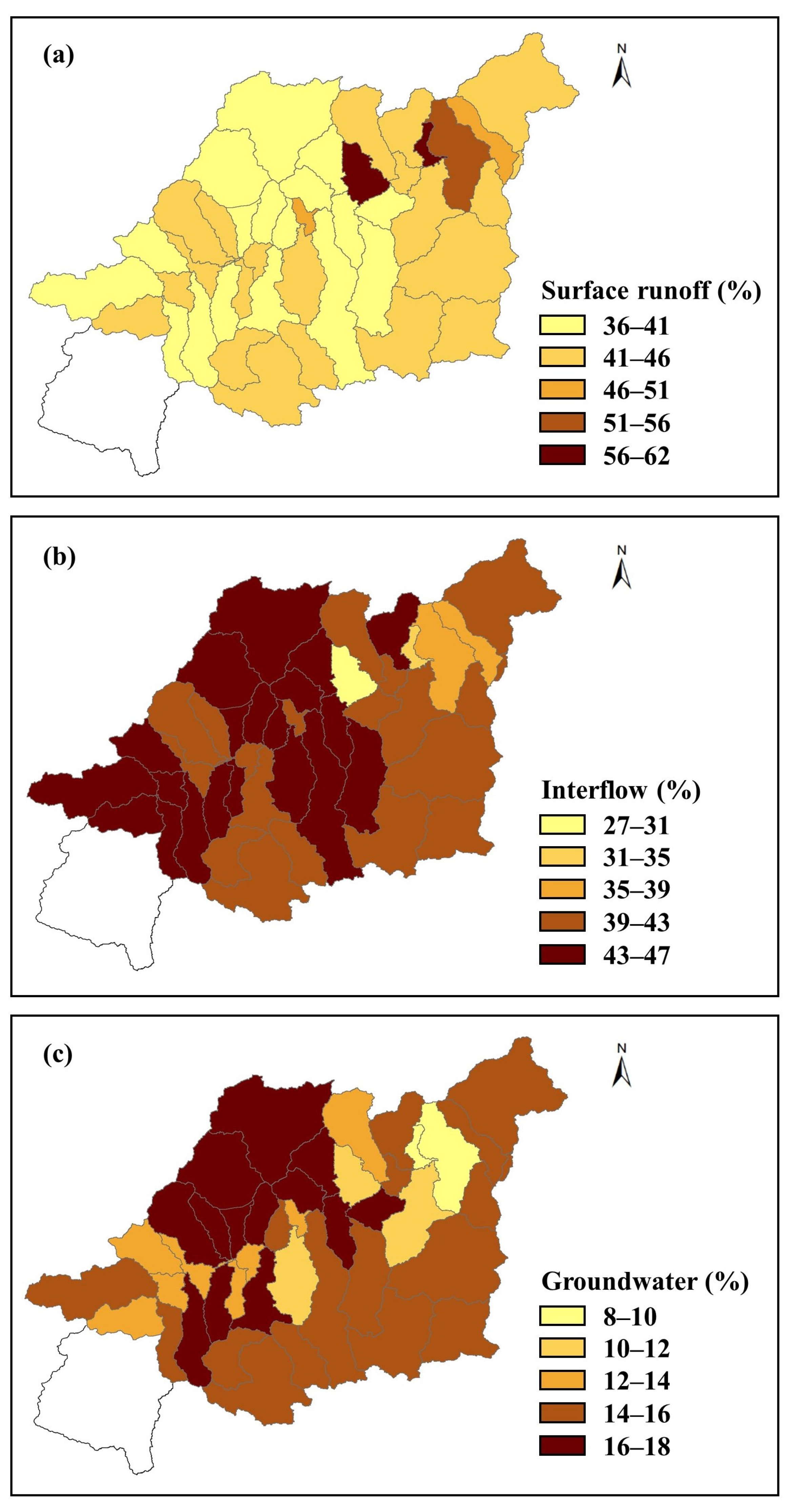
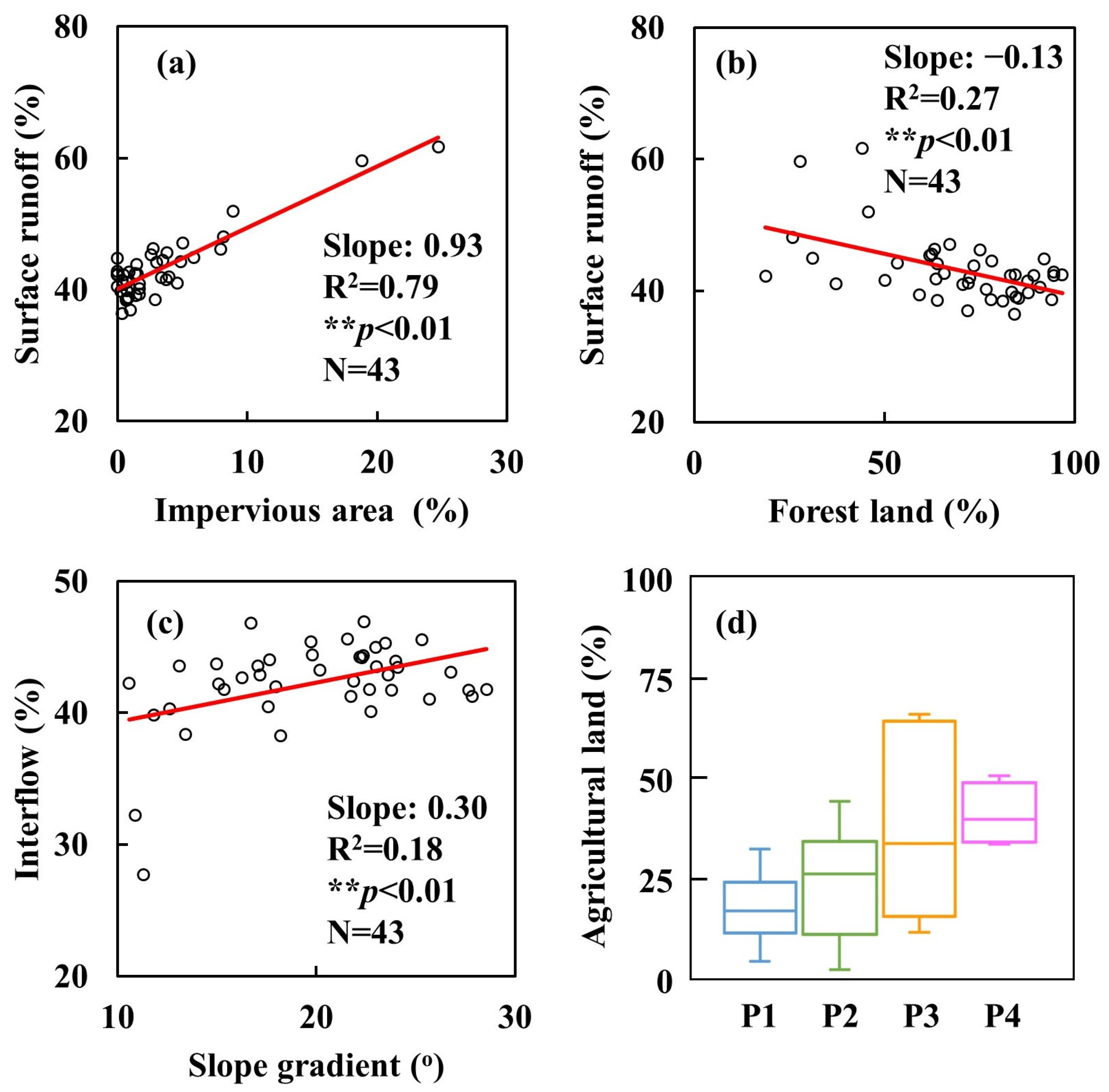
3.3. Temporal and Spatial Variations of Streamflow Components

Based on the improved modeling results, we analyzed the temporal and spatial variations in streamflow components within the Yongan River watershed during the period from 2013 to 2022. Throughout this period, the average daily streamflow discharge at the watershed outlet exhibited significant fluctuations alongside rainfall patterns, ranging from 47.9 to 111.4 m3 s−1. More specifically, surface runoff varied from 16.9 to 53.4 m3 s−1, while interflow and groundwater contributions ranged from 21.7 to 42.6 m3 s−1 and 7.6 to 15.3 m3 s−1, respectively (Figure 7a). Over the decade, at the BZA station located at the watershed outlet, the average contributions of surface runoff, interflow, and groundwater to total streamflow were 42%, 42%, and 16%, respectively.
The contributions of streamflow components across different flow regimes showed significant variations. During high-flow regimes, which typically occur with heavy rainfall events, the streamflow is predominantly composed of surface runoff and interflow, accounting for 56% and 37%, respectively, with groundwater contributing only 7% (Figure 7c). Conversely, in medium-flow regimes, which often represent the recession periods following heavy rainfall or during times of lower precipitation intensity, the proportion of surface runoff decreases sharply to 19%, as the surface runoff quickly exits the watershed via river channel. This predominance of interflow (55%) can be attributed to the high ratio of forest cover (~72%), particularly broadleaf forests, which have a high capacity for water interception and litter production, leading to enhanced soil water infiltration and moisture retention [63,64]. Compared to the highest discharge in 2019, interflow and groundwater proportions were higher in normal and dry years (Figure 7b), reflecting the influence of broadleaf forests [1]. Both high-flow and medium-flow regimes contributed the most surface runoff and interflow (96% and 89%). Meanwhile, the contributions of the three flow regimes to groundwater were relatively similar, at 26%, 43%, and 31% (Figure 7d). This consistency underscores the stability of groundwater, which primarily sustains low-flow conditions and accounts for 44% of the total flow.
The spatial variation in the proportions of surface runoff, interflow, and groundwater estimated using the modified XAJ model was significant, with values ranging from 36% to 62%, 28% to 47%, and 8% to 17%, respectively (Figure 8). From the perspective of watershed categories, the sub-watershed with P1 and P2 generally had a higher proportion of groundwater, while a higher proportion of surface runoff was mainly in the sub-watershed of P4 and P3. Among all the sub-watersheds, the highest proportion of surface runoff (62%) was observed in sub-watershed No. 30, which also featured the largest proportion of impervious area (25%), which was mainly the developed land. Across all sub-watersheds, a strong positive correlation was found between the proportion of impervious area and the estimated proportion of surface runoff (R2 = 0.79, ** p < 0.01, Figure 9a). This correlation suggests that impervious surfaces facilitate the rapid movement of precipitation into the stream channels as surface runoff, resulting in a relatively high proportion of surface runoff [65].
The spatial distribution of the surface runoff proportion is also significantly influenced by the proportion of forest land (Figure 9b). An increase in forest land leads to higher rates of interception and infiltration, which in turn reduce the generation of surface runoff [66]. As surface runoff originating from upper slopes flows downhill, it is absorbed by soils within the forest land, which have higher infiltration capacities, resulting in a lower proportion of surface runoff [67]. In addition, the sub-watershed with the P3 and P4 areas had relatively higher agricultural land proportion (Figure 9d), which might be another reason for the higher surface runoff proportion (Figure 8a). As the primary type of agricultural land in the study area, paddy fields would result in the formation of a plow layer tread that was waterproof [68]. During rainfall events, the waterproof coating on the floor of the paddy cannot infiltrate rainwater, like an impervious area, thereby increasing the dominance of surface runoff [69]. A correlation analysis indicated that the proportion of interflow was positively related to slope gradient (Figure 9c). This relationship is due to higher slope gradients enhancing the potential energy and shearing force of the infiltrated runoff, which subsequently increases the proportion of interflow [70]. However, the results of the modified XAJ model did not show significant correlations with other sub-watershed characteristics, which may be attributed to the complex interactions among these characteristics [3].
There were noticeable differences in the results of the hydrograph separation between the original and modified XAJ models, particularly in the medium- and low-flow regimes (Figure 10). The original XAJ model tended to underestimate the proportion of interflow, averaging 13% in the low-flow regime and 7% in the medium-flow regime, while overestimating the proportion of groundwater at 14% and 6%, respectively. To further analyze these differences, we examined three tributary sub-watersheds with the highest (No. 2, 3, and 34) and lowest (No. 21, 25, and 35) effective irrigated agricultural areas. In the highly irrigated areas, the proportion of groundwater decreased by 9–10%, with a more pronounced decrease of 20–26% in the low-flow regime. Conversely, in the low-irrigated areas, the decrease in groundwater proportion ranged from 6 to 9% (14 to 20% in the low-flow regime). These findings highlight the significant impact of irrigation withdrawals on the spatial distribution of streamflow components in the Yongan River watershed and underscore the critical need for accurate simulation of medium- and low-flow regimes in hydrograph separation.

3.4. Future Developments

The modified XAJ model enhances the accuracy of spatial and temporal river discharge data, particularly in low-flow regimes (Figure 5), providing crucial information for watershed managers to make informed decisions on water resource management. The adoption of the variable parameter method in this study demonstrates that a single set of optimal parameters is insufficient to accurately simulate the entire range of discharge regimes, especially during extreme high and low flows. The modifications were designed based on the hydrological characteristics of our study area, suggesting that further applications in other agricultural watersheds are necessary to validate the model’s applicability and reliability. For example, the division of discharge regimes only based on the discharge at the watershed outlet was relatively reasonable in this study, attributed to relatively consistent rainfall events across the sub-watershed. However, in larger watersheds or those with more varied rainfall, sub-basin rainfall events could independently affect the travel time from the sub-watershed to the outlet [71]. The effects of rainfall events in the sub-watershed require more rainfall data and discharge records at the outlet of the sub-watershed to verify and further improve the calculation of the stream channel process. Additional observational data are essential as intermediate variables to delineate and confirm the hydrological response from sub-watersheds and prevent issues of equifinality [72].
Moreover, due to the limitation of data collection in the study area, the module of agricultural irrigation withdrawals is actually relatively rough on a day scale. Compared to modeled discharges, observed discharges sometimes exhibit abnormal fluctuations, creating a sawtooth hydrograph, which may be attributable to varying daily irrigation water withdrawals [73]. The frequency of these fluctuations is likely to increase with more extensive use of agricultural irrigation water [74]. Incorporating precise planning for agricultural irrigation withdrawals or establishing water stress and soil water deficit thresholds could enable the real-time forecasting of low-flow discharges on a daily scale [40,45]. Such forecasting could provide early warnings of impending low-flow conditions, which are critical for managing water withdrawals, ensuring ecological river discharge, and maintaining water quality [32,33,75].

4. Conclusions

This study introduced two key modifications to the XAJ model aimed at quantifying the spatial and temporal distribution of discharge and streamflow components without substantially increasing the structural complexity or the data demand of the model. These modifications involved adjustments to water travel times within the stream channel and the integration of an irrigation withdrawals module, both of which significantly improved the model’s performance, particularly in low-flow regimes. Although the enhancements in NSE and R2 were not substantial for overall discharge and high-flow regimes, the shift of NSE values from negative to positive in medium- and low-flow regimes indicates that the modified XAJ model significantly improves the accuracy of predictions regarding the fluctuation period and amplitude of discharges in these regimes. This enhanced capability enables decision-makers to more effectively design and implement measures for water resource management. The modified model facilitated a detailed analysis of the spatial and temporal distribution of streamflow discharge and its components, such as surface runoff, interflow, and groundwater. These insights are crucial for improving hydrograph response and separation techniques. The findings enhance our understanding of the hydrological processes and cycles at the watershed scale, particularly for subtropical rivers in eastern China.

Author Contributions

Conceptualization, D.C. and K.W.; methodology, D.C. and K.W.; software, K.W.; validation, D.C. and K.W.; formal analysis, D.C., K.W. and M.H.; investigation, D.C.; resources, D.C.; data curation, K.W., Y.Z. and J.Z.; writing—original draft preparation, K.W.; writing—review and editing, D.C. and M.H.; visualization, K.W.; supervision, D.C.; project administration, D.C.; funding acquisition, D.C. All authors have read and agreed to the published version of the manuscript.

Funding

This work was funded by the National Key Research and Development Program of China (2021YFD1700802) and the National Natural Science Foundation of China (42107393/42177352).

Data Availability Statement

The data presented in this study are available on request from the corresponding author due to privacy.

Acknowledgments

We extend our appreciation to Minpeng Hu for his contributions in refining the language and providing insightful comments on the manuscript, and to Zhiwei Yin and Xihan Wang from the Taizhou City Water Resources Bureau for their investigation.

Conflicts of Interest

The authors declare no conflicts of interest.

References

  1. Ding, B.; Zhang, Y.; Yu, X.; Jia, G.; Wang, Y.; Wang, Y.; Zheng, P.; Li, Z. Effects of Forest Cover Type and Ratio Changes on Runoff and Its Components. Int. Soil Water Conserv. Res. 2022, 10, 445–456. [Google Scholar] [CrossRef]
  2. Klaus, J.; McDonnell, J.J. Hydrograph Separation Using Stable Isotopes: Review and Evaluation. J. Hydrol. 2013, 505, 47–64. [Google Scholar] [CrossRef]
  3. Hu, M.; Liu, Y.; Wang, J.; Dahlgren, R.A.; Chen, D. A Modification of the Regional Nutrient Management Model (ReNuMa) to Identify Long-Term Changes in Riverine Nitrogen Sources. J. Hydrol. 2018, 561, 31–42. [Google Scholar] [CrossRef]
  4. Van Meerveld, H.J.I.; Kirchner, J.W.; Vis, M.J.P.; Assendelft, R.S.; Seibert, J. Expansion and Contraction of the Flowing Stream Network Alter Hillslope Flowpath Lengths and the Shape of the Travel Time Distribution. Hydrol. Earth Syst. Sci. 2019, 23, 4825–4834. [Google Scholar] [CrossRef]
  5. Choi, B.; Kang, H.; Lee, W. Baseflow Contribution to Streamflow and Aquatic Habitats Using Physical Habitat Simulations. Water 2018, 10, 1304. [Google Scholar] [CrossRef]
  6. Liu, Z.; Liu, S.; Ye, J.; Sheng, F.; You, K.; Xiong, X.; Lai, G. Application of a Digital Filter Method to Separate Baseflow in the Small Watershed of Pengchongjian in Southern China. Forests 2019, 10, 1065. [Google Scholar] [CrossRef]
  7. Blume, T.; Zehe, E.; Bronstert, A. Rainfall—Runoff Response, Event-Based Runoff Coefficients and Hydrograph Separation. Hydrol. Sci. J. 2007, 52, 843–862. [Google Scholar] [CrossRef]
  8. Mei, Y.; Anagnostou, E.N. A Hydrograph Separation Method Based on Information from Rainfall and Runoff Records. J. Hydrol. 2015, 523, 636–649. [Google Scholar] [CrossRef]
  9. Zhang, J.; Zhang, Y.; Song, J.; Cheng, L. Evaluating Relative Merits of Four Baseflow Separation Methods in Eastern Australia. J. Hydrol. 2017, 549, 252–263. [Google Scholar] [CrossRef]
  10. He, S.; Li, S.; Xie, R.; Lu, J. Baseflow Separation Based on a Meteorology-Corrected Nonlinear Reservoir Algorithm in a Typical Rainy Agricultural Watershed. J. Hydrol. 2016, 535, 418–428. [Google Scholar] [CrossRef]
  11. Hu, M.; Zhang, Y.; Wu, K.; Shen, H.; Yao, M.; Dahlgren, R.A.; Chen, D. Assessment of Streamflow Components and Hydrologic Transit Times Using Stable Isotopes of Oxygen and Hydrogen in Waters of a Subtropical Watershed in Eastern China. J. Hydrol. 2020, 589, 125363. [Google Scholar] [CrossRef]
  12. Lott, D.A.; Stewart, M.T. Base Flow Separation: A Comparison of Analytical and Mass Balance Methods. J. Hydrol. 2016, 535, 525–533. [Google Scholar] [CrossRef]
  13. Miller, M.P.; Susong, D.D.; Shope, C.L.; Heilweil, V.M.; Stolp, B.J. Continuous Estimation of Baseflow in Snowmelt-dominated Streams and Rivers in the U Pper C Olorado R Iver B Asin: A Chemical Hydrograph Separation Approach. Water Resour. Res. 2014, 50, 6986–6999. [Google Scholar] [CrossRef]
  14. Long, A.J. Hydrograph Separation for Karst Watersheds Using a Two-Domain Rainfall–Discharge Model. J. Hydrol. 2009, 364, 249–256. [Google Scholar] [CrossRef]
  15. Luo, Y.; Arnold, J.; Allen, P.; Chen, X. Baseflow Simulation Using SWAT Model in an Inland River Basin in Tianshan Mountains, Northwest China. Hydrol. Earth Syst. Sci. 2012, 16, 1259–1267. [Google Scholar] [CrossRef]
  16. Yang, W.; Chen, L.; Deng, F.; Lv, S. Application of an Improved Distributed Xinanjiang Hydrological Model for Flood Prediction in a Karst Catchment in South-Western China. J. Flood Risk Manag. 2020, 13, e12649. [Google Scholar] [CrossRef]
  17. Zhao, R. The Xinanjiang Model Applied in China. J. Hydrol. 1992, 135, 371–381. [Google Scholar] [CrossRef]
  18. Yang, X.; Magnusson, J.; Huang, S.; Beldring, S.; Xu, C.-Y. Dependence of Regionalization Methods on the Complexity of Hydrological Models in Multiple Climatic Regions. J. Hydrol. 2020, 582, 124357. [Google Scholar] [CrossRef]
  19. Ahirwar, A.; Jain, M.K.; Perumal, M. Performance of the Xinanjiang Model. In Hydrologic Modeling; Singh, V.P., Yadav, S., Yadava, R.N., Eds.; Water Science and Technology Library; Springer: Singapore, 2018; Volume 81, pp. 715–731. ISBN 978-981-10-5800-4. [Google Scholar]
  20. Nghi, V.V.; Lam, D.T.; Dung, D.D. Comparison of Two Hydrological Model Simulations Using NAM and XINANJIANG for Nong Son Catchment. Vietnam J. Mech. 2008, 30, 43–54. [Google Scholar] [CrossRef]
  21. Yew Gan, T.; Dlamini, E.M.; Biftu, G.F. Effects of Model Complexity and Structure, Data Quality, and Objective Functions on Hydrologic Modeling. J. Hydrol. 1997, 192, 81–103. [Google Scholar] [CrossRef]
  22. Zhang, M.; Wang, J.; Huang, Y.; Yu, L.; Liu, S.; Ma, G. A New Xin’anjiang and Sacramento Combined Rainfall-Runoff Model and Its Application. Hydrol. Res. 2021, 52, 1173–1183. [Google Scholar] [CrossRef]
  23. WMO Manual on Flood Forecasting and Warning. WMO-1072, 142p. Available online: https://library.wmo.int/doc_num.php?explnum_id=4090 (accessed on 4 February 2024).
  24. Xiang, X.; Pan, Z.; Wu, X.; Yang, H. Seamlessly Coupling Hydrological Modelling Systems and GIS through Object-Oriented Programming. JMSE 2023, 11, 2140. [Google Scholar] [CrossRef]
  25. Gui, Z.; Zhang, F.; Chang, D.; Xie, A.; Yue, K.; Wang, H. A General Method to Improve Runoff Prediction in Ungauged Basins Based on Remotely Sensed Actual Evapotranspiration Data. Water 2023, 15, 3307. [Google Scholar] [CrossRef]
  26. Wang, Y.; Zhong, P.; Zhu, F.; Xu, C.; Mo, R.; Xu, S.; Yang, L.; Wang, S. A Modified Xin’anjiang Model and Its Application for Considering the Regulatory and Storage Effects of Small-Scale Water Storage Structures. J. Hydrol. 2024, 630, 130675. [Google Scholar] [CrossRef]
  27. Zhou, Q.; Chen, L.; Singh, V.P.; Zhou, J.; Chen, X.; Xiong, L. Rainfall-Runoff Simulation in Karst Dominated Areas Based on a Coupled Conceptual Hydrological Model. J. Hydrol. 2019, 573, 524–533. [Google Scholar] [CrossRef]
  28. Zhang, K.; Li, Y.; Yu, Z.; Yang, T.; Xu, J.; Chao, L.; Ni, J.; Wang, L.; Gao, Y.; Hu, Y.; et al. Xin’anjiang Nested Experimental Watershed (XAJ-NEW) for Understanding Multiscale Water Cycle: Scientific Objectives and Experimental Design. Engineering 2022, 18, 207–217. [Google Scholar] [CrossRef]
  29. Ju, Q.; Liu, X.; Zhang, D.; Shen, T.; Wang, Y.; Jiang, P.; Gu, H.; Yu, Z.; Fu, X. Application of Distributed Xin’anjiang Model of Melting Ice and Snow in Bahe River Basin. J. Hydrol. Reg. Stud. 2024, 51, 101638. [Google Scholar] [CrossRef]
  30. Tan, Y.; Dong, N.; Hou, A.; Yan, W. An Improved Xin’anjiang Hydrological Model for Flood Simulation Coupling Snowmelt Runoff Module in Northwestern China. Water 2023, 15, 3401. [Google Scholar] [CrossRef]
  31. Fan, Y.; Li, H.; Miguez-Macho, G. Global Patterns of Groundwater Table Depth. Science 2013, 339, 940–943. [Google Scholar] [CrossRef]
  32. Wu, K.; Hu, M.; Zhang, Y.; Zhou, J.; Wu, H.; Wang, M.; Chen, D. Long-Term Riverine Nitrogen Dynamics Reveal the Efficacy of Water Pollution Control Strategies. J. Hydrol. 2022, 607, 127582. [Google Scholar] [CrossRef]
  33. Miller, M.P.; Buto, S.G.; Susong, D.D.; Rumsey, C.A. The Importance of Base Flow in Sustaining Surface Water Flow in the Upper Colorado River Basin. Water Resour. Res. 2016, 52, 3547–3562. [Google Scholar] [CrossRef]
  34. Tian, Y.; Booij, M.J.; Xu, Y.-P. Uncertainty in High and Low Flows Due to Model Structure and Parameter Errors. Stoch Env. Res Risk Assess 2014, 28, 319–332. [Google Scholar] [CrossRef]
  35. Bai, P.; Liu, X.; Liang, K.; Liu, X.; Liu, C. A Comparison of Simple and Complex Versions of the Xinanjiang Hydrological Model in Predicting Runoff in Ungauged Basins. Hydrol. Res. 2017, 48, 1282–1295. [Google Scholar] [CrossRef]
  36. Li, Z.; Lei, X.; Liao, W.; Yang, Q.; Cai, S.; Wang, X.; Wang, C.; Wang, J. Lake Inflow Simulation Using the Coupled Water Balance Method and Xin’anjiang Model in an Ungauged Stream of Chaohu Lake Basin, China. Front. Earth Sci. 2021, 9, 615692. [Google Scholar] [CrossRef]
  37. Ge, X.; Zhang, L.; Shu, J.; Xu, N. Short-Term Hydropower Optimal Scheduling Considering the Optimization of Water Time Delay. Electr. Power Syst. Res. 2014, 110, 188–197. [Google Scholar] [CrossRef]
  38. Bao, H.; Wang, L.; Zhang, K.; Li, Z. Application of a Developed Distributed Hydrological Model Based on the Mixed Runoff Generation Model and 2D Kinematic Wave Flow Routing Model for Better Flood Forecasting. Atmos. Sci. Lett. 2017, 18, 284–293. [Google Scholar] [CrossRef]
  39. Mizukami, N.; Clark, M.P.; Sampson, K.; Nijssen, B.; Mao, Y.; McMillan, H.; Viger, R.J.; Markstrom, S.L.; Hay, L.E.; Woods, R.; et al. mizuRoute Version 1: A River Network Routing Tool for a Continental Domain Water Resources Applications. Geosci. Model Dev. 2016, 9, 2223–2238. [Google Scholar] [CrossRef]
  40. Neitsch, S.L.; Arnold, J.G.; Kiniry, J.R.; Williams, J.R. Soil and Water Assessment Tool Theoretical Documentation Version 2009; Texas Water Resources Institute: College Station, TX, USA, 2011. [Google Scholar]
  41. Taye, M.T.; Haile, A.T.; Fekadu, A.G.; Nakawuka, P. Effect of Irrigation Water Withdrawal on the Hydrology of the Lake Tana Sub-Basin. J. Hydrol. Reg. Stud. 2021, 38, 100961. [Google Scholar] [CrossRef]
  42. Zeng, R.; Cai, X. Analyzing Streamflow Changes: Irrigation-Enhanced Interaction between Aquifer and Streamflow in the Republican River Basin. Hydrol. Earth Syst. Sci. 2014, 18, 493–502. [Google Scholar] [CrossRef]
  43. Wang, Y.; Zhou, Y.; Franz, K.J.; Zhang, X.; Qi, J.; Jia, G.; Yang, Y. Irrigation Plays Significantly Different Roles in Influencing Hydrological Processes in Two Breadbasket Regions. Sci. Total Environ. 2022, 844, 157253. [Google Scholar] [CrossRef]
  44. Sun, Y.; Chen, X.; Chen, X.; Yang, L. Modeling Groundwater-Fed Irrigation and Its Impact on Streamflow and Groundwater Depth in an Agricultural Area of Huaihe River Basin, China. Water 2021, 13, 2220. [Google Scholar] [CrossRef]
  45. Tatsumi, K.; Yamashiki, Y. Effect of Irrigation Water Withdrawals on Water and Energy Balance in the Mekong River Basin Using an Improved VIC Land Surface Model with Fewer Calibration Parameters. Agric. Water Manag. 2015, 159, 92–106. [Google Scholar] [CrossRef]
  46. Wu, M.; Liu, P.; Lei, X.; Liao, W.; Cai, S.; Xia, Q.; Zou, K.; Wang, H. Impact of Surface and Underground Water Uses on Streamflow in the Upper-Middle of the Weihe River Basin Using a Modified WetSpa Model. J. Hydrol. 2023, 616, 128840. [Google Scholar] [CrossRef]
  47. Chen, D.; Hu, M.; Dahlgren, R.A. A Dynamic Watershed Model for Determining the Effects of Transient Storage on Nitrogen Export to Rivers. Water Resour. Res. 2014, 50, 7714–7730. [Google Scholar] [CrossRef]
  48. Liu, L.; Gu, H.; Xu, Y.-P.; Zheng, C.; Zhou, P. Real-Time Flood Forecasting via Parameter Regionalization and Blending Nowcasts with NWP Forecasts over the Jiao River, China. J. Hydrometeorol. 2023, 24, 561–582. [Google Scholar] [CrossRef]
  49. Li, R.; Du, J.; Bian, G.; Wang, Y.; Chen, C.; Zhang, X.; Li, M.; Wang, S.; Wu, S.; Xie, S.; et al. An Integrated Modelling Approach for Flood Simulation in the Urbanized Qinhuai River Basin, China. Water Resour. Manag. 2020, 34, 3967–3984. [Google Scholar] [CrossRef]
  50. Choo, T.H.; Yoon, H.C.; Lee, S.J. An Estimation of Discharge Using Mean Velocity Derived through Chiu’s Velocity Equation. Env. Earth Sci. 2013, 69, 247–256. [Google Scholar] [CrossRef]
  51. Jobson, H.E. Prediction of Traveltime and Longitudinal Dispersion in Rivers and Streams; United States Geological Survey: Reston, VA, USA, 1996.
  52. Thiessen, A.H. Precipitation averages for large areas. Mon. Wea. Rev. 1911, 39, 1082–1089. [Google Scholar] [CrossRef]
  53. Kennedy, J.; Eberhart, R. Particle Swarm Optimization. In Proceedings of the ICNN’95—International Conference on Neural Networks, Perth, WA, Australia, 27 November–1 December 1995; Volume 4, pp. 1942–1948. [Google Scholar]
  54. Althoff, D.; Rodrigues, L.N. Goodness-of-Fit Criteria for Hydrological Models: Model Calibration and Performance Assessment. J. Hydrol. 2021, 600, 126674. [Google Scholar] [CrossRef]
  55. GB/T 22482-2008; Ministry of Water Resources of the People’s Republic of China (MWR) Standard for Hydrological Information and Hydrological Forecasting. Standards Press of China: Beijing, China, 2008.
  56. Zhang, X.; Liu, P.; Cheng, L.; Xie, K.; Han, D.; Zhou, L. The Temporal Variations in Runoff-Generation Parameters of the Xinanjiang Model Due to Human Activities: A Case Study in the Upper Yangtze River Basin, China. J. Hydrol. Reg. Stud. 2021, 37, 100910. [Google Scholar] [CrossRef]
  57. Puma, M.J.; Cook, B.I. Effects of Irrigation on Global Climate during the 20th Century. J. Geophys. Res. 2010, 115, 2010JD014122. [Google Scholar] [CrossRef]
  58. Van Esse, W.R.; Perrin, C.; Booij, M.J.; Augustijn, D.C.M.; Fenicia, F.; Kavetski, D.; Lobligeois, F. The Influence of Conceptual Model Structure on Model Performance: A Comparative Study for 237 French Catchments. Hydrol. Earth Syst. Sci. 2013, 17, 4227–4239. [Google Scholar] [CrossRef]
  59. Tang, Y.; Sun, Y.; Han, Z.; Soomro, S.; Wu, Q.; Tan, B.; Hu, C. Flood Forecasting Based on Machine Learning Pattern Recognition and Dynamic Migration of Parameters. J. Hydrol. Reg. Stud. 2023, 47, 101406. [Google Scholar] [CrossRef]
  60. Pushpalatha, R.; Perrin, C.; Le Moine, N.; Mathevet, T.; Andréassian, V. A Downward Structural Sensitivity Analysis of Hydrological Models to Improve Low-Flow Simulation. J. Hydrol. 2011, 411, 66–76. [Google Scholar] [CrossRef]
  61. Pushpalatha, R.; Perrin, C.; Moine, N.L.; Andréassian, V. A Review of Efficiency Criteria Suitable for Evaluating Low-Flow Simulations. J. Hydrol. 2012, 420–421, 171–182. [Google Scholar] [CrossRef]
  62. Zhang, J.; Guan, K.; Peng, B.; Pan, M.; Zhou, W.; Jiang, C.; Kimm, H.; Franz, T.E.; Grant, R.F.; Yang, Y.; et al. Sustainable Irrigation Based on Co-Regulation of Soil Water Supply and Atmospheric Evaporative Demand. Nat Commun. 2021, 12, 5549. [Google Scholar] [CrossRef] [PubMed]
  63. Jiang, M.-H.; Lin, T.-C.; Shaner, P.-J.L.; Lyu, M.-K.; Xu, C.; Xie, J.-S.; Lin, C.-F.; Yang, Z.-J.; Yang, Y.-S. Understory Interception Contributed to the Convergence of Surface Runoff between a Chinese Fir Plantation and a Secondary Broadleaf Forest. J. Hydrol. 2019, 574, 862–871. [Google Scholar] [CrossRef]
  64. Li, X.; Xiao, Q.; Niu, J.; Dymond, S.; McPherson, E.G.; Van Doorn, N.; Yu, X.; Xie, B.; Zhang, K.; Li, J. Rainfall Interception by Tree Crown and Leaf Litter: An Interactive Process. Hydrol. Process. 2017, 31, 3533–3542. [Google Scholar] [CrossRef]
  65. Xia, C.; Liu, Y.; Meng, Y.; Liu, G.; Huang, X.; Chen, Y.; Chen, K. Stable Isotopes Reveal the Surface Water-Groundwater Interaction and Variation in Young Water Fraction in an Urbanized River Zone. Urban Clim. 2023, 51, 101641. [Google Scholar] [CrossRef]
  66. Ma, X.; Xu, J.; Luo, Y.; Prasad Aggarwal, S.; Li, J. Response of Hydrological Processes to Land-cover and Climate Changes in Kejie Watershed, South-west China. Hydrol. Process. 2009, 23, 1179–1191. [Google Scholar] [CrossRef]
  67. Harden, C.P.; Scruggs, P.D. Infiltration on Mountain Slopes: A Comparison of Three Environments. Geomorphology 2003, 55, 5–24. [Google Scholar] [CrossRef]
  68. Supriatin, L.S.; Basukriadi, A.; Thayeb, M.H.; Soesilo, T.E.B. The Flooding Effect from Rice Cultivation Technique on Infiltration and Water Balance. For. Geo. 2013, 27, 33–44. [Google Scholar] [CrossRef]
  69. Lee, K.-S.; Park, Y.; Shin, W.-J. Hydrograph Separation for a Small Agricultural Watershed: The Role of Irrigation Return Flow. J. Hydrol. 2021, 593, 125831. [Google Scholar] [CrossRef]
  70. Deng, L.; Fei, K.; Sun, T.; Zhang, L.; Fan, X.; Ni, L. Phosphorus Loss through Overland Flow and Interflow from Bare Weathered Granite Slopes in Southeast China. Sustainability 2019, 11, 4644. [Google Scholar] [CrossRef]
  71. Nicótina, L.; Alessi Celegon, E.; Rinaldo, A.; Marani, M. On the Impact of Rainfall Patterns on the Hydrologic Response. Water Resour. Res. 2008, 44, 2007WR006654. [Google Scholar] [CrossRef]
  72. Döll, P.; Berkhoff, K.; Bormann, H.; Fohrer, N.; Gerten, D.; Hagemann, S.; Krol, M. Advances and Visions in Large-Scale Hydrological Modelling: Findings from the 11th Workshop on Large-Scale Hydrological Modelling. Adv. Geosci. 2008, 18, 51–61. [Google Scholar] [CrossRef]
  73. Greve, P.; Burek, P.; Guillaumot, L.; Van Meijgaard, E.; Aalbers, E.; Smilovic, M.M.; Sperna-Weiland, F.; Kahil, T.; Wada, Y. Low Flow Sensitivity to Water Withdrawals in Central and Southwestern Europe under 2 K Global Warming. Environ. Res. Lett. 2023, 18, 094020. [Google Scholar] [CrossRef]
  74. Liu, K.; Bo, Y.; Li, X.; Wang, S.; Zhou, G. Uncovering Current and Future Variations of Irrigation Water Use Across China Using Machine Learning. Earth’s Future 2024, 12, e2023EF003562. [Google Scholar] [CrossRef]
  75. Ionita, M.; Nagavciuc, V. Forecasting Low Flow Conditions Months in Advance through Teleconnection Patterns, with a Special Focus on Summer 2018. Sci. Rep. 2020, 10, 13258. [Google Scholar] [CrossRef]
Figure 1. Location of the Yongan River watershed in China and the Zhejiang Province, including hydrological stations (BZA), the Xia’an Reservoir station, and weather stations.
Hydrology 11 00090 g001
Figure 2. Historical trends for irrigation water consumption and effective irrigated agricultural area in the Yongan River watershed over the 2013–2022 period.
Hydrology 11 00090 g002
Figure 3. The Xinanjiang model structure and modified framework. The red dashed box denotes a modification to the original XAJ model. FSW, MSW, and CSW represent sub-watersheds that are located far from, a middle distance from, and close to the outlet of the watershed. L represents the lag time in the stream channel.
Hydrology 11 00090 g003
Figure 4. The parameter regionalization (four categories) and the number of each sub-watershed for the Yongan River watershed.
Hydrology 11 00090 g004
Figure 5. Model results for daily discharge of the original (ah) and modified (ip) XAJ model showing observed versus modeled values under different flow regimes within calibration (ad,il) and validation (eh,mp) periods.
Hydrology 11 00090 g005
Figure 6. The modeled daily river discharge for the original (red dot) and modified (red line) XAJ model versus observed values (black line) during the typical flood process and the typical low-flow process.
Hydrology 11 00090 g006
Figure 7. The (a) average discharge and (b) proportions of surface runoff, interflow, and groundwater at the outlet of the watershed (2013–2022), estimated using the modified XAJ model in the Yongan watershed. The (c) proportions of streamflow components in three flow regimes, and the (d) contribution of three flow regimes to streamflow components at the outlet of the watershed.
Hydrology 11 00090 g007
Figure 8. Spatial distribution maps of the 10-year average proportion of (a) surface runoff, (b) interflow, and (c) groundwater estimated using the modified XAJ model in the Yongan River watershed. The white area was upstream of the reservoir.
Hydrology 11 00090 g008
Figure 9. Correlation between (a) surface runoff proportion and impervious area, (b) surface runoff proportion and forest land, and (c) interflow proportion and slope gradient in the sub-watershed. (d) The proportion of agricultural land in the four categories of sub-watershed. ** denote significant correlations (p < 0.01).
Hydrology 11 00090 g009
Figure 10. The proportion of surface runoff, interflow, and groundwater estimated using the original and modified XAJ model in low-, medium-, and high-flow regimes. Capital letters above bars denote significant differences (p < 0.01).
Hydrology 11 00090 g010
Table 1. Parameters to be calibrated of the XAJ model.
ParameterPhysical MeaningRange
KRatio of potential evapotranspiration to pan evaporation0.7–1.3
CEvapotranspiration coefficient of the deeper soil layer0.01–0.5
UMAveraged soil moisture storage capacity of the upper layer15–20
LMAveraged soil moisture storage capacity of the lower layer60–90
WMSoil tension water capacity100–150
BExponential of the distribution to tension water capacity0.1–0.5
IMPImpervious areas proportionDefined
SMFree water capacity of the surface soil layer10–50
EXExponent of the free water capacity curve influencing the development of the saturated area1–1.5
KIOutflow coefficients of soil-free water storage to interflow0–0.7
KGOutflow coefficients of soil-free water storage to groundwater0–0.7
CIRecession constants of the lower-interflow storage0–1
CGRecession constants of the lower-groundwater storage0.9–0.999
CRRecession constant in the lag-and-route method for the recession constant for channel routing0–0.1
LEmpirical value of lag timeDefined
Table 2. Calibration and validation performances of the original and modified XAJ model.
ModelCalibrationValidation
AllHighMediumLowAllHighMediumLow
Original XAJR20.950.940.360.210.910.860.330.28
NSE0.950.94−2.59−0.490.900.82−4.43−1.30
BIAS (%)5.03−4.507.6059.213.00−11.5616.4789.08
Modified XAJR20.950.940.580.530.930.870.620.63
NSE0.950.940.420.400.920.830.460.43
BIAS (%)−0.78−2.632.063.55−4.65−10.157.1212.72
All, High, Medium, and Low represent the all-flow regime, high-flow regime (discharge > 100 m3 s−1), medium-flow regime (discharge between 30–100 m3 s−1), and low-flow regime (discharge < m3 s−1), respectively.
Table 3. List of the optimal parameter set calibrated for the modified XAJ model.
High-Flow RegimeMedium-Flow RegimeLow-Flow Regime
ParameterP1P2P3P4P1P2P3P4P1P2P3P4
K1.081.131.070.71.11.251.110.901.11.31.31.00
C0.160.150.150.180.160.150.150.180.160.150.150.18
UM151719181517191815171918
LM707389897073898970738989
WM119124132138119124132138119124132138
B0.220.260.320.310.220.260.320.310.220.260.320.31
SM323531203235312032353120
EX1.21.41.31.21.21.41.31.21.21.41.31.2
KI0.40.410.460.520.40.410.460.520.40.410.460.52
KG0.30.290.240.180.30.290.240.180.30.290.240.18
CI0.780.860.770.780.730.680.640.790.660.780.870.66
CG0.9980.9890.9920.980.9980.9890.9920.980.9980.9890.9920.98
CR0.010.010.020.050.010.010.020.060.020.020.030.05
Disclaimer/Publisher’s Note: The statements, opinions and data contained in all publications are solely those of the individual author(s) and contributor(s) and not of MDPI and/or the editor(s). MDPI and/or the editor(s) disclaim responsibility for any injury to people or property resulting from any ideas, methods, instructions or products referred to in the content.

