Article

Analytical and Numerical Groundwater Flow Solutions for the FEMME-Modeling Environment

1
Civil Engineering Department, Faculty of Engineering, Minia University, Minia 61111, Egypt
2
Civil Engineering Department, College of Engineering, Shaqra University, Dawadmi 11911, Ar Riyadh, Saudi Arabia
3
National Centre for Groundwater Research and Training, College of Science and Engineering, Flinders University, GPO Box 2100, Adelaide, SA 5001, Australia
4
Department of Biology, Ecosystem Management Research Group (ECOBE), University of Antwerp, Universiteitsplein 1, B-2610 Antwerpen, Belgium
5
Water Research Laboratory, School of Civil & Environmental Engineering, UNSW Sydney, Sydney, NSW 2052, Australia
6
Connected Waters Initiative Research Centre, UNSW Sydney, Sydney, NSW 2052, Australia
7
Golder Associates Ltd. 700 2 St. Southwest, Calgary, AB T2P 2W2, Canada
8
Department of Hydrology and Hydraulic Engineering, Vrije Universiteit Brussel, Pleinlaan 2, 1050 Brussels, Belgium
9
Doctoral School of Earth Sciences, University of Pécs, Ifjúság útja 6, H-7624 Pécs, Hungary
*
Author to whom correspondence should be addressed.
Hydrology 2020, 7(2), 27; https://doi.org/10.3390/hydrology7020027
Submission received: 3 April 2020 / Revised: 6 May 2020 / Accepted: 8 May 2020 / Published: 12 May 2020
(This article belongs to the Special Issue Integrated Surface Water and Groundwater Analysis)

Abstract

:
Simple analytical and numerical solutions for confined and unconfined groundwater-surface water interaction in one and two dimensions were developed in the STRIVE package (stream river ecosystem) as part of FEMME (flexible environment for mathematically modelling the environment). Analytical and numerical solutions for interaction between one-dimensional confined and unconfined aquifers and rivers were used to study the effects of a 0.5 m sudden rise in the river water level for 24 h. Furthermore, a two-dimensional groundwater model for an unconfined aquifer was developed and coupled with a one-dimensional hydrodynamic model. This model was applied on a 1 km long reach of the Aa River, Belgium. Two different types of river water level conditions were tested. A MODFLOW model was set up for these different types of water level condition in order to compare the results with the models implemented in STRIVE. The results of the analytical solutions for confined and unconfined aquifers were in good agreement with the numerical results. The results of the two-dimensional groundwater model developed in STRIVE also showed that there is a good agreement with the MODFLOW solutions. It is concluded that the facilities of STRIVE can be used to improve the understanding of groundwater-surface water interaction and to couple the groundwater module with other modules developed for STRIVE. With these new models STRIVE proves to be a powerful example as a development and testing environment for integrated water modeling.

1. Introduction

There is a need to evaluate groundwater-surface water (GW-SW) interaction for water and ecosystem management. This is essential because linkages and feedback between groundwater and surface water systems affect both the quantity and quality of available water required by humans and ecosystems [1,2,3,4]. Therefore, the research topic of GW-SW interaction has gained importance in the last two decades, because of its role in conjunctive use, riparian zone management, and ecohydrology. In addition, understanding the interaction between groundwater and surface water can be important in the determination of migration pathways for contaminants [5]. The hydraulics of groundwater interaction with adjoining streams, canals, and drains is an important aspect of many hydrogeologic systems. Examples are the support of groundwater discharge to stream flow, bank storage attenuation of flood waves, and how groundwater discharge to streams lowers water tables maintains favorable root-zone salinity levels and prevents water logging of soil [6].
A variety of investigation methods have been used to study the hydraulic interaction of stream-aquifer systems including analytical, numerical, chemical, and field methods [7,8,9,10,11]. Recent examples of improved capabilities of MODFLOW [12,13,14] for stream-aquifer interaction are GSFLOW [15], HYDRUS [16,17,18] and unsaturated-zone flow (UZF1) packages [19], MIN3P [20], PARFLOW [21], the integrated water flow model (IWFM) [22], and SWAT-MODFLOW [23]. Numerical, chemical, and field methods have been widely used in different regions [24,25,26,27,28,29,30]. To study the interaction of groundwater and surface water flow in a river and adjacent areas, analytical solutions are often advantageous because of their simplicity. They are more general than site-specific field experiments but yet easier to implement for a particular site than numerical models [6]. In fact, several analytical solutions have been published for evaluation of the interaction of groundwater systems and hydraulically connected surface water bodies such as streams, lakes, reservoirs, drains, and canals. These solutions can be useful for understanding base flow processes, determining aquifer hydraulic properties, and predicting the response of aquifers to changing stream stage. Most of the solutions have been developed for confined and unconfined aquifers, such as [6,31,32,33,34,35,36,37].
The goal of this paper is to develop and test modules for groundwater-surface water interaction as part of the STRIVE (stream river ecosystem) package within the flexible environment for mathematically modelling the environment (FEMME) software [38]. Both numerical and analytical solutions have been developed to evaluate hydraulic interaction of river-aquifer systems. The analytical solutions from [31,32] for an unconfined aquifer and from [33] for a confined aquifer to calculate groundwater heads and discharges of the aquifer are described. The numerical solutions are based on the explicit finite difference approximation of the transient flow equation in a saturated, homogeneous, and isotropic aquifer [39]. A two-dimensional groundwater module for an unconfined aquifer is coupled to a one-dimensional hydrodynamic model [40]. This model was tested for a part of the Aa River, Belgium. Inter-model comparison is performed with MODFLOW. We present the modeling methodologies (FEMME, STRIVE package, hydrodynamic model, analytical and numerical solutions) as well as applications and comparison between analytical and numerical solutions, coupling with a hydrodynamic model, and comparison between STRIVE and MODFLOW.

2. Materials and Methods

2.1. FEMME Modeling Environment and STRIVE Package

FEMME was developed by the Netherlands Institute of Ecology (NIOO) [38]. FEMME is a modeling environment for the development and application of ecological time-dependent processes by using numerical integration of time-dependent differential equations. FEMME is constructed for ecosystem modeling and enables the simulation of different physical, biogeochemical, and transport processes of river ecosystems, like retention or exchange of matter [38,41]. The program is written in FORTRAN; it is designed to implement 0- to multi-dimensional, time-dependent models. FEMME is open source and facilitates the use of pre-defined integration tools in a modular FORTRAN environment [38]. FEMME consists of a wide range of numerical functions as integration, forcing, and calibration functions, as well as data manipulation functions. These technical possibilities allow the user to focus on the scientific part of model development rather than having to deal with complex programming issues. Hence, the environment allows rapid and efficient code development for environmental applications.
The STRIVE-package is a set of modules incorporated in the FEMME environment. It consists of different modules for macrophyte growth, water quality, and hyporheic processes, which can be coupled to form numerical models for specific research questions regarding river ecosystems. Hence, the module for hydrodynamic flow can, e.g., interact with a macrophyte growth routine, which influences the Manning coefficient and therefore the flow simulation. A heat transport module was implemented [42,43] in the STRIVE package for studying the vertical interaction in the hyporheic zone between rivers and aquifers. In this article, the STRIVE package is extended with groundwater modules, which are necessary to understand the interaction between a river and its riparian margin.

2.2. Hydrodynamic Module in STRIVE Package

A hydrodynamic surface water flow module [40] was developed for the STRIVE package and applied for a part of the Aa River, Belgium. The module is based on the Saint-Venant equations for one dimensional unsteady open channel flow [44]. Based on the capabilities of STRIVE, we hypothesize that the implementation of simple analytical and numerical groundwater flow solutions coupled with the hydrodynamic surface water module will allow the investigation of groundwater-river exchange processes in more detail.

2.3. Analytical Solutions for Groundwater-Surface Water Interaction

In this section, analytical solutions [31,32,33] for the interaction between surface water and unconfined and confined aquifers are presented.

2.3.1. Edelman Analytical Solution

We describe here the interaction between a river and a one-dimensional homogeneous semi-infinite and unconfined aquifer, which is bounded at one side by a fully-penetrating stream and below by an impermeable stratum (Figure 1). Under steady-state conditions, the water table in the aquifer and the water level in the river coincide, and there is no flow in or out of the aquifer. A sudden rise in the water level of the river induces a flow from the river towards the aquifer. As a result, the water table in the aquifer starts rising until it reaches the same level as that in the river. The flow from the river to the aquifer is unsteady and one-dimensional.
If the Dupuit approximation, i.e., (a) the equipotential lines are vertical and its consequence; (b) the slope of the groundwater table is equivalent to the hydraulic gradient and is invariant with depth, holds [45], then the flow problem can be described by the partial differential equation:
h t = k b S y 2 h x 2
where kb = T is the transmissivity of the homogeneous aquifer [L2T−1], h is the hydraulic head in the aquifer [L], t is the time [T], x is the distance from the river bank [L], and Sy is the specific yield (−). A general solution to Equation (1) does not exist and integration is possible only for specific boundary conditions [46].
Edelman [31] presented a solution for the case of a sudden change of the water level in the river and a constant water level thereafter, h(x, t) = head.
h ( x , t ) = a ( 1 2 π 0 u e μ 2 d μ )
where h(x, t) is the head in the aquifer [L] at the horizontal coordinate x [L] and time t [T], a is the sudden change in the water level of the river [L], and u is a dimensionless auxiliary variable.
u = x 2 S y / 4 K b t
e r f ( u ) = 2 π 0 u e μ 2 d μ
where erf(u) is the error function, and 1-erf(u) = erfc(u) is the complementary error function. Hence, the head in the aquifer can be formulated:
h ( x , t ) = a e r f c ( u )
The flux in the aquifer per unit length of river at distance x is:
q ( x , t ) = a π K b S y t e u 2
Equation (6) gives the discharge from one side of the river. This equation can also be used if the water level in the river suddenly drops, inducing a flow from the aquifer to the river, resulting in a fall of the water table in the aquifer.

2.3.2. Lockington Analytical Solution

Lockington [32] derived simple analytical solutions for the one-dimensional Boussinesq equation using a weighted residual method. His approach can be applied to both a recharging and dewatering semi-infinite unconfined, homogeneous aquifer with a fully penetrating trench. Only the analytical solution for a recharging aquifer is discussed here (Figure 1) [33].
h = h 0 + ( h 1 h 0 ) ( 1 x λ S y K t ) 1 μ
where h is piezometric head [L], h1 is the water level in the river [L], h0 is the initial water level in the river and aquifer [L], K is the hydraulic conductivity of the aquifer [LT−1], Sy is the specific yield of the aquifer [–], and λ and µ are parameters, which are defined as:
μ = 3 4 ( 1 + N ) + N ( 2 A ) + [ ( 2 A ) 2 ( 1 + 2 N ) + N 2 ( 2 + A ) 2 ] 1 2 4 ( 2 A )
λ 2 = ( 1 + μ ) ( 1 + 2 μ ) 2 μ 2 ( h 0 + h 1 )
where A is a constant defined as:
A = 4 [ h 0 + ( 1 + N ) h 1 ] ( 1 + N ) ( 2 + N ) ( h 1 + h 0 )
In which the exponent N is estimated as in Parlange et al. [47]:
N = 2.27932 3 h 0 ( h 1 + 2 h 0 )
The flux from one side of the river is given by:
q = C r ( h 1 h 0 ) K S y 2 t
where Cr is a recharge coefficient, given by:
C r 2 = ( 1 + 2 μ ) ( h 1 + h 0 ) 2 ( 1 + μ )

2.3.3. Bruggeman Analytical Solution

Bruggeman [33] derived the following general analytical solution:
h ( x , t ) = a 2 n Γ ( 1 + n 2 ) t n 2 e r f c ( u )
where:
u = x 2 S / 4 K b t
S is the storage coefficient of the aquifer (−), and n = 0, 1, 2, 3… depends on the type of the water level change in the river. For n = 0, the change in the water level is assumed to be a sudden change. Similarly, an n value of 1 and 2 indicate a linear and parabolic water level change, respectively. Using the following relationship:
i n e r f c ( 0 ) = 1 2 n Γ ( 1 + n 2 ) ,   n = 1 , 0 , 1 , 2 ,
Equation (14) can be simplified:
h ( x , t ) = a t n 2 i n e r f c ( u ) i n e r f c ( 0 )
The flux is calculated based on Darcy’s law:
q ( x , t ) = a 2 t n 1 2 K b S i n 1 e r f c ( u ) i n e r f c ( 0 )
where:
i n e r f c ( u ) = u n i n 1 e r f c ( u ) + 1 2 n i n 2 e r f c ( u ) , n = 1 , 2 , 3 ,
with:
i 0 e r f c ( u ) = e r f c ( u ) ,
i 1 e r f c ( u ) = 2 π e u 2
For n = 0, a sudden change in the surface water level, Equation (17) simplifies to:
h ( x , t ) = a e r f c ( u )
and Equation (18) for the flux from one side of the aquifer to the river reduces to:
q ( x , t ) =   a π K b S t e u 2

2.4. Numerical Solutions for Groundwater-Surface Water Interaction

Numerical solutions for transient groundwater flow (Equation (24)) are implemented in STRIVE. The solutions are based on the explicit finite difference approximation of transient flow in a saturated, homogeneous, incompressible, and isotropic aquifer [39].
2 h x 2 + 2 h y 2 = S T h t R ( x , y , t ) T
where x and y are the spatial coordinates [L], and R is recharge [L].
In order to solve this diffusion equation (Equation (24)), it is necessary to prescribe boundary and initial conditions [39]. Finite difference approximations for different unsteady-state groundwater flow problems are developed in the following sections.

2.4.1. One-Dimensional Flow in a Confined Aquifer

The explicit finite difference approximation for the head for one-dimensional flow in a confined aquifer can be calculated from the heads at time moment n.
h i n + 1 = h i n + F ( h i + 1 n 2 h i n + h i 1 n )
with:
F = T Δ t / S ( Δ x ) 2
In order to implement Equation (25) in STRIVE, the equation should be written as the rate of change in head:
d h i d t = G ( h i + 1 2 h i + h i 1 )
where G is defined as:
G = T / S ( Δ x ) 2
The criterion for stability of the numerical solution of Equation (25) is F < 0.25. ∆t is the time step [T], ∆x is the size of the grid cell [L], h i n and h i n + 1 are the heads in the center of grid cell i at respectively time step n and n + 1, h i + 1 n , h i 1 n are the heads at times step n in the centers of respectively grid cell i+1 and i−1. The discharge from the river to the aquifer or vice versa is calculated by Darcy’s law:
Q = K A d h d l
where Q is the discharge from or into the aquifer [L3T−1], K is the hydraulic conductivity [LT−1], and A is the cross-sectional area normal to the flow direction [L2].

2.4.2. One and Two-Dimensional Flow in an Unconfined Aquifer

The explicit finite difference approximation for the head at time step n+1 in terms of υ for one-dimensional flow in unconfined aquifers is [39]
υ i n + 1 = υ i n + F υ i n ( υ i + 1 n 2 υ i n + υ i 1 n )
with:
υ = h 2
where F is defined as in Equation (26) but with Sy instead of S.
In order to implement Equation (30) in STRIVE, the equation is written as a time derivative:
d υ i d t = G υ i ( υ i + 1 2 υ i + υ i 1 )
where G is defined as in Equation (28) but with Sy instead of S. Considering a finite set of points on a regularly spaced grid (Figure 2), the explicit finite difference approximation for unconfined two-dimensional flow is:
υ i j n + 1 = υ i j n + F υ i j n ( υ i + 1 , j n + υ i , j + 1 n 4 υ i j n + υ i 1 , j n + υ i , j 1 n )
Here, F is equal to:
F = K Δ t / S y a 2
where a = Δx = Δy.
The formulation in STRIVE is:
d υ i j d t = K υ i j S y a 2 ( υ i + 1 , j + υ i , j + 1 4 υ i j + υ i 1 , j + υ i , j 1 )

3. Application and Discussion

3.1. One-Dimensional Analytical and Numerical Solutions for Confined and Unconfined Aquifers

The implemented one-dimensional analytical and numerical solutions for groundwater heads and discharges in unconfined or confined aquifers are compared as a function of time and distance. The solutions were set up in the STRIVE package for a domain perpendicular to the river to calculate the rise in the head and flow in the unconfined or confined aquifer at a distance x from the river after a sudden water level rise of 0.5 m. Table 1 specifies the details for the unconfined and confined aquifer.
The heads are calculated at the center of cells, and the discharges are calculated using Darcy’s equation at the interface of the cells based on the head calculations for a one-day simulation with a time step of 0.001 day. The results of this application are presented below as a comparison between the analytical and numerical solutions.
Figure 3 shows the numerical solution for one-dimensional transient flow through an unconfined aquifer and the analytical solutions of [31,32] for the heads at different lateral distances from the river at 1.5, 12, and 24 h The differences between the solutions of [31,32] and the numerical one are negligible; the maximum difference is 0.021 m between the Edelman [31] and the numerical solutions, and the root mean squared error (RMSE) is 0.0075 m after 1.5 h. The maximum difference between the Lockington [32] and the numerical solutions was 0.015 m, and the RMSE was 0.0048 m.
Figure 4 shows the match between the three solutions for the discharges at the river-aquifer boundary for a simulation period of 1 day. The maximum difference between the analytical (Edelman [31] and Lockington [32]) and the numerical solutions for the groundwater flux per meter of river length is 0.17 m2 d−1, while the RMSE is 0.1 m2 d−1 at 1.5 h. The difference decreases with time.
The groundwater heads and fluxes simulated with the numerical solution for one-dimensional transient flow in a confined aquifer and the analytical solution of Bruggeman [35] are presented in Figure 5 and Figure 6. Figure 5 shows the relationship between groundwater heads as a function of distance from the river at different times (1.5, 12, 24 h). It is observed that the effect of a 0.5 m sudden rise in the river stage is negligible beyond a distance of 80 m from the river-aquifer boundary. The distance increases with time; at 1.5 h the effect disappears after 50 m and at 24 h it is negligible after 80 m from the river-aquifer boundary. The maximum change in head in the aquifer is attained after one day for locations further than 10 m away from the river. The maximum difference between the numerical and Bruggeman [33] solutions was 0.01 m at 1.5 h.
Figure 6 shows the groundwater flux as a function of distance from the river at different times (1.5, 12, 24 h). It is noticed that the maximum discharges are attained within the first 1.5 h and range from 4.13 to 1.25 m2 d−1 per meter of river length for a location 5 m away from the river-aquifer boundary. The maximum difference between the numerical and Bruggeman solutions was 0.3 m2 d−1 and the RMSE was 0.0145 m at 1.5 h. The accuracy of the numerical solution is mainly determined by the space and time discretization. It is concluded that the results of the analytical solutions of Edelman [31], Lockington [32], and Bruggeman [33] are in a good agreement with the numerical solution.

3.2. Two-Dimensional Numerical Solution in an Unconfined Aquifer

The two-dimensional groundwater module for an unconfined aquifer is applied to the Aa River aquifer, Belgium (based on data from [42,43]) (Figure 7).
The simulated area is simplified to be as Figure 8; it has a length of 1000 m (between weirs 3 and 4 in Figure 7), a width of 200 m, a thickness of 20 m, a hydraulic conductivity Kx and Ky of 10 m d−1, a specific yield Sy of 0.2, and a grid cell size of 10 m. To simplify implementation of the problem in STRIVE, we simulated the reach of 1000 m of the Aa River as a straight line, as shown in Figure 8. The groundwater module developed in STRIVE was applied for two cases of the river boundary conditions. In case 1, the river boundary is estimated by interpolation based on the two head values assigned to the upstream and downstream points of the river. The model was run in steady state by using boundary conditions based on interpolation of heads assigned at the corner cells (a = 10.5 m, b = 10.2 m, c = 10.5 m, d = 10.8 m) (Figure 8). The boundary condition heads are interpolated linearly based on the heads assigned at the corner cells. The initial head everywhere in the aquifer is specified as 10.4 m. A time step of 10 seconds was used for a duration of 1000 days.
The simulated groundwater head and the lateral flows are presented in Figure 9 and Figure 10 respectively. From Figure 9, it is observed that the hydraulic gradient is directed towards the river boundary, due to the selected boundary conditions.
Figure 10 shows in two dimensions the lateral groundwater fluxes obtained from the STRIVE model. The fluxes are directed towards the river (values are negative); the maximum and minimum discharges from the aquifer to the river along the river are respectively 1.49 and 0.74 m3 d−1 at 900 m and 200 m viewed from the upstream boundary respectively.
In the second case, the river boundary is based on water levels from a hydrodynamic surface water model, which is also integrated in STRIVE [40]. The water level in the hydrodynamic surface water model was calculated based on an upstream discharge condition, formulated as a half sine wave (Figure 11). Other boundary conditions and initial conditions are the same as those applied in case 1. The model was run in transient for a period of 30 days with a time step of 1 min and output interval of 1 h. The river boundary values in this case were obtained from the output of the hydrodynamic model.
Figure 12 presents the two-dimensional groundwater heads as simulated with STRIVE for this second case. The groundwater heads are presented at two times, in order to study the effect of the river stages on the groundwater heads in the aquifer and to test the response of the interaction between the river and the aquifer. Figure 12a shows the groundwater heads in the aquifer at 24 h (the beginning of the pulse of the upstream discharge in the river). It is observed that the hydraulic gradient is directed towards the river boundary. Figure 12b presents the groundwater heads in the aquifer at 32 h (the maximum effect of the pulse of the upstream discharge in the river). It is observed that at the river-aquifer boundary, the hydraulic gradient is directed from the river boundary to the aquifer.
In Figure 13, the effect of the river pulse on groundwater heads at different times (24, 32, and 480 h) and at different distances along the river at 100 m (near to the upstream model boundary) are shown. At 24 and 480 h (before the beginning and after the ending of the pulse), there is no effect of the river pulse on the groundwater heads, and the flow is directed towards the river boundary. However, at 32 h, the effect of the river pulse on the groundwater heads in the model appears clearly at the edge of the river-aquifer boundary (30 m) and disappears after a distance of 30 m from the river-aquifer boundary.
The river-aquifer fluxes along the river at 24, 32, and 480 h are shown in Figure 14. At the beginning of the pulse, the Aa River gains water from the aquifer, while at 32 h, the aquifer gains water from the Aa River. The Aa River comes back again to gain water from the aquifer after 480 h. The direction and the rate of flow depend on the difference between the river stage and the groundwater heads.

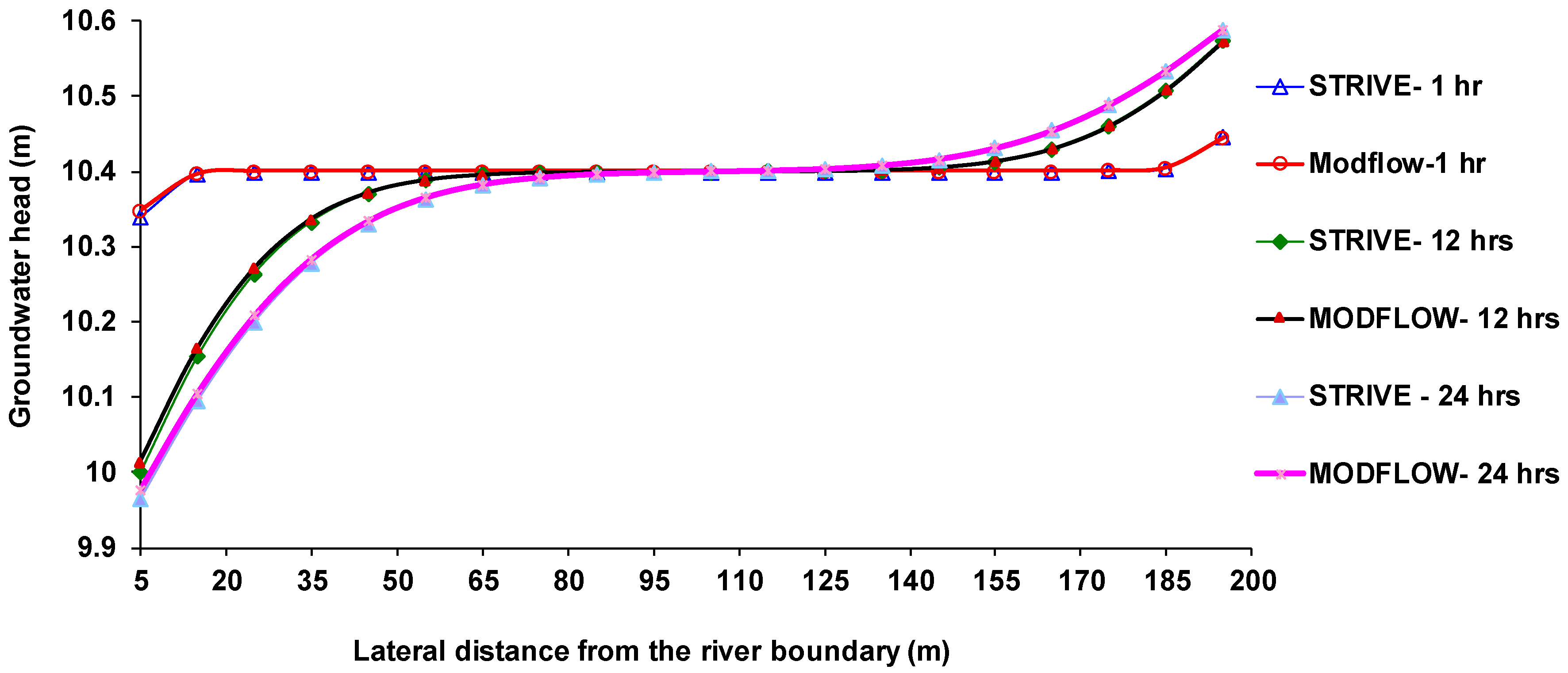
3.3. Comparison between STRIVE and MODFLOW Results

The groundwater flow model MODFLOW-2000 [12] was used for model comparison of the STRIVE two-dimensional groundwater flow implementation. A simple MODFLOW model was set up using the same data as was used for the second case example in STRIVE. The PCG2 solver was used and both steady-state and transient state simulations were performed in order to compare these results with STRIVE results.
In order to see the agreement between the STRIVE and MODFLOW results, the groundwater heads in lateral direction from the river-aquifer boundary at different distances along the river at 5 m (upstream river), 505 m (the middle of the river), and 995 m (downstream river) are shown in Figure 15. Figure 16 shows the groundwater heads in lateral direction from the river-aquifer boundary at distance of 505 m along the river at different simulation times (1, 6, 12, 24 h). The maximum head difference between STRIVE and MODFLOW was 0.004 m, and the RMSE is 7.1 × 10⁻⁶ m and 1.8 × 10⁻⁵ m for steady-state and transient state simulations, respectively.

4. Conclusions

The facilities of STRIVE were tested for the interaction between groundwater flow in confined and unconfined aquifers with streams in one and two dimensions. The analytical solutions implemented in STRIVE include Edelman [31] and Lockington [32] for unconfined aquifers and Bruggeman [33] for confined aquifers. Groundwater heads and discharges in the aquifers were calculated based on a sudden change in the river stage. The results of the analytical solutions were compared with one-dimensional numerical solutions which were implemented in STRIVE for confined and unconfined aquifers. The results of the analytical solutions for confined and unconfined aquifers were in good agreement with the numerical results.
In addition, a two-dimensional groundwater model for an unconfined aquifer was developed in STRIVE and coupled with a one-dimensional hydrodynamic model in STRIVE. This model was applied on a 1 km long reach of the Aa River. The model was tested for two cases with different boundary conditions. In the first case, the river boundary was interpolated, and the model was simulated in steady-state. In the second case, the river boundary was linked with the water levels from a hydrodynamic surface water model. MODFLOW models were set up for these cases as well, in order to check the implementation in STRIVE. The results of the two-dimensional groundwater model developed in STRIVE showed that there is a very good agreement with MODFLOW.
It is concluded that analytical and numerical solutions for groundwater-surface water interaction for unconfined and confined aquifers have been successfully implemented in STRIVE. Hence, STRIVE is extended in terms of modeling facilities for groundwater-surface water interaction, but also due to these implemented sub-models, new integration possibilities with existing modules such as the hydrodynamic, hyporheic zone and sediment appear. The flexibility of STRIVE has proven to be a major advantage in developing these new sub-modules. With these new models, STRIVE increases its capabilities without becoming a dedicated type of model with a graphical user interface. Rather, it is a powerful example of a development and testing environment for integrated water modeling.

Author Contributions

Conceptualization, M.E.-R. and O.B.; methodology M.E.-R., O.B. and K.B.; software, M.E.-R.; K.B.; and C.A.; validation, M.E.-R., O.B. and G.M.; formal analysis, M.E.-R.; O.B.; and K.B.; investigation, M.E.-R.; C.A.; G.M. and W.Z.; data curation, C.A.; G.M.; and W.Z.; writing—original draft preparation, M.E.-R.; writing—review and editing, M.E.-R.; O.B.; K.B; C.A.; W.Z.; and A.S.; visualization, M.E.-R.; and O.B.; supervision, O.B.; K.B.; C.A. and G.M; project administration, O.B. All authors have read and agreed to the published version of the manuscript.

Funding

This research received no external funding.

Conflicts of Interest

The authors declare no conflict of interest.

References

  1. Winter, T.C.; Harvey, J.W.; Franke, O.L.; Alley, W.M. Ground Water and Surface Water: A Single Resource, Circular 1139; U.S. Geological Survey: Reston, VA, USA, 1998; p. 87.
  2. European Commission. E.U. Water Framework Directive, European Parliament and Commission, Official Journal, Directive 2000/60/Ec on 22 December (Directive 2000/60/EC of the European Parliament and of the Council of 23 October 2000 Establishing a Framework for Community Action in the Field of Water Policy); European Commission: Brussels, Belgium, 2000. [Google Scholar]
  3. Sophocleous, M. Interactions between groundwater and surface water: The state of the science. J. Hydrol. 2002, 10, 52–67. [Google Scholar]
  4. Makovníková, J.; Kanianska, R.; Kizeková, M. The ecosystem services supplied by soil in relation to land use. Hung. Geogr. Bull. 2017, 66, 37–42. [Google Scholar] [CrossRef] [Green Version]
  5. Oxtobee, J.P.A.; Novakowski, K. A field study of groundwater/surface water interaction in a fractured bedrock environment. J. Hydrol. 2002, 269, 169–193. [Google Scholar] [CrossRef]
  6. Barlow, P.M.; Moench, A.F. Analytical Solutions and Computer Programs for Hydraulic Interaction of Stream-Aquifer Systems; U.S. Geological Survey: Open-File Report 98-415A; United States Geological Survey: Reston, VA, USA, 1998; p. 85.
  7. Woessner, W.W. Stream and fluvial plain ground water interactions: Rescaling hydrogeologic thought. Ground Water 2000, 38, 423–429. [Google Scholar] [CrossRef]
  8. Moutsopoulos, K.N.; Tsihrintzis, V.A. Approximate analytical solutions of the Forchheimer equation. J. Hydrol. 2005, 309, 93–103. [Google Scholar] [CrossRef]
  9. Kalbus, E.; Reinstorf, F.; Schirmer, M. Measuring methods for groundwater-surface water interactions: A review. Hydrol. Earth Syst. Sci. 2006, 10, 873–887. [Google Scholar] [CrossRef] [Green Version]
  10. Intaraprasong, T.; Zhan, H. A general framework of stream-aquifer interaction caused by variable stream stages. J. Hydrol. 2009, 373, 112–121. [Google Scholar] [CrossRef]
  11. Moutsopoulos, K.N. Solutions of the Boussinesq equation subject to a nonlinear robin boundary condition. Water Resour. Res. 2013, 49, 7–18. [Google Scholar] [CrossRef] [Green Version]
  12. Harbaugh, A.W.; Banta, E.R.; Hill, M.C.; McDonald, M.G. Modflow-2000, the U.S. Geological Survey Modular Ground-Water Model—User Guide to Modularization Concepts and the Ground-Water Flow Process; Open-File Report 00-92; U.S. Geological Survey: Reston, VA, USA, 2000; p. 121.
  13. Harbaugh, A.W. MODFLOW-2005, the U.S. Geological Survey Modular Ground-Water Model—The Ground-Water Flow Process; U.S Geological Survey Techniques and Methods 6-A16; U.S. Geological Survey: Reston, VA, USA, 2005; p. 253.
  14. Niswonger, R.G.; Panday, S.; Ibaraki, M. MODFLOW-NWT, a Newton Formulation for MODFLOW-2005; U.S. Geological Survey: Reston, VA, USA, 2011.
  15. Markstrom, S.; Niswonger, R.; Regan, R.; Prudic, D.; Barlow, P. GSFLOW: Coupled Ground-Water and Surface-Water Flow Model Based on the Integration of the Precipitation-Runoff Modeling System (PRMS) and the Modular Ground-Water Flow Model (MODFLOW-430 2005); U.S. Geological Survey Techniques and Methods 6-d1; U.S. Geological Survey: Reston, VA, USA, 2008; p. 240.
  16. Seo, H.; Šimůnek, J.; Poeter, E. Documentation of the HYDRUS package for MODFLOW-2000, the US geological survey modular ground-water model. IGWMI 2007-01. Integr. In Ground Water Modeling Ctr.; Colorado School of Mines: Golden, CO, USA, 2007; p. 96. [Google Scholar]
  17. Twarakavi, N.K.C.; Šimůnek, J.; Seo, H.S. Evaluating Interactions between Groundwater and Vadose Zone Using the HYDRUS-Based Flow Package for MODFLOW. Vadose Zone J. 2008, 7, 757–768. [Google Scholar] [CrossRef] [Green Version]
  18. Šimůnek, J.; Van Genuchten, M.T.; Šejna, M. Recent Developments and Applications of the HYDRUS Computer Software Packages. Vadose Zone J. 2016, 15, 15. [Google Scholar] [CrossRef] [Green Version]
  19. Niswonger, R.G.; Prudic, D.E.; Regan, R.S. Documentation of the Unsaturated-Zone Flow (UZF1) Package for Modeling Unsaturated Flow between the Land Surface and the Water Table with MODFLOW—2005; US Geological Survey Techniques and Methods 6-A19, Book 6, Chapter A19; USGS: Reston, VA, USA, 2006; 62p.
  20. Mayer, K.; Amos, R.T.; Molins, S.; Gerard, F. Reactive Transport Modeling in Variably Saturated Media with MIN3P: Basic Model Formulation and Model Enhancements. In Groundwater Reactive Transport Models; Zhang, F., Yeh, G.T., Parker, J.C., Shi, X., Eds.; Bentham Science Publishers Ltd.: Sharjah, UAE, 2012; pp. 187–212. [Google Scholar]
  21. Maxwell, R.M.; Kollet, S.J.; Smith, S.G.; Woodward, C.S.; Falgout, R.D.; Ferguson, I.M.; Ferguson, N.; Condon, L.E.; Hector, B.; Lopez, S.; et al. User’s Manual. Integrated GroundWater Modeling Center Report GWMI 2016-01; Free Software Foundation: Boston, MA, USA, 2016; p. 167. [Google Scholar]
  22. Dogrul, E.C. Integrated Water Flow Model. (IWFM–2015): Theoretical Documentation. Modeling Support Branch, Bay-Delta Office, Department of Water Resources: Sacramento, CA, USA, 2016. Available online: http://baydeltaoffice.water.ca.gov/modeling/hydrology/iwfm/iwfm2015/v2015_0_475/downloadables/iwfm-2015.0.475_theoreticaldocumentation.pdf (accessed on 28 September 2016).
  23. Bailey, R.T.; Wible, T.C.; Arabi, M.; Records, R.M.; Ditty, J. Assessing regional-scale spatio-temporal patterns of groundwater–surface water interactions using a coupled SWAT-MODFLOW model. Hydrol. Process. 2016, 30, 4420–4433. [Google Scholar] [CrossRef]
  24. Yang, L.; Song, X.; Zhang, Y.; Han, D.; Zhang, B.; Long, D. Characterizing interactions between surface water and groundwater in the Jialu river basin using major ion chemistry and stable isotopes. Hydrol. Earth Syst. Sci. 2012, 16, 4265–4277. [Google Scholar] [CrossRef] [Green Version]
  25. Tian, Y.; Zheng, Y.; Wu, B.; Wu, X.; Liu, J.; Zheng, C. Modeling surface water-groundwater interaction in arid and semi-arid regions with intensive agriculture, environ. Model. Softw. 2015, 63, 170–184. [Google Scholar] [CrossRef]
  26. El-Rawy, M.; Zlotnik, V.A.; Al-Raggad, M.; Al-Maktoumi, A.; Kacimov, A.; Abdalla, O. Conjunctive use of groundwater and surface water resources with aquifer recharge by treated wastewater: Evaluation of management scenarios in the Zarqa River Basin, Jordan. Environ. Earth Sci. 2016, 75, 1146. [Google Scholar] [CrossRef]
  27. Gannett, M.; Lite, K.J.; Risley, J.; Pischel, E.; La Marche, J. Simulation of Groundwater and Surface-Water Flow in the Upper Deschutes Basin, Oregon, Scientific Investigations Report; U.S. Geological Survey: Portland, OR, USA, 2017; pp. 2017–5097.
  28. Salem, A.; Dezső, J.; Lóczy, D.; El-Rawy, M.; Słowik, M. Modeling surface water-groundwater interaction in an oxbow of the Drava floodplain. In Proceedings of the HIC 2018—13th International Conference on Hydroinformatics, Palermo, Italy, 20 September 2018. [Google Scholar] [CrossRef] [Green Version]
  29. Awad, A.; Eldeeb, H.; El-Rawy, M. Assessment of surface water and groundwater interaction using field measurements: A case study of dairut city, Assuit, Egypt. J. Eng. Sci. Technol. 2020, 1, 406–425. [Google Scholar]
  30. Salem, A.; Dezső, J.; El-Rawy, M.; Lóczy, D. Hydrological Modeling to Assess the Efficiency of Groundwater Replenishment through Natural Reservoirs in the Hungarian Drava River Floodplain. Water 2020, 12, 250. [Google Scholar] [CrossRef] [Green Version]
  31. Edelman, J.H. Over de Berekening van Grondwaterstroomingen (about the Calculation of Groundwater Flow). Ph.D. Thesis, Delft University of Technology, Delft, The Netherlands, 1947. [Google Scholar]
  32. Lockington, D.A. Response of unconfined aquifer to sudden change in boundary head. J. Irrig. Drain. Eng. 1997, 123, 24–27. [Google Scholar] [CrossRef]
  33. Bruggeman, G.A. Analytical Solutions of Geohydrological Problems: Developments in Water Science 46; Elsevier: Amsterdam, The Netherlands; Oxford, UK; New York, NY, USA, 1999; 959p. [Google Scholar]
  34. Cooper, H.; Rorabaugh, M. Groundwater Movements and Bank Storage Due to Flood Stages in Surface Streams; US Government Printing Office: Washington, DC, USA, 1963.
  35. Sahuquillq, A. Quantitative Characterization of the Interaction between Groundwater and Surface Water: Conjunctive Water Use (Proceedings of the Budapest Symposium); IAHS Publ: Wallingford, UK, 1986. [Google Scholar]
  36. Hogarth, W.L.; Parlange, J.Y.; Parlange, M.B.; Lockington, D. Approximation analytical solution of the boussinesq equation with numerical validation. Water Resour. Res. 1999, 23, 3193–3197. [Google Scholar] [CrossRef]
  37. Barlow, P.M.; Moench, A.F. Aquifer response to stream-stage and recharge variations: I. Analytical step-response functions. J. Hydrol. 2000, 230, 192–210. [Google Scholar] [CrossRef]
  38. Soetaert, K.; Declippele, V.; Herman, P.M.J. FEMME, a flexible environment for mathematically modelling the environment. Ecol. Model. 2002, 152, 177–193. [Google Scholar] [CrossRef]
  39. Wang, H.F.; Anderson, M.P. Introduction to Groundwater Modeling: Finite Difference and Finite Element Methods; Academic Press: San Diego, CA, USA, 1995. [Google Scholar]
  40. De Doncker, l.; Troch, P.; Buis, K. A Fundamental Study on Exchange Processes in River Ecosystems: FWO Project, Progress Report, Femme-Modelling; Faculty of Engineering, Ghent University: Ghent, Belgium, 2007. [Google Scholar]
  41. Buis, K.; Anibas, C.; Bal, K.; Banasiak, R.; De doncker, L.; Desmet, N.; Gerard, M.; van belleghem, S.; Batelaan, O.; Troch, P.; et al. Fundamentele studie van uitwisselingsprocessen in rivierecosystemen-geïntegreerde modelontwikkeling (a fundamental study on exchange processes in river ecosystems). Congres Watersysteemkennis, studiedag WSK8 ‘Modellen voor integraal waterbeheer’, Universiteit Antwerpen. Water Tijdschr. Integraal Waterbeleid 2007, 32, 51–54. [Google Scholar]
  42. Anibas, C.; Fleckenstein, J.H.; Volze, N.; Buis, K.; Verhoeven, R.; Meire, P.; Batelaan, O. Transient or steady-state? Using vertical temperature profiles to quantify groundwater–surface water exchange. Hydrol. Process. 2009, 23, 2165–2177. [Google Scholar] [CrossRef]
  43. Anibas, C.; Tolche, A.D.; Ghysels, G.; Nossent, J.; Schneidewind, U.; Huysmans, M.; Batelaan, O. Delineation of spatial-temporal patterns of groundwater/surface-water interaction along a river reach (Aa River, Belgium) with transient thermal modeling. Hydrogeol. J. 2018, 26, 819–835. [Google Scholar] [CrossRef]
  44. Chow, V.T.; Maidment, D.R.; Mays, I.W. Applied Hydrology; Mcgraw-Hill: New York, NY, USA, 1988. [Google Scholar]
  45. Vekerdy, Z.; Meijerink, A.M.J. Statistic and analytical study of the propagation of flood-induced groundwater rise in an alluvial aquifer. J. Hydrol. 1998, 205, 112–125. [Google Scholar] [CrossRef]
  46. De Ridder, N.A.; Zijlstra, G. Seepage and Groundwater Flow; Ritzema, H.P., Ed.; Drainage Principles and Applications; ILRI 16: Wageningen, The Netherlands, 1994; pp. 305–339. [Google Scholar]
  47. Parlange, J.Y.; Barry, D.A.; Parlange, M.B.; Lockington, D.A.; Haverkamp, R. Sorptivity calculation for arbitrary diffusivity. Transp. Porous Media 1994, 15, 197–208. [Google Scholar] [CrossRef]
Figure 1. Unsteady, one-dimensional flow in a semi-infinite unconfined aquifer.
Hydrology 07 00027 g001
Figure 2. A diagram of the finite difference grid cells.
Hydrology 07 00027 g002
Figure 3. Groundwater head versus lateral distance from river at specific times for numerical and analytical solutions (Edelman [31] and Lockington [32]) for a semi-infinite unconfined aquifer.
Hydrology 07 00027 g003
Figure 4. Groundwater discharge versus time at the river-aquifer boundary for numerical and analytical solutions (Edelman [31] and Lockington [32]) for a semi-infinite unconfined aquifer.
Hydrology 07 00027 g004
Figure 5. Groundwater head versus lateral distance from river at specific times for numerical and Bruggeman [33] solutions for a confined aquifer.
Hydrology 07 00027 g005
Figure 6. Groundwater fluxes versus lateral distance from river at specific times (1.5, 12, and 24 h) for numerical and Bruggeman [33] solutions for a confined aquifer.
Hydrology 07 00027 g006
Figure 7. Location and topography map of the Aa River in Belgium.
Hydrology 07 00027 g007
Figure 8. Concept of the groundwater model as simulated with STRIVE and MODFLOW. The heads along the upstream (ad), land side (dc) and downstream (bc) boundaries are specified and interpolated based on four corner heads derived from the original groundwater model (a = 10.5 m, b =10.2 m, c = 10.5 m, d = 10.8 m).
Hydrology 07 00027 g008
Figure 9. Groundwater head obtained from STRIVE for the Aa River based on interpolated river boundary with a steady-state simulation.
Hydrology 07 00027 g009
Figure 10. Lateral groundwater flux obtained from STRIVE implementation for the Aa River based on interpolated river boundary with a steady-state simulation.
Hydrology 07 00027 g010
Figure 11. Analytical hydrograph formulated as a half sine wave introduced in hydrodynamic surface water model.
Hydrology 07 00027 g011
Figure 12. Groundwater head obtained from STRIVE for the Aa River based on the hydrodynamic river boundary with a transient simulation: (a) at the beginning of the pulse (24 h), and (b) at the maximum effect of the pulse (32 h).
Hydrology 07 00027 g012
Figure 13. STRIVE simulated groundwater head versus lateral distance from the river-aquifer boundary at 100 m (near to the upstream model boundary in longitudinal direction of the river), at times 24, 32, and 48 h, using a hydrodynamic river boundary with a transient state simulation.
Hydrology 07 00027 g013
Figure 14. Groundwater discharge at a lateral distance of 10 m of the river-aquifer boundary obtained from STRIVE along the Aa River based on the hydrodynamic river boundary with a transient simulation at times of 24, 32, and 480 h.
Hydrology 07 00027 g014
Figure 15. Groundwater head versus lateral distance from the river-aquifer boundary at fixed distances in the longitudinal direction of the river at 5 m (near the upstream model boundary), 505 m (at the middle of the river length), and 995 m (near the downstream model boundary), using STRIVE and MODFLOW, based on interpolated river boundary with a steady-state simulation.
Hydrology 07 00027 g015
Figure 16. Groundwater head versus lateral distance from the river-aquifer boundary at 505 m from the upstream river for FEMME and MODFLOW, based on interpolated river boundary with a transient simulation.
Hydrology 07 00027 g016
Table 1. Parameters and dimensions of the unconfined and confined aquifer.
ParameterValueDimension
Hydraulic conductivity (K)10m d−1
Storage coefficient (S)0.2(−)
Thickness of the aquifer (b)10m
Specific yield (Sy )0.2(−)
Initial head everywhere in the aquifer10.4m
Head in the river10.9m

