Comparing Rain Gauge and Weather RaDAR Data in the Estimation of the Pluviometric Inflow from the Apennine Ridge to the Adriatic Coast (Abruzzo Region, Central Italy)

Abstract

Accurate knowledge of the rain amount is a crucial driver in several hydrometeorological applications. This is especially true in complex orography territories, which are typically impervious, thus, leaving most mountain areas ungauged. Due to their spatial and temporal coverage, weather radars can potentially overcome such an issue. However, weather radar, if not accurately processed, can suffer from several limitations (e.g., beam blocking, altitude of the observation, path attenuation, and indirectness of the measurement) that can hamper the reliability of the rain estimates performed. In this study, a comparison between rain gauge and weather radar retrievals is performed in the target area of the Abruzzo region in Italy, which is characterized by a heterogeneous orography ranging from the seaside to Apennine ridge. Consequently, the Abruzzo region has an inhomogeneous distribution of the rain gauges, with station density decreasing with the altitude reaching approximately 1500 m a.s.l. Notwithstanding, pluviometric inflow spatial distribution shows a subregional dependency as a function of four climatic and altimetric factors: coastal, hilly, mountain, and inner plain areas (i.e., Marsica). Such areas are used in this analysis to characterize the radar retrieval vs. rain gauge amounts in each of those zones. Compared to previous studies on the topic, the analysis presented the importance of an accurate selection of the climatic and altimetric subregional areas where the radar vs. rain gauge comparison is undertaken. This aspect is not only of great importance to correct biases in radar retrieval in a more selective way, but it also paves the way for more accurate hydrometeorological applications (e.g., hydrological model initialization and quantification of aquifer recharge), which, in general, require the accurate knowledge of rain amounts upstream of a basin. To fill the gap caused by the uneven rain gauge distribution, ordinary Kriging (OK) was applied on a regional scale to obtain 2D maps of rainfall data, which were cumulated on a monthly and yearly basis. Weather radar data from the Italian mosaic were also considered, in terms of rain rate retrievals and cumulations performed on the same time frame used for rain gauges. The period considered for the analysis was two continuous years: 2017 and 2018. The output of the elaborations included raster maps for both radar and interpolated rain gauges, where each pixel contained a rainfall quantity. Although the results showed a general underestimation of the weather radar data, especially in mountain and Marsica areas, they were within the 95% confidence interval of the OK estimation. Our analysis highlighted that the average bias between radar and rain gauges, in terms of precipitation amounts, was a function of altitude and was almost constant in each of the selected areas. This achievement suggests that after a proper selection of homogeneous target areas, radar retrieval can be corrected using the denser network of rain gauges typically distributed at lower altitudes, and such correction can be extended at higher altitudes without loss of generality.

1. Introduction

The distribution of meteorological measurement stations on the Italian national territory is not homogeneous due to the logistical and morphological conditions of the mountain ranges. In particular, such distribution in the Apennine chain, where the study area is focused, is uneven and has a very poor coverage above 1000 m above sea level (a.s.l.) [1,2,3]. This becomes a critical issue, especially when there is the need to have information regarding the amount of precipitation in mountain areas, e.g., to estimate the recharge of aquifers [4].

On one hand, to overcome the issues related to a discrete and sparse distribution of rain gauges of the national and regional monitoring network, the spatial distribution of rainfall can be reconstructed using either traditional interpolation techniques [5,6], such as Thiessen polygons, triangulation with linear interpolation, natural neighbor, inverse weighted distance, or spline, or more advanced ones, such as geostatistics. This wide group of methods is based on the regionalized variable theory [7], stating that values of a specific variable defined in space depend on each other [8,9,10]. According to this theory, measurements include a spatially correlated casual component, the mean value, and the residual nonsystematic error [11,12]. These techniques are physically based, as they take advantage of the spatial variability structures of experimental measurements. In addition, they are implemented in a fashion that ensures optimal and unbiased prediction of the selected variables in areas where they are not measured.

On the other hand, weather RaDAR systems (radio detection and ranging, hereafter named “radar” for simplicity) can represent an alternative solution, as they can provide a spatially seamless estimation of rainfall in near real time. A single weather radar can cover large areas up to 200 km from the radar site with a temporal resolution of 5–10 min and a spatial range resolution ranging from 125 m up to 500 m [13]. Weather radar estimates of near-surface precipitation can be affected by several limiting factors [14], which include partial beam blocking from nearby orography, path attenuation caused by the liquid amount along the radar line of sight, radiofrequency interferences, and cone of silence, i.e., unobserved areas close to the ground. Most of these issues can be reduced and compensated for after the proper processing of radar data [15], delivering filtered and reliable radar data. However, especially in complex orography, weather radar sites are often positioned on mountain peaks [16] to ensure large coverages and prevent mountain blocks with the unavoidable drawbacks of (i) increasing the indirect characteristics of the radar measurement in rain regimes caused by the increased distance between the radar measurement aloft and the surface level and (ii) likely differences in the vertical distribution of hydrometeors (i.e., ice snow/ice is sampled by the radar aloft while liquid rain is falling below close to the surface) that makes the inversion of the radar acquisitions into rain rate more challenging. Several techniques exist to compensate for some of the radar limiting factors [17], although residual errors are difficult to completely zero out.

Despite all the above-mentioned critical factors, weather-radar-derived rainfall datasets are valuable with respect to rain gauge networks because they can potentially reduce the uncertainty about precipitation inflow volumes due to their higher spatial-temporal resolution. Weather radars are currently networked and generally used for weather surveillance, hydrological, and meteorological purposes with a special emphasis on data assimilation [18], in support of civil protection activities [19], as well as to better define the water budget in regional aquifers [20] or in wide catchments [21].

In the present study, the possibility of using an alternative precipitation evaluation technique based on weather radar surveys is analyzed with the possibility of cooperation between different methods. In particular, weather radar measurements from the Italian network are compared to geostatistical estimations obtained through the application of the ordinary Kriging (OK) method to rain gauge measurements. Even though it is the most simplified geostatistical approach, if compared to more sophisticated techniques such as co-Kriging [22,23,24,25] or Kriging with external drift [26,27,28], OK is not influenced by the uncertainty associated with auxiliary variables that are generally not quantified. For this reason, in this case, it is considered appropriate, as the main aim is to compare rainfall data collected by different sources and characterized by different supports.

The selected study area falls within the territory of the Abruzzo region and covers a portion of the Italian territory between the Adriatic coast and the Apennine chain.

Because of limitations in data transfer and huge amounts of weather radar data, only 2 years (2017 and 2018) of annual and monthly datasets were analyzed. For the comparison between the interpolated data from the rain gauge network and the weather radar data, the Abruzzo territory is divided into four homogeneous altimetric/climatic zones, and the mean rainfall amount is calculated for each one of them.

Apart from many hydrological applications focused on the rapid response of hydrological basins, this study is more oriented toward applications of rain infiltration into aquifers, which is a long-term process that scarcely depends on small-scale fluctuations of precipitation in space and time. For this reason, a seasonal evaluation is elaborated; for every climatic zone, both sources of rainfall data are aggregated to a seasonal basis to highlight seasonal trends.

The manuscript first explains the study area and the used methods; then, data are shown and discussed using maps and tables followed by conclusions.

2. Materials and Methods

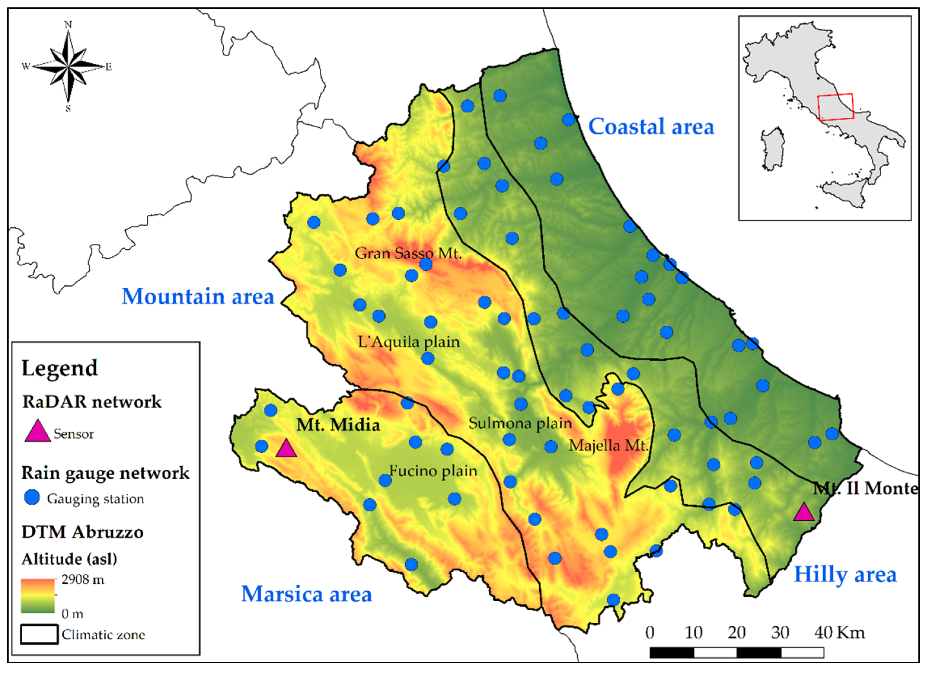
2.1. Study Area and Datasets

The study area is represented by the whole Abruzzo Region with its heterogeneous territory. Its landscape includes mountain areas in the western part and hillier and flatter areas in the eastern (Figure 1); these different morphological features imply different meteorological and pluviometric conditions [29,30].

For these reasons, the study area was divided into four zones on the basis of different altitudes, climatic conditions, and morphological characteristics (Figure 1):

• Coastal area, from sea level to approximately 300 m a.s.l., mainly including the river plains and the seacoast land;
• Hilly area, from approximately 300 to 900 m a.s.l., comprising the hills behind the plains and the lower peaks;
• Mountain area, from approximately 900 m to 3000 m a.s.l., with drainage to the eastern side of the study area (Adriatic Sea), including the main peaks, usually corresponding to the major recharge area, where the Sulmona and L’Aquila plains can also be found;
• Marsica area, with drainage to the western side of the study area (Tyrrhenian Sea), which includes the Fucino plain and nearby mountains.

This subdivision allows correlating precipitations to land features for more accurate data comparison.

Furthermore, considering each zone separately enables highlighting the differences inside the rain gauge network; the coastal and hilly areas are the most homogeneous in station distribution, while the mountain and Marsica ones show a consistent lack of station distribution. As can be seen in Figure 1, automatic stations are mainly located in the flat areas (i.e., Fucino and Sulmona plains), leaving the peaks (i.e., Majella massif) completely uncovered; the higher number of gauges in the mountain area reflects the larger size of that area.

The annual and monthly rainfall datasets (mm; accuracy ± 0.1 mm [1]) used for this paper derive from the regional rain gauge network, managed by the Hydrographic Service of the Abruzzo Region; 72 stations were selected for 2017 and 2018 as they were the only ones with complete monthly data for the considered period (Figure 1 and

Table 1. Numbers of stations for every climatic zone used for ordinary Kriging.

Climatic Zone	Number of Gauging Stations
Coastal area	19
Hilly area	17
Mountain area	27
Marsica area	9

).

Furthermore, in the Abruzzo region, there are four radar sensors installed, but only two of them converge into the national radar mosaic used in this study: Mt. Il Monte and Mt. Midia radars (pink triangles in Figure 1). Mosaicked data were processed to produce monthly and annual cumulative datasets of precipitation.

2.2. Geostatistical Method

The ordinary Kriging (OK) technique [8,9,11] was selected to spatialize rainfall data sampled at the gauging station of the Abruzzo Region monitoring network (Figure 1). In OK, the selected target variable (${\mathrm{z}}^{*}\left(x_0\right)$) can be calculated at each location of a domain grid ($x_0$) through an unbiased and optimal estimator, namely, the best linear unbiased estimator (BLUE), described by the following equation:

$${\mathrm{z}}^{*}\left(x_0\right)={\displaystyle \sum }_{\mathrm{i}=1}^{\mathrm{N}}{\mathsf{\lambda }}_{\mathrm{i}}\mathrm{z}\left(x_{\mathrm{i}}\right) \mathrm{with} \mathrm{i}=1,\dots ,\mathrm{N},$$

(1)

where ${\mathsf{\lambda }}_{\mathrm{i}}$ denotes the weights attributed to the variable values ($\mathrm{z}\left(x_{\mathrm{i}}\right)$) measured at specific locations in the neighborhood ($x_{\mathrm{i}}$).

BLUE ensures that the estimated values are the most optimal and unbiased (i.e., $E\left({\mathrm{z}}^{*}\left(x_0\right)-\mathrm{z}\left(x_0\right)\right)=0$) possible by imposing the following condition:

$${\displaystyle \sum }_{\mathrm{i}}{\mathsf{\lambda }}_{\mathrm{i}}=1.$$

(2)

This constraint is included in the Kriging equation system (Equation (3)), which consists of a set of $\mathrm{N}+1$ linear equations, as shown below:

$$\{\begin{array}{c}{\displaystyle {\displaystyle \sum }_{\mathrm{j}=1}^{\mathrm{N}}}{\mathsf{\lambda }}_{\mathrm{i}}\mathsf{\gamma }\left(x_{\mathrm{i}},x_{\mathrm{j}}\right)+\mathsf{\mu }=\mathsf{\gamma }\left(x_{\mathrm{i}},x_0\right)\\ {\displaystyle {\displaystyle \sum }_{\mathrm{j}=1}^{\mathrm{N}}}{\mathsf{\lambda }}_{\mathrm{j}}=1 \end{array}$$

(3)

where $\mathsf{\mu }$ is a Lagrangian multiplier, whereas $\mathsf{\gamma }\left(x_{\mathrm{i}},x_{\mathrm{j}}\right)$ and $\mathsf{\gamma }\left(x_{\mathrm{i}},x_0\right)$ are the semi-variograms (or variograms) related to pairs of measurements and to pairs that include the unsampled location ($x_0$).

In geostatistics, the variogram is a function that describes the spatial dependency of a given random variable of interest [31] as a relation between semi-variance ($\mathsf{\gamma }\left(h\right)$) and distance, described by a separation vector called lag ($h$). Variograms are defined by the following equation (Equation (4)):

$$\mathsf{\gamma }\left(h\right)=\frac{1}{\mathrm{N}\left(h\right)}{\displaystyle \sum }_{\mathrm{i}=1}^{\mathrm{N}\left(h\right)}{\left[\mathrm{z}\left(x_{\mathrm{i}}\right)-\mathrm{z}\left(x_{\mathrm{i}}+h\right)\right]}^2 \mathrm{with} \mathrm{i}=1,\dots ,\mathrm{N}\left(h\right),$$

(4)

where $\mathrm{z}\left(x_{\mathrm{i}}\right)$ and $\mathrm{z}\left(x_{\mathrm{i}}+h\right)$ are a pair of distinct measurements separated by a lag $h$ regarding a specific location within the considered domain ($x_{\mathrm{i}}$), while $\mathrm{N}\left(h\right)$ is the number of pairs separated by the same lag.

To solve the linear equation system in Equation (3), the experimental variogram (i.e., the one obtained from actual measurements) is fitted by a variogram model, which can be either simple (i.e., one spatial structure) or nested (i.e., two or more spatial structures).

In addition to the predicted value, OK provides a measure of the uncertainty associated with the estimate, namely, the Kriging variance (${\mathsf{\sigma }}^2\left(x_0\right)$), as follows:

$${\mathsf{\sigma }}^2\left(x_0\right)=\mathsf{\mu }+{\displaystyle \sum }_{\mathrm{i}=1}^{\mathrm{N}}{\mathsf{\lambda }}_{\mathrm{i}}\mathsf{\gamma }\left(x_{\mathrm{i}},x_0\right).$$

(5)

In the case of variables characterized by a non-Gaussian statistical distribution, the prediction may be nonlinear and then not optimal, and the Kriging variance or the corresponding standard deviation cannot be used as a local measure of error [32]. For this reason, the yearly and monthly rainfall data were transformed through a well-known function in geostatistics: Gaussian anamorphosis [10]. This function can convert a Gaussian variable ($\mathrm{Z}=\mathsf{\Phi }\left(\mathrm{Y}\right)$) into a non-Gaussian one by fitting a polynomial expansion, as defined in Equation (6).

$$\mathsf{\Phi }\left(\mathrm{Y}\right)={{\displaystyle \sum }}^{ }{\mathsf{\Psi }}_{\mathrm{i}}{\mathrm{H}}_{\mathrm{i}}\left(\mathrm{Y}\right)$$

(6)

Here, ${\mathrm{H}}_{\mathrm{i}}\left(\mathrm{Y}\right)$ denotes the Hermite polynomials, while ${\mathsf{\Psi }}_{\mathrm{i}}$ denotes the Hermite coefficients.

Once defined, this function can be inverted and used to transform a non-Gaussian variable into a standardized one (Equation (7)).

$$\mathrm{Y}={\mathsf{\Phi }}^{-1}\left(\mathrm{Z}\right)$$

(7)

In this study, raw rainfall data were previously transformed into standardized Gaussian variables and then interpolated. Finally, the predictions were back-transformed to obtain the yearly and monthly rainfall maps with the origin unit through the Gaussian anamorphosis function. Back-transformation was also applied to 95% confidence interval limits (lower limit—LL and upper limit—UL) maps, obtained via the following relationship:

$$\mathrm{Limits} \mathrm{of} 95\% \mathrm{CI}={\mathrm{z}}^{*}\left(x\right)\pm \frac{1.96\mathsf{\sigma }}{\sqrt{\mathrm{n}}},$$

(8)

where $\mathsf{\sigma }$ is the OK standard deviation, while $\mathrm{n}$ is the optimal number of measurement locations in the neighborhood.

The performance of selected variogram models used in the OK analyses was evaluated using the cross-validation, which consists of sequentially removing the measurements one at a time and estimating each one of them at the corresponding sampling location, using the model under evaluation and the experimental data in the neighborhood. The differences between measured values and estimates represent errors, from which it is possible to calculate the following performance evaluation statistics, with their reference value:

$$\mathrm{Mean} \mathrm{Error}=\mathrm{ME}=\frac{1}{\mathrm{N}}{\displaystyle \sum }_{\mathrm{i}=1}^{\mathrm{N}}\left({\mathrm{z}}_{\mathrm{i}}^{*}-{\mathrm{z}}_{\mathrm{i}}\right)\to 0,$$

(9)

$$\mathrm{Mean} \mathrm{Standardized} \mathrm{Error}=\mathrm{MSE}=\frac{1}{\mathrm{N}}{\displaystyle \sum }_{\mathrm{i}=1}^{\mathrm{N}}\left(\frac{{\mathrm{z}}_{\mathrm{i}}^{*}-{\mathrm{z}}_{\mathrm{i}}}{{\mathsf{\sigma }}_{\mathrm{i}}}\right)\to 0,$$

(10)

$$\mathrm{Root} \mathrm{Mean} \mathrm{Squared} \mathrm{Error}=\mathrm{RMSE}=\sqrt{\frac{1}{\mathrm{N}}{\displaystyle \sum }_{\mathrm{i}=1}^{\mathrm{N}}{\left({\mathrm{z}}_{\mathrm{i}}^{*}-{\mathrm{z}}_{\mathrm{i}}\right)}^2}\to 0,$$

(11)

$$\mathrm{Root} \mathrm{Mean} \mathrm{Squared} \mathrm{Standardized} \mathrm{Error}=\mathrm{RMSSE}=\sqrt{\frac{1}{\mathrm{N}}{\displaystyle \sum }_{\mathrm{i}=1}^{\mathrm{N}}{\left(\frac{{\mathrm{z}}_{\mathrm{i}}^{*}-{\mathrm{z}}_{\mathrm{i}}}{{\mathsf{\sigma }}_{\mathrm{i}}}\right)}^2}\to 1,$$

(12)

where ${\mathrm{z}}_{\mathrm{i}}^{*}$ and ${\mathrm{z}}_{\mathrm{i}}$ are the estimated and measured values, $\mathrm{N}$ is the number of sampled locations, and ${\mathsf{\sigma }}_{\mathrm{i}}$ is the Kriging standard deviation.

$\mathrm{ME}$ and $\mathrm{MSE}$ measure the variogram model unbiasedness, $\mathrm{RMSE}$ measures its precision, and $\mathrm{RMSSE}$ measures its accuracy.

The rainfall values were estimated by OK through Equation (1) on the same grid (i.e., support) as the weather radar rasters (cell size of 1000 × 1000 m), to make the comparison reliable. Eventually, the output rasters were sliced into the four altimetric zones, rain data were sampled from every pixel, and the mean rainfall amount was calculated for each zone.

All geostatistics analyses were preformed using the software Geovariances Isatis.neo 2021.07 (www.geovariances.com/en/software/isatis-neo-geostatistics-software/).

2.3. Weather RaDAR Method

Weather radars are active instruments that emit electromagnetic (EM) waves, typically in the microwave spectrum and, after the interaction of the EM signal sent with hydrometeors in the atmosphere, the reception of the backscattered component is used to infer some key geophysical information (e.g., hydrometeor typology such as rain, hail, show, water content, and rain rate). Single polarized radars allow the reception of the backscattered power in one single polarization, typically the horizontal one (h), to derive the reflectivity factor (Z_hh), which is strongly dependent on the sixth power of the size of hydrometeors intercepted along the radar ray path. After a proper calibration and processing, Z_hh is converted into instantaneous surface rainfall intensity (S_R), expressed in (mm/h) using the following power law equation:

$${\mathrm{S}}_{\mathrm{R}}={\left({10}^{\frac{{\mathrm{Z}}_{\mathrm{hh}}}{10}}\right)}^{\frac{1}{\mathrm{b}}}{\left(\frac{1}{\mathrm{a}}\right)}^{\frac{1}{\mathrm{b}}},$$

(13)

where a and b are two-dimensional coefficients geographically calibrated [14], and Z_hh is conventionally expressed in mm⁶·m⁻³. ${\mathrm{S}}_{\mathrm{R}}$ is then converted into hourly accumulation by assuming constant rain within the time elapsed between two consecutive radar acquisitions, such that hourly precipitation (P_1h) is:

$${\mathrm{P}}_{1\mathrm{h}}={\displaystyle \sum }_{\mathrm{t}=1}^{\mathrm{N}}{\mathrm{S}}_{\mathrm{R}}\left(\mathrm{t}\right)\Delta \mathrm{t},$$

(14)

where $\Delta \mathrm{t}$ is the time sampling of the radar in (h), and N is the number of the radar acquisitions in the hour considered. Larger accumulation periods are obtained by summing the needed number of hours. It is worth mentioning that dual-polarized radars are multivariable systems adding more information on the shape and composition of hydrometeors, allowing Equation (13) to be constrained to obtain more accurate rain estimates [33]. In addition, these systems allow a better discrimination of the unwanted radar returns, thus, achieving a better data quality, which also indirectly contributes to the accuracy of ${\mathrm{S}}_{\mathrm{R}}$ [17].

The C-band weather radar data used in this work came from the Italian mosaic for a 2017–2018 period with a temporal resolution of $\Delta \mathrm{t}$ = 10 min and the raster representation with a grid spacing of 1 $\times$ 1 km². For the Abruzzo territory, the main contributing radars were those of Il Monte (lon = 14.621°, lat = 41.939°, alt = 710 m) and Mt. Midia (lon = 13.177°, lat = 42.057°, alt = 1660 m) managed by the Italian civil protection and the regional authority, respectively. Il Monte radar is a Doppler dual-polarized system, and it mostly covers the coastal eastern side, whereas Mt. Midia is a Doppler single-polarized system, and it has an open view mainly in the westmost part of the region. Because of the different radar site altitudes, as well as the polarization capability of Il Monte radar with respect to Mt. Midia, which suggests a better data quality of the former than the latter, different rain retrieval performances were expected in the respective areas covered by the two radars.

Figure 2 illustrates, for reference only, the average monthly rain accumulation for March 2017 obtained by the radar mosaic for the Abruzzo region.

Radar data represented in the maps were processed at the central level including modules to remove some artefacts: orographic blocks, disturbing interferences, and path attenuation (for dual-polarized data only) fostered by strong precipitation [17]. For orographic echoes (ground clutter), they were successfully removed using clutter maps (i.e., representation of static obstacles in the radar view geometry using statistic of clear sky radar acquisitions) [34], as well as polarimetric filters when available [13]. The vertical profile reconstruction of reflectivity was also applied to extrapolate the data near the surface. Then, ${\mathrm{S}}_{\mathrm{R}}$ was calculated for each cell of the radar volumes, and a weighted average of ${\mathrm{S}}_{\mathrm{R}}$ profiles was applied to obtain the rain rates in each grid point of the final composite. Note that the weights used depended on a precalculated quality index driven by the altitude of radar cells from the surface, distance from the radar, level of obstruction of the radar beams, and presence of bright band, thus reducing the errors in the final precipitation products.

The analyzed radar dataset extended to 2 years. The limitation to only 2 years of analysis was justified by the fact that the data request was limited by technical reasons, especially for large data volumes. Thus, we decided to ask for a relatively small amount of data for this pilot study and postpone the additional request for a larger dataset for a future study. The 2-year record was cumulated to a monthly time frame and represented as raster monthly radar maps. Additional annual maps were provided for both years.

3. Results and Discussion

The rain data from gauging stations were cumulated monthly and annually for 2017 and 2018 and then interpolated using the ordinary Kriging (OK).

In Figure 3 and

Table 2. Cross-validation related to 2017 and 2018 variogram shown in Figure 3.

2017 Cross-Validation
ME	0.00
MSE	−0.0029
RMSE	0.78
RMSSE	0.9518
2018 Cross-Validation
ME	0.01
MSE	0.0087
RMSE	0.85
RMSSE	1.0553

, as an example, annual fitted variogram models related to the Gaussian-transformed rainfall data and their performance statistics from the cross-validation are shown, respectively.

For both annual datasets, a spherical variogram model was selected; for 2017, the range was equal to approximately 24,200 m, while, for 2018, the range was approximately 26,600 m.

The selected variogram models reflected a satisfying level of unbiasedness, precision, and accuracy, as demonstrated by the cross-validation results.

As outputs, 13 raster maps for each year were carried out. The same cumulation periods used for rain gauges were used for radar data.

All obtained rasters were sliced into the four altimetric zones (Figure 1), as shown in Figure 4, where the comparisons between OK interpolated data (left panels) and radar estimates (right panels) are represented for 2017 and 2018 (in the upper and lower panels, respectively).

As can be seen in Figure 4a, where OK interpolated data for 2017 were displayed, spots of lower values were in the southern part of the coastal and hilly areas due to local minima in the rainfall measures from the rain gauge stations located in those zones. Likewise, a similar situation can be found in Sulmona, L’Aquila, and Fucino plains where rainfall values were more modest than the surrounding ones. Generally, coastal and hilly areas indicate the highest rainfall values.

The 2017 weather radar data are shown in Figure 4b, where it is clear that coastal and hilly area rainfall values were higher than mountain and Marsica ones, confirming the deduction from OK interpolation with plain internal regions that were less rainy.

The 2018 OK interpolated data (Figure 4c) showed similar features to 2017; the plains had lower values than the spots in the southern part of coastal and hilly areas; on the other hand, for 2018, the mountain and Marsica zones were rainier than the other two.

Weather radar data from 2018 (Figure 4d) had the same 2017 trend, indicating a greater rain amount in coastal and hilly portions and a lower amount in intramountain plains.

For both years, weather RaDAR underestimated rainfall values, but it detected areas where inflows were relatively higher or lower than surrounding areas.

For a deeper and more accurate comparison between the two types of inflow estimations, the corresponding mean rainfall amounts (mm) were considered and elaborated seasonally in each climatic area for every single month and summed as seasonal contributions:

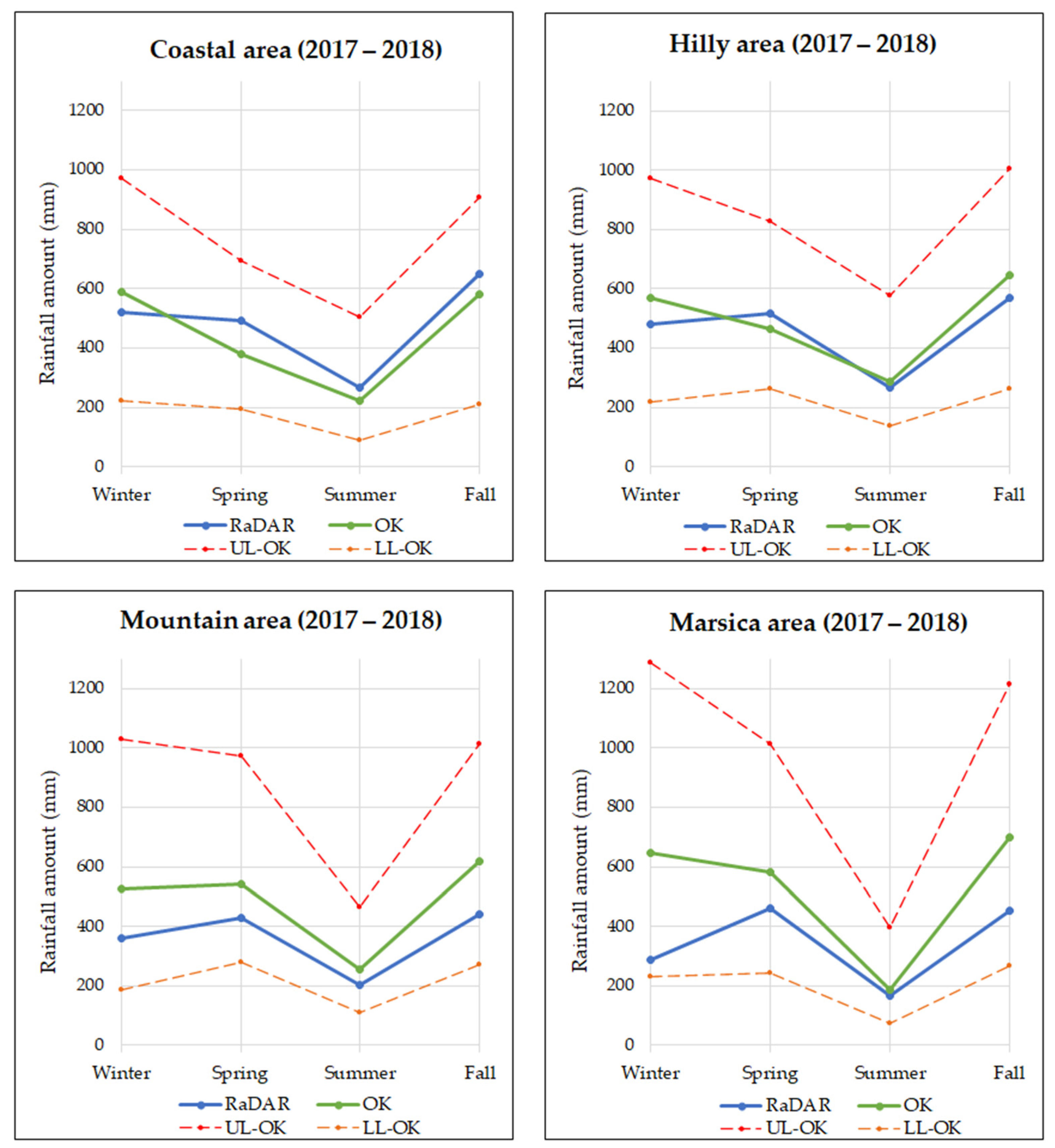
• January, February, and December as winter;
• March, April, and May as spring;
• June, July, and August as summer;
• September, October, and November as fall.

Using both types of data, i.e., weather radar and OK data, monthly rainfall amounts were summed to obtain the quantities reported in Figure 5, where seasonal results are shown for the 2 years analyzed.

As can be seen, all graphs showed higher values in OK interpolated data (OK in the graphs), except for coastal and hilly areas, in which radar and OK tended to a better overall agreement. This can be explained by the fact that those areas were mainly covered by the Il Monte radar, which had the advantage of polarimetry and was positioned closer to sea level, thus, having a closer agreement with ground stations.

The highest discrepancies were shown for winter and fall rainfall amounts, especially in mountain and Marsica areas, whereas the best correspondence was obtained for summer data in all four zones. One possible explanation for this behavior can be attributed to the fact that, in the summer, the freezing-level altitude was higher than in the winter, and consequently, in the summer, radar observations were performed in a rain regime (i.e., they were likely picked up at altitudes below the freezing level). Contrarily, in the winter, the radar more likely sampled in ice/snow regimes, especially when the freezing level approached the radar site altitude (i.e., 1660 m). Thus, as evidenced in Figure 5, in the summer, we expected an augmented consistency between the radar estimations and rain gauges, as the two sources both sampled rain. In this context, the Mt. Midia radar positioned at 1660 m of altitude was disadvantaged during the winter, thus, contributing significantly to the errors registered in the mountain and Marsica areas during the fall and winter periods.

Moreover, the interpolated maps showed a good agreement with the literature data [35] which considered a 79 year period.

As highlighted in Figure 5, the mountain and Marsica zones showed the greatest differences in the seasonal comparison; at the same time, these two were the poorest in terms of rain gauge stations, and weather radar could represent a good solution. For these reasons and for a deeper investigation, rainfall data and the altitudes corresponding to the gauge station locations were correlated.

In any case, the seasonal rainfall amount estimated from RaDAR data always fell into the 95% confidence interval of the OK estimates, which means that they were able to catch the spatial and temporal variability in an acceptable way, and little effort (e.g., bias correction in the postprocessing phase) was required to make them reliable for quantitative purposes.

The OK estimation uncertainty highlights that spatial interpolations obtained using rainfall point measurements can have a low reliability; indeed, they suffer from such a low-density rain gauge monitoring network, as can be seen for the mountain and Fucino areas (Figure 5). As a matter of fact, albeit more accurate at rain gauges, sparse rainfall measurements were not able to catch the spatial variability properly, especially in areas where topography was strongly heterogeneous.

Figure 6 presents this relationship for the 2-year period considered. Rainfall data were from gauge stations located in mountain and Marsica areas and cumulated annually; weather radar data were extracted from annual raster maps at the locations corresponding to the positions of the rain gauge stations within each area considered. Both these rainfall datasets were correlated with automatic station altitudes.

As can be seen, data from gauging stations were more “scattered” than weather radar data, especially in the Marsica area; consequently, these dispersed distributions did not allow deduction of a clear rainfall–altitude correlation.

Despite these issues, both linear and logarithmic regressions were attempted, revealing that the linear correlation fit better than the logarithmic one.

These diagrams confirmed the higher values in the gauge station datasets as already seen in Figure 5; more importantly, they come up with a way to correct radar estimates in complex orography or wide areas [21]. Indeed, the differences (bias) that characterize the two curves (dotted blue and green curves) in Figure 6, which are almost parallel to each other, seemingly suggest that the bias found at a lower altitude is applicable to that at a higher altitude. This finding could be a first step for radar estimate bias correction in pre-selected complex orography environments, i.e., datasets collected in denser areas at lower altitudes can be used to extrapolate the bias found at higher-altitude and less-instrumented areas. Notably, if subseasonal cumulation periods are considered, a different result can be obtained. However, the hydrological application to which such a bias correction can significantly contribute consists of rain infiltration into aquifers, which is more sensitive to seasonal trends of precipitation.

4. Conclusions

Although weather radars are widely used as ground reference in many hydro-meteorological applications, the elaborations performed in this study, verified by their rain estimates, especially in an operational context, can suffer from non-negligible errors if compared with rain gauge networks. Thus, rain gauges and weather radars appear to be integrative with each other; in particular, the former can cooperate with the latter to compensate, at least on average, for some retrieval biases. In that sense, in the future, it will be necessary to develop methods to optimally combine weather radar and rain gauge data in an operational setup. The radar and rain gauge comparison performed in the Abruzzo region highlighted the following positive aspects:

• Good agreement between the two sources in the warmer seasons due to the homogeneity in the quantity observed by the radar and rain gauges;
• Generally good agreement in the coastal and hilly areas due to the better radar coverage in those areas by one of the two radars used in the analysis. This also suggests the importance of studying the radar view geometry compared to the local orography to identify areas where better results are expected.

Among the problematic aspects that require further study, we highlight the following:

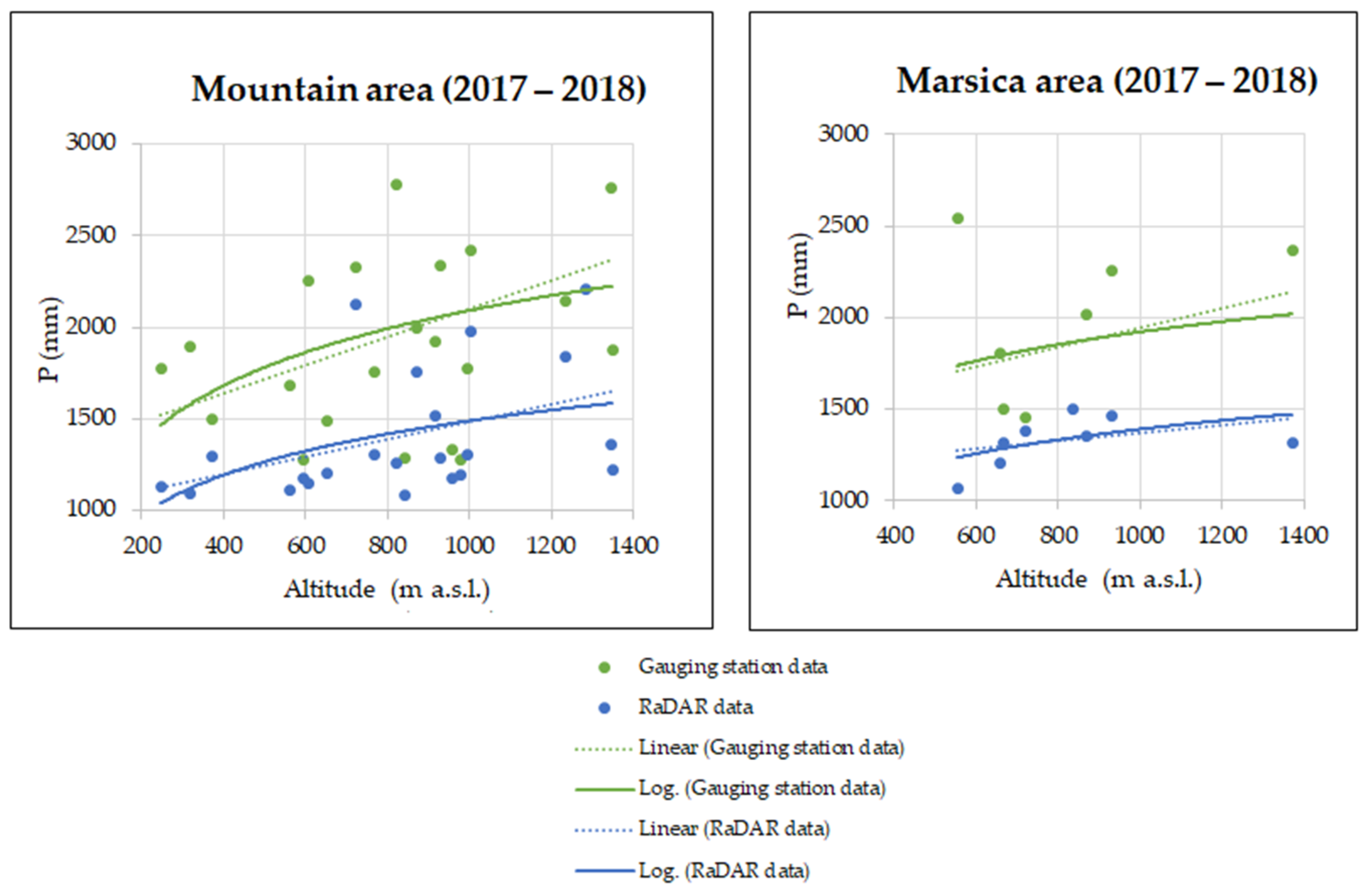
• General underestimation of the results obtained by weather radar. Although the radar underestimation is very well known, its compensation can be less obvious in complex orography, as pointed out in this work. The selection of homogenous climatic and altitude areas, as suggested in this study, could be a way to compensate for the radar underestimation problem,
• Worse agreement between the radar and rain gauges in the cold and rainy seasons (especially in winter and autumn in the mountain and high plain areas), which is justified by the mismatch in the observation of the same precipitation regime by the radar and rain gauge. Such a problem is more severe when the altitude of the radar site is closer to the altitude of the freezing level, because, in such a situation, the radar likely observes ice/snow, whereas rain gauges catch liquid water.

Considering the discrepancies in the results obtained with the two measuring methods, weather radar needs to be better elaborated, compensating for biases in order to fill the lack of directly measured inflows at a high altitude where gauging stations are not present. To this end, future studies will investigate the possibility of using the knowledge of hydrogeological balance in well-known aquifer and catchment areas where the hydrometeor inflow can also be calculated by the sum of the water outlets and evapotranspiration.

References

1. Chiaudani, A.; Di Curzio, D.; Rusi, S. The snow and rainfall impact on the Verde spring behavior: A statistical approach on hydrodynamic and hydrochemical daily time-series. Sci. Total Environ. 2019, 689, 481–493. [Google Scholar] [CrossRef] [PubMed]
2. Fronzi, D.; Di Curzio, D.; Rusi, S.; Valigi, D.; Tazioli, A. Comparison between periodic tracer tests and time-series analysis to assess mid-and long-term recharge model changes due to multiple strong seismic events in carbonate aquifers. Water 2020, 12, 3073. [Google Scholar] [CrossRef]
3. Navarro, A.; García-Ortega, E.; Merino, A.; Sánchez, J.L.; Tapiador, F.J. Orographic biases in IMERG precipitation estimates in the Ebro River basin (Spain): The effects of rain gauge density and altitude. Atm. Res. 2020, 244, 105068. [Google Scholar] [CrossRef]
4. Di Curzio, D.; Rusi, S.; Di Giovanni, A.; Ferretti, E. Evaluation of Groundwater Resources in Minor Plio-Pleistocene Arenaceous Aquifers in Central Italy. Hydrology 2021, 8, 121. [Google Scholar] [CrossRef]
5. Thiessen, A.J.; Alter, C. Precipitation average for large areas. Montly Weather Rev. 1911, 9, 1082–1084. [Google Scholar] [CrossRef]
6. Lyra, G.B.; Correia, T.P.; de Oliveira-Júnior, J.F.; Zeri, M. Evaluation of methods of spatial interpolation for monthly rainfall data over the state of Rio de Janeiro, Brazil. App. Clim. 2018, 134, 955–965. [Google Scholar] [CrossRef]
7. Matheron, G. The intrinsic random functions and their applications. Adv. Appl. Prob. 1973, 5, 439–468. [Google Scholar] [CrossRef] [Green Version]
8. Journel, A.G. Fundamentals of Geostatistics in Five Lessons (Vol. 8); American Geophysical Union: Washington, DC, USA, 1989. [Google Scholar] [CrossRef]
9. Webster, R.; Oliver, M.A. Geostatistics for Environmental Scientists; John Wiley & Sons: New York, NY, USA, 2007. [Google Scholar] [CrossRef] [Green Version]
10. Chilès, J.-P.; Delfiner, P. Geostatistics: Modeling Spatial Uncertainty, 2nd ed.; Wiley: Hoboken, NJ, USA, 2012. [Google Scholar]
11. Castrignanò, A. Introduction to Spatial Data Processing; Aracne: Rome, Italy, 2011. [Google Scholar]
12. Cressie, N. Statistics for Spatial Data; John Wiley & Sons: Hoboken, USA, 2015. [Google Scholar]
13. Barbieri, S.; Di Fabio, S.; Lidori, R.; Rossi, F.L.; Marzano, F.S.; Picciotti, E. Mosaicking Weather Radar Retrievals from an Operational Heterogeneous Network at C and X Band for Precipitation Monitoring in Italian Central Apennines. Rem. Sens. 2022, 14, 248. [Google Scholar] [CrossRef]
14. Falconi, M.T.; Marzano, F.S. Weather Radar Data Processing and Atmospheric Applications: An overview of tools for monitoring clouds and detecting wind shear. IEEE Sig. Proc. Mag. 2019, 36, 85–97. [Google Scholar] [CrossRef]
15. Montopoli, M.; Roberto, N.; Adirosi, E.; Gorgucci, E.; Baldini, L. Investigation of Weather Radar Quantitative Precipitation Estimation Methodologies in Complex Orography. Atmosphere 2017, 8, 34. [Google Scholar] [CrossRef] [Green Version]
16. Germann, U.; Boscacci, M.; Clementi, L.; Gabella, M.; Hering, A.; Sartori, M.; Sideris, I.V.; Calpini, B. Weather Radar in Complex Orography. Rem. Sens. 2022, 14, 503. [Google Scholar] [CrossRef]
17. Vulpiani, G.; Montopoli, M.; Delli Passeri, L.; Gioia, A.G.; Giordano, P.; Marzano, F.S. On the use of dual-polarized C-band RaDAR for operational rainfall retrieval in mountainous areas. J. Appl. Meteor. Climat. 2012, 51, 405–425. [Google Scholar] [CrossRef]
18. Federico, S.; Torcasio, R.C.; Avolio, E.; Caumont, O.; Montopoli, M.; Baldini, L.; Vulpiani, G.; Dietrich, S. The impact of lightning and radar reflectivity factor data assimilation on the very short-term rainfall forecasts of RAMS@ISAC: Application to two case studies in Italy. Nat. Haz. Ear. Syst. Sci. 2019, 19, 1839–1864. [Google Scholar] [CrossRef] [Green Version]
19. Montopoli, M.; Picciotti, E.; Baldini, L.; Di Fabio, S.; Marzano, F.S.; Vulpiani, G. Gazing inside a giant-hail-bearing Mediterranean supercell by dual-polarization Doppler weather RaDAR. Atm. Res. 2021, 264, 105852. [Google Scholar] [CrossRef]
20. Di Curzio, D.; Di Giovanni, A.; Lidori, R.; Marzano, F.S.; Rusi, S. Investigating the feasibility of using precipitation measurements from weather RaDAR to estimate potential recharge in regional aquifers: The Majella massif case study in Central Italy. Acq. Sott.-Ital. J. Groun. 2022, 11, 41–51. [Google Scholar] [CrossRef]
21. Areerachakul, N.; Prongnuch, S.; Longsomboon, P.; Kandasamy, J. Quantitative Precipitation Estimation (QPE) Rainfall from Meteorology Radar over Chi Basin. Hydrology 2022, 9, 178. [Google Scholar] [CrossRef]
22. Sollitto, D.; Romic, M.; Castrignanò, A.; Romic, D.; Bakic, H. Assessing heavy metal contamination in soils of the Zagreb region (Northwest Croatia) using multivariate geostatistics. Catena 2010, 80, 182–194. [Google Scholar] [CrossRef]
23. Di Curzio, D.; Rusi, S.; Signanini, P. Advanced redox zonation of the San Pedro Sula alluvial aquifer (Honduras) using data fusion and multivariate geostatistics. Sci. Total Environ. 2019, 695, 133796. [Google Scholar] [CrossRef]
24. Manzione, R.L.; Castrignanò, A. A geostatistical approach for multi-source data fusion to predict water table depth. Sci. Total Environ. 2019, 696, 133763. [Google Scholar] [CrossRef]
25. Vessia, G.; Di Curzio, D.; Chiaudani, A.; Rusi, S. Regional rainfall threshold maps drawn through multivariate geostatistical techniques for shallow landslide hazard zonation. Sci. Total Environ. 2020, 705, 135815. [Google Scholar] [CrossRef]
26. Rivoirard, J. On the structural link between variables in kriging with external drift. Math. Geol. 2002, 34, 797–808. [Google Scholar] [CrossRef]
27. Hengl, T.; Geuvelink, G.B.M.; Stein, A. Comparison of Kriging with External Drift and Regression-Kriging. Technical Note, ITC, The Netherlands. 2003. Available online: http://www.itc.nl/library/Academic.output (accessed on 1 October 2022).
28. Buttafuoco, G.; Conforti, M. Improving Mean Annual Precipitation Prediction Incorporating Elevation and Taking into Account Support Size. Water 2021, 13, 830. [Google Scholar] [CrossRef]
29. Vergni, L.; Di Lena, B.; Chiaudani, A. Statistical characterisation of winter precipitation in the Abruzzo region (Italy) in relation to the North Atlantic Oscillation (NAO). Atmos. Res. 2016, 178–179, 279–290. [Google Scholar] [CrossRef]
30. Vergni, L.; Todisco, F.; Di Lena, B.; Mannocchi, F. Effect of the North Atlantic Oscillation on winter daily rainfall and runoff in the Abruzzo region (Central Italy). Stoch Env. Res. Risk Assess. 2016, 30, 1901–1915. [Google Scholar] [CrossRef]
31. Vessia, G.; Di Curzio, D.; Castrignanò, A. Modeling 3D soil lithotypes variability through geostatistical data fusion of CPT parameters. Sci. Total Environ. 2020, 698, 134340. [Google Scholar] [CrossRef] [PubMed]
32. Goovaerts, P. Geostatistics for Natural Resources Evaluation; Oxford University Press: Oxford, UK, 1997. [Google Scholar]
33. Adirosi, E.; Roberto, N.; Montopoli, M.; Gorgucci, E.; Baldini, L. Influence of Disdrometer Type on Weather Radar Algorithms from Measured DSD: Application to Italian Climatology. Atmosphere 2018, 9, 360. [Google Scholar] [CrossRef] [Green Version]
34. Harrison, D.L.; Driscoll, S.J.; Kitchen, M. Improving precipitation estimates from weather radar using quality control and correction techniques. Meteorol. Appl. 2000, 7, 135–144. [Google Scholar] [CrossRef] [Green Version]
35. Curci, G.; Guijarro, J.A.; Di Antonio, L.; Di Bacco, M.; Di Lena, B.; Scorzini, A.R. Building a local climate reference dataset: Application to the Abruzzo region (Central Italy), 1930–2019. Int. J. Climatol. 2021, 41, 4414–4436. [Google Scholar] [CrossRef]
Figure 1. Study area divided in the four zones. Rain gauge and radar sensors are shown.
Hydrology 09 00225 g001
Figure 2. Raster map showing the radar monthly cumulate for March 2017. Altimetric/climatic zones are also displayed.
Hydrology 09 00225 g002
Figure 3. Variogram (variance vs. distance) examples. To the left: 2017; to the right: 2018. The numbers on the variogram curves indicate the number of pairs.
Hydrology 09 00225 g003
Figure 4. Comparison between OK interpolated data and weather radar ones using the raster maps sliced in the four zones: (a) 2017 OK interpolated data; (b) 2017 weather radar data; (c) 2018 OK interpolated data; (d) 2018 weather radar data.
Hydrology 09 00225 g004
Figure 5. Rainfall amount (mm) for each altimetric area considering seasonal datasets for both radar and OK interpolated data (OK); upper limits (UL-OK) and lower limits (LL-OK) of the confidence intervals are also shown.
Hydrology 09 00225 g005
Figure 6. Correlation altitude/precipitation (P) using rainfall data from gauging stations and weather radar datasets in mountain and Marsica areas for 2017–2018 years. Linear and Log. indicate regression lines.
Hydrology 09 00225 g006