
Exploration of the Advanced VIVOTM Joint Simulator: An In-Depth Analysis of Opportunities and Limitations Demonstrated by the Artificial Knee Joint


Abstract
:
1. Introduction
2. Materials and Methods
2.1. Six Degrees of Freedom Joint Simulator VIVOTM
2.1.1. Physical Setup
2.1.2. Definition of Coordinate Systems
2.1.3. Force and Moment Interpretation
2.1.4. Controller Design
2.2. Experimental Configuration for Testing of Total Knee Endoprostheses
Functional Principle
2.3. Parameter Variations for Sensitivity Analysis
2.3.1. Influence of Control Method
2.3.2. Repeatability and Kinematic Reproducibility
2.3.3. Effect of the Flexible Bellows
2.3.4. Effect of the Waveform Frequency
2.3.5. Effect of Lubrication
2.3.6. Sensitivity to Embedding of the Implant Components
3. Results
3.1. Influence of Control Method
3.1.1. Comparison of ILC and PI Mode
3.1.2. Occurrence of Oscillation
3.2. Repeatability and Kinematic Reproducibility
3.3. Effect of the Flexible Bellows
3.4. Effect of the Waveform Frequency
3.5. Effect of Lubrication
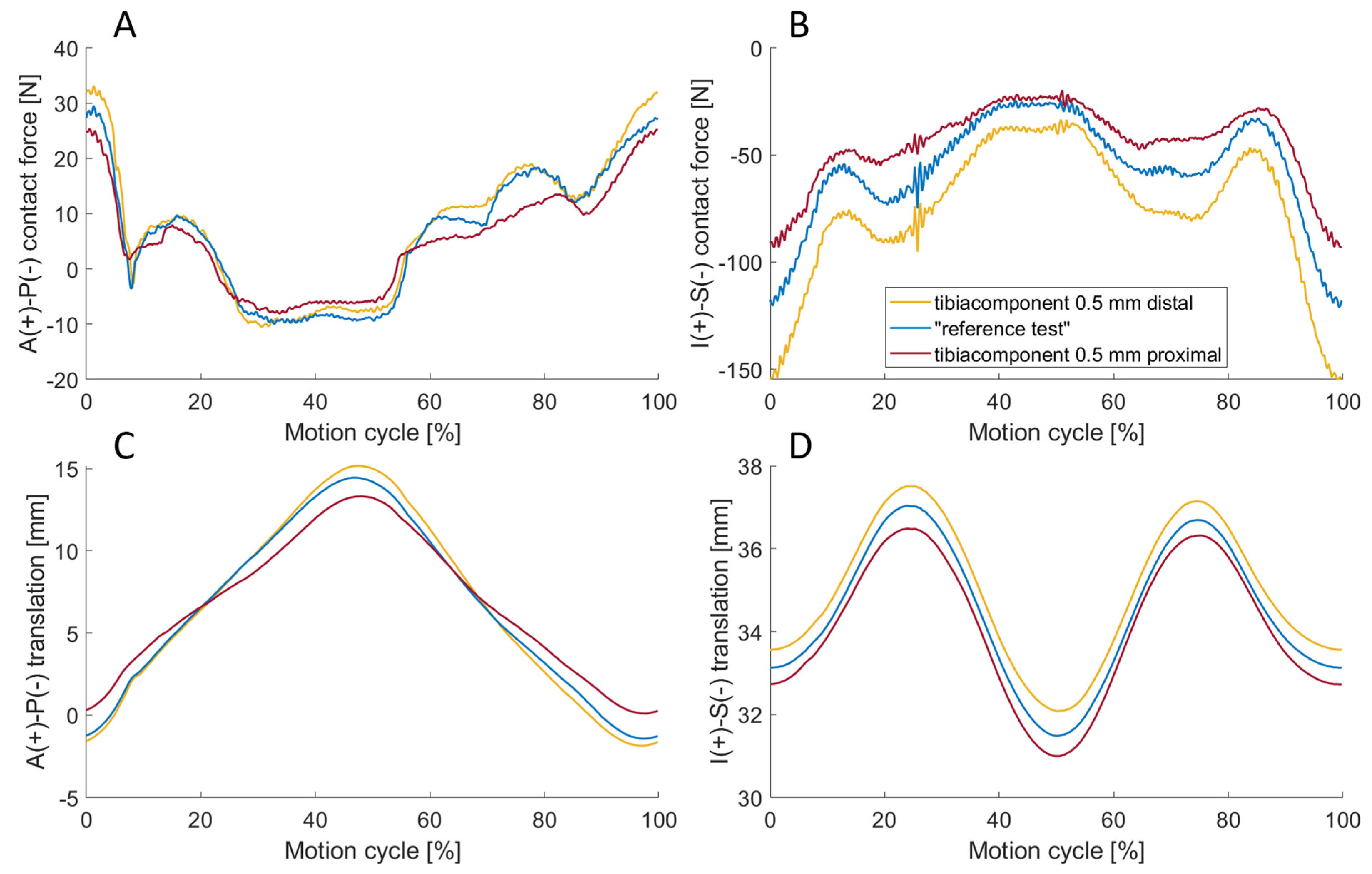
3.6. Sensitivity to Embedding of the Implant Components
4. Discussion
4.1. Influence of Control Method
4.2. Repeatability and Kinematic Reproducibility
4.3. Effect of the Flexible Bellows
4.4. Effect of the Waveform Frequency
4.5. Effect of Lubrication
4.6. Sensitivity to Embedding of the Implant Components
4.7. Limitations
5. Conclusions
Author Contributions
Funding
Institutional Review Board Statement
Informed Consent Statement
Data Availability Statement
Acknowledgments
Conflicts of Interest
Appendix A

| Force | Displacement | ||||
|---|---|---|---|---|---|
| Control Parameters | Integral Gain (mm/s)/N | Proportional Gain mm/N | Maximum Rate (mm/s) | Integral Gain (mm/s)/mm | Servo Bandwidth |
| ML | 0.02 | 0.003 | 10 | 5 | 6 |
| AP | 0.02 | 0.003 | 10 | 5 | 6 |
| VL | 0.1 | 0.005 | 10 | 5 | 6 |
| (deg/s) | |||||
| FL | 10 | 0.2 | 0.2 | 20 | 5 |
| Abd | 10 | 0.2 | 0.2 | 20 | 6 |
| IE | 10 | 0.2 | 0.2 | 20 | 6 |
| Force | Displacement | ||||
|---|---|---|---|---|---|
| Control Parameters | Integral Gain (mm/s)/N | Proportional Gain mm/N | Maximum Rate (mm/s) | Integral Gain (mm/s)/mm | Servo Bandwidth |
| ML | 0.02 | 0.003 | 10 | 5 | 6 |
| AP | 0.02 | 0.003 | 10 | 5 | 6 |
| VL | 0.1 | 0.02 | 15 | 5 | 6 |
| (deg/s) | |||||
| FL | 10 | 0.2 | 0.2 | 20 | 5 |
| Abd | 10 | 0.2 | 0.2 | 20 | 6 |
| IE | 10 | 0.2 | 0.2 | 20 | 6 |
References
- Blankevoort, L.; Huiskes, R. Ligament-bone interaction in a three-dimensional model of the knee. J. Biomech. Eng. 1991, 113, 263–269. [Google Scholar] [CrossRef]
- Walker, P.S.; Blunn, G.W.; Lilley, P.A. Wear testing of materials and surfaces for total knee replacement. J. Biomed. Mater. Res. 1996, 33, 159–175. [Google Scholar] [CrossRef]
- ISO 14242-1:2014-10; Implants for Surgery—Wear of Total Hip-Joint Prostheses—Part 1: Loading and Displacement Parameters for Wear-Testing Machines and Corresponding Environmental Conditions for Test. ISO International Organization for Standardization, Beuth Verlag GmbH: Berlin, Germany, 2014.
- ISO 14243-1:2009-11; Implants for Surgery—Wear of Total Knee-Joint Prostheses—Part 1: Loading and Displacement Parameters for Wear-Testing Machines with Load Control and Corresponding Environmental Conditions for Test. ISO International Organization for Standardization, Beuth Verlag GmbH: Berlin, Germany, 2009.
- Bergmann, G.; Bender, A.; Graichen, F.; Dymke, J.; Rohlmann, A.; Trepczynski, A.; Heller, M.O.; Kutzner, I. Standardized loads acting in knee implants. PLoS ONE 2014, 9, e86035. [Google Scholar] [CrossRef]
- Abdelgaied, A.; Fisher, J.; Jennings, L.M. Understanding the differences in wear testing method standards for total knee replacement. J. Mech. Behav. Biomed. Mater. 2022, 132, 105258. [Google Scholar] [CrossRef] [PubMed]
- Rychlik, M.; Wendland, G.; Jackowski, M.; Rennert, R.; Schaser, K.-D.; Nowotny, J. Calibration procedure and biomechanical validation of an universal six degree-of-freedom robotic system for hip joint testing. J. Orthop. Surg. Res. 2023, 18, 164. [Google Scholar] [CrossRef] [PubMed]
- Marra, M.A.; Strzelczak, M.; Heesterbeek, P.J.C.; van de Groes, S.A.W.; Janssen, D.; Koopman, B.F.J.M.; Verdonschot, N.; Wymenga, A.B. Flexing and downsizing the femoral component is not detrimental to patellofemoral biomechanics in posterior-referencing cruciate-retaining total knee arthroplasty. Knee Surg. Sports Traumatol. Arthrosc. 2018, 26, 3377–3385. [Google Scholar] [CrossRef] [PubMed]
- Tischer, T.; Geier, A.; Lutter, C.; Enz, A.; Bader, R.; Kebbach, M. Patella height influences patellofemoral contact and kinematics following cruciate-retaining total knee replacement. J. Orthop. Res. 2023, 41, 793–802. [Google Scholar] [CrossRef] [PubMed]
- Kebbach, M.; Geier, A.; Darowski, M.; Krueger, S.; Schilling, C.; Grupp, T.M.; Bader, R. Computer-based analysis of different component positions and insert thicknesses on tibio-femoral and patello-femoral joint dynamics after cruciate-retaining total knee replacement. Knee 2023, 40, 152–165. [Google Scholar] [CrossRef] [PubMed]
- Khasian, M.; Meccia, B.A.; LaCour, M.T.; Komistek, R.D. Effects of Posterior Tibial Slope on a Posterior Cruciate Retaining Total Knee Arthroplasty Kinematics and Kinetics. J. Arthroplast. 2021, 36, 2379–2385. [Google Scholar] [CrossRef] [PubMed]
- Tzanetis, P.; Fluit, R.; Souza, K.D.; Robertson, S.; Koopman, B.; Verdonschot, N. Pre-Planning the Surgical Target for Optimal Implant Positioning in Robotic-Assisted Total Knee Arthroplasty. Bioengineering 2023, 10, 543. [Google Scholar] [CrossRef] [PubMed]
- Putame, G.; Terzini, M.; Rivera, F.; Kebbach, M.; Bader, R.; Bignardi, C. Kinematics and kinetics comparison of ultra-congruent versus medial-pivot designs for total knee arthroplasty by multibody analysis. Sci. Rep. 2022, 12, 3052. [Google Scholar] [CrossRef]
- Kebbach, M.; Grawe, R.; Geier, A.; Winter, E.; Bergschmidt, P.; Kluess, D.; D’Lima, D.; Woernle, C.; Bader, R. Effect of surgical parameters on the biomechanical behaviour of bicondylar total knee endoprostheses—A robot-assisted test method based on a musculoskeletal model. Sci. Rep. 2019, 9, 14504. [Google Scholar] [CrossRef]
- AMTI Force and Motion. VivoControl Software Technical Reference Manual: Version 1.0.0; Advanced Mechanical Technology Inc.: Watertown, MA, USA, 2015. [Google Scholar]
- Sharifi Kia, D.; Willing, R. Applying a Hybrid Experimental-Computational Technique to Study Elbow Joint Ligamentous Stabilizers. J. Biomech. Eng. 2018, 140, 061012. [Google Scholar] [CrossRef]
- Willing, R. Comparing damage on retrieved total elbow replacement bushings with lab worn specimens subjected to varied loading conditions. J. Orthop. Res. 2018, 36, 1998–2006. [Google Scholar] [CrossRef]
- Navacchia, A.; Clary, C.W.; Han, X.; Shelburne, K.B.; Wright, A.P.; Rullkoetter, P.J. Loading and kinematic profiles for patellofemoral durability testing. J. Mech. Behav. Biomed. Mater. 2018, 86, 305–313. [Google Scholar] [CrossRef]
- Behnam, Y.A.; Anantha Krishnan, A.; Wilson, H.; Clary, C.W. Simultaneous Evaluation of Tibiofemoral and Patellofemoral Mechanics in Total Knee Arthroplasty: A Combined Experimental and Computational Approach. J. Biomech. Eng. 2024, 146, 011007. [Google Scholar] [CrossRef] [PubMed]
- Fitzpatrick, C.K.; Maag, C.; Clary, C.W.; Metcalfe, A.; Langhorn, J.; Rullkoetter, P.J. Validation of a new computational 6-DOF knee simulator during dynamic activities. J. Biomech. 2016, 49, 3177–3184. [Google Scholar] [CrossRef]
- Sekeitto, A.R.; McGale, J.G.; Montgomery, L.A.; Vasarhelyi, E.M.; Willing, R.; Lanting, B.A. Posterior-stabilized total knee arthroplasty kinematics and joint laxity: A hybrid biomechanical study. Arthroplasty 2022, 4, 53. [Google Scholar] [CrossRef]
- Maag, C.; Cracaoanu, I.; Langhorn, J.; Heldreth, M. Total knee replacement wear during simulated gait with mechanical and anatomic alignments. Proc. Inst. Mech. Eng. H 2021, 235, 515–522. [Google Scholar] [CrossRef] [PubMed]
- Montgomery, L.; Willing, R.; Lanting, B. Virtual Joint Motion Simulator Accurately Predicts Effects of Femoral Component Malalignment during TKA. Bioengineering 2023, 10, 503. [Google Scholar] [CrossRef] [PubMed]
- Cuevas-Andrade, J.L.; Beltrán-Fernández, J.A.; Hermida-Ochoa, J.C.; Rebattú y González, M.G.; Hernández-Gómez, L.H.; Uribe-Cortés, T.B.; Trujillo-Pérez, C.A.; Moreno-Garibaldi, P. Dynamic and Experimental Testing of a Biomechanical System: Cadaveric Temporomandibular Specimen and a Multiaxial Joint. In Engineering Design Applications V; Öchsner, A., Altenbach, H., Eds.; Springer Nature Switzerland: Cham, Switzerland, 2023; pp. 251–280. ISBN 978-3-031-26465-8. [Google Scholar]
- Baldwin, M.A.; Clary, C.W.; Fitzpatrick, C.K.; Deacy, J.S.; Maletsky, L.P.; Rullkoetter, P.J. Dynamic finite element knee simulation for evaluation of knee replacement mechanics. J. Biomech. 2012, 45, 474–483. [Google Scholar] [CrossRef]
- Bahçe, E.; Emir, E. Investigation of wear of ultra high molecular weight polyethylene in a soft tissue behaviour knee joint prosthesis wear test simulator. J. Mater. Res. Technol. 2019, 8, 4642–4650. [Google Scholar] [CrossRef]
- Bortel, E.; Charbonnier, B.; Heuberger, R. Development of a Synthetic Synovial Fluid for Tribological Testing. Lubricants 2015, 3, 664–686. [Google Scholar] [CrossRef]
- Brandt, J.-M.; Charron, K.D.; Zhao, L.; MacDonald, S.J.; Medley, J.B. Lubricant Biochemistry Affects Polyethylene Wear in Knee Simulator Testing. Biotribology 2021, 27, 100185. [Google Scholar] [CrossRef]
- Nečas, D.; Usami, H.; Niimi, T.; Sawae, Y.; Křupka, I.; Hartl, M. Running-in friction of hip joint replacements can be significantly reduced: The effect of surface-textured acetabular cup. Friction 2020, 8, 1137–1152. [Google Scholar] [CrossRef]
- Herrmann, S.; Kluess, D.; Kaehler, M.; Grawe, R.; Rachholz, R.; Souffrant, R.; Zierath, J.; Bader, R.; Woernle, C. A Novel Approach for Dynamic Testing of Total Hip Dislocation under Physiological Conditions. PLoS ONE 2015, 10, e0145798. [Google Scholar] [CrossRef] [PubMed]
- Wismans, J.; Veldpaus, F.; Janssen, J.; Huson, A.; Struben, P. A three-dimensional mathematical model of the knee-joint. J. Biomech. 1980, 13, 677–685. [Google Scholar] [CrossRef] [PubMed]
- Blankevoort, L.; Kuiper, J.H.; Huiskes, R.; Grootenboer, H.J. Articular contact in a three-dimensional model of the knee. J. Biomech. 1991, 24, 1019–1031. [Google Scholar] [CrossRef] [PubMed]
- Grood, E.S.; Suntay, W.J. A joint coordinate system for the clinical description of three-dimensional motions: Application to the knee. J. Biomech. Eng. 1983, 105, 136–144. [Google Scholar] [CrossRef]
- Kebbach, M.; Darowski, M.; Krueger, S.; Schilling, C.; Grupp, T.M.; Bader, R.; Geier, A. Musculoskeletal Multibody Simulation Analysis on the Impact of Patellar Component Design and Positioning on Joint Dynamics after Unconstrained Total Knee Arthroplasty. Materials 2020, 13, 2365. [Google Scholar] [CrossRef]
- Dreyer, M.J.; Trepczynski, A.; Hosseini Nasab, S.H.; Kutzner, I.; Schütz, P.; Weisse, B.; Dymke, J.; Postolka, B.; Moewis, P.; Bergmann, G.; et al. European Society of Biomechanics S.M. Perren Award 2022: Standardized tibio-femoral implant loads and kinematics. J. Biomech. 2022, 141, 111171. [Google Scholar] [CrossRef] [PubMed]
- MacWilliams, B.A.; Davis, R.B. Addressing some misperceptions of the joint coordinate system. J. Biomech. Eng. 2013, 135, 54506. [Google Scholar] [CrossRef] [PubMed]
- Walker, P.S.; Mhadgut, A.; Buchalter, D.B.; Kirby, D.J.; Hennessy, D. The effect of total knee geometries on kinematics: An experimental study using a crouching machine. J. Orthop. Res. 2021, 39, 2537–2545. [Google Scholar] [CrossRef] [PubMed]
- Rahnemai-Azar, A.A.; Yoshida, M.; Musahl, V.; Debski, R. In Vitro Biomechanical Analysis of Knee Rotational Stability. In Rotatory Knee Instability; Musahl, V., Karlsson, J., Kuroda, R., Zaffagnini, S., Eds.; Springer International Publishing: Cham, Switzerland, 2017; pp. 3–14. ISBN 978-3-319-32069-4. [Google Scholar]
- Coles, L.G.; Gheduzzi, S.; Miles, A.W. In vitro method for assessing the biomechanics of the patellofemoral joint following total knee arthroplasty. Proc. Inst. Mech. Eng. H 2014, 228, 1217–1226. [Google Scholar] [CrossRef] [PubMed]
- Lowry, M.; Rosenbaum, H.; Walker, P.S. Evaluation of total knee mechanics using a crouching simulator with a synthetic knee substitute. Proc. Inst. Mech. Eng. H 2016, 230, 421–428. [Google Scholar] [CrossRef] [PubMed]
- Bristow, D.A.; Tharayil, M.; Alleyne, A.G. A survey of iterative learning control. IEEE Control Syst. 2006, 26, 96–114. [Google Scholar] [CrossRef]
- Hosseini Nasab, S.H.; List, R.; Oberhofer, K.; Fucentese, S.F.; Snedeker, J.G.; Taylor, W.R. Loading Patterns of the Posterior Cruciate Ligament in the Healthy Knee: A Systematic Review. PLoS ONE 2016, 11, e0167106. [Google Scholar] [CrossRef]
- Bobrowitsch, E.; Lorenz, A.; Wülker, N.; Walter, C. Simulation of in vivo dynamics during robot assisted joint movement. Biomed. Eng. Online 2014, 13, 167. [Google Scholar] [CrossRef]
- Pfitzner, T.; Moewis, P.; Stein, P.; Boeth, H.; Trepczynski, A.; Roth, P.V.; Duda, G.N. Modifications of femoral component design in multi-radius total knee arthroplasty lead to higher lateral posterior femoro-tibial translation. Knee Surg. Sports Traumatol. Arthrosc. 2018, 26, 1645–1655. [Google Scholar] [CrossRef]
- Bracey, D.N.; Brown, M.L.; Beard, H.R.; Mannava, S.; Nazir, O.F.; Seyler, T.M.; Lang, J.E. Effects of patellofemoral overstuffing on knee flexion and patellar kinematics following total knee arthroplasty: A cadaveric study. Int. Orthop. 2015, 39, 1715–1722. [Google Scholar] [CrossRef]
- Ziegler, J.G.; Nichols, N.B. Optimum Settings for Automatic Controllers. J. Dyn. Syst. Meas. Control 1993, 115, 220–222. [Google Scholar] [CrossRef]
- Jay, G.D.; Waller, K.A. The biology of lubricin: Near frictionless joint motion. Matrix Biol. 2014, 39, 17–24. [Google Scholar] [CrossRef] [PubMed]


| Name | Stiffness [N] | Reference Strain [%] |
|---|---|---|
| aPCL | 3000 | −11.373 |
| pPCL | 1500 | −7.552 |
| aMCL | 1500 | 4.321 |
| pMCL | 1500 | 4.298 |
| dMCL | 1500 | −2.783 |
| aLCL | 1800 | 5.741 |
| pLCL | 2250 | 3.912 |
| pOPL | 1250 | 5.826 |
| dOPL | 1250 | 5.891 |
| APL | 1500 | −1.642 |
| lpCAP | 2500 | −1.167 |
| mpCAP | 2500 | −2.366 |
| RMSE | L-M Force Tracking Error [N] | A-P Force Tracking Error [N] | I-S Force Tracking Error [N] | F-E Angle Tracking Error [°] | A-A Moment Tracking Error [Nm] | E-I Moment Tracking Error [Nm] |
|---|---|---|---|---|---|---|
| PI cycle 2–7 | 13.0 | 67.0 | 52.3 | 2.54 | 1.2 | 0.6 |
| ILC cycle 2–7 | 14.0 | 51.3 | 196.9 | 8.26 | 2.4 | 0.5 |
| ILC cycle 96–100 | 2.1 | 19.9 | 6.7 | 0.04 | 0.6 | 0.3 |
| ILC cycle 196–200 | 1.5 | 13.3 | 5.2 | 0.04 | 0.4 | 0.3 |
| ILC cycle 296–300 | 1.6 | 10.1 | 5.2 | 0.04 | 0.3 | 0.3 |
| RMSE of the I-S Tracking Error [N] | Cycle 2 | Cycle 49 | Cycle 300 |
|---|---|---|---|
| ILC “reference test” | 506.5 | 11.1 | 5.2 |
| ILC adapted values | 81.2 | 39.3 | - |
| Pi control | 51.6 | 52.2 | - |
| RMSE of the Tracking Error | L-M Translation Tracking Error [mm] | A-P Translation Tracking Error [mm] | I-S Translation Tracking Error [mm] | F-E Angle Tracking Error [°] | A-A Angle Tracking Error [°] | E-I Angle Tracking Error [°] |
|---|---|---|---|---|---|---|
| 0.01 | 0.01 | 0.00 | 0.04 | 0.04 | 0.01 |
| Correlation Factor | L-M Contact Force | A-P Contact Force | I-S Contact Force | F-E Contact Moment | A-A Contact Moment | E-I Contact Moment |
|---|---|---|---|---|---|---|
| Repeatability | 0.98 | 0.99 | 1.00 | 1.00 | 0.96 | 0.93 |
| kinematic reproducibility | 0.99 | 0.99 | 0.98 | 1.00 | 0.99 | 0.99 |
| RMSE of the Tracking Error | L-M Force Tracking Error [N] | A-P Force Tracking Error [N] | I-S Force Tracking Error [N] | F-E Angle Tracking Error [°] | A-A Moment Tracking Error [Nm] | E-I Moment Tracking Error [Nm] |
|---|---|---|---|---|---|---|
| f = 0.1 | 1.7 | 9.8 | 3.9 | 0.01 | 0.3 | 0.2 |
| f = 0.25 | 1.5 | 10.1 | 5.1 | 0.04 | 0.3 | 0.3 |
| f = 0.5 | 1.4 | 10.6 | 5.1 | 0.04 | 0.2 | 0.2 |
| RMSE of the Tracking Error | M-L Force Tracking Error [N] | A-P Force Tracking Error [N] | S-I Force Tracking Error [N] | F-E Angle Tracking Error [°] | A-A Moment Tracking Error [Nm] | I-E Moment Tracking Error [Nm] |
|---|---|---|---|---|---|---|
| lubricated | 0.9 | 6.6 | 4.0 | 0.03 | 0.3 | 0.3 |
| unlubricated (“reference test”) | 1.5 | 10.1 | 5.1 | 0.04 | 0.3 | 0.3 |
Disclaimer/Publisher’s Note: The statements, opinions and data contained in all publications are solely those of the individual author(s) and contributor(s) and not of MDPI and/or the editor(s). MDPI and/or the editor(s) disclaim responsibility for any injury to people or property resulting from any ideas, methods, instructions or products referred to in the content. |
© 2024 by the authors. Licensee MDPI, Basel, Switzerland. This article is an open access article distributed under the terms and conditions of the Creative Commons Attribution (CC BY) license (https://creativecommons.org/licenses/by/4.0/).
Share and Cite
Henke, P.; Ruehrmund, L.; Bader, R.; Kebbach, M. Exploration of the Advanced VIVOTM Joint Simulator: An In-Depth Analysis of Opportunities and Limitations Demonstrated by the Artificial Knee Joint. Bioengineering 2024, 11, 178. https://doi.org/10.3390/bioengineering11020178
Henke P, Ruehrmund L, Bader R, Kebbach M. Exploration of the Advanced VIVOTM Joint Simulator: An In-Depth Analysis of Opportunities and Limitations Demonstrated by the Artificial Knee Joint. Bioengineering. 2024; 11(2):178. https://doi.org/10.3390/bioengineering11020178
Chicago/Turabian StyleHenke, Paul, Leo Ruehrmund, Rainer Bader, and Maeruan Kebbach. 2024. "Exploration of the Advanced VIVOTM Joint Simulator: An In-Depth Analysis of Opportunities and Limitations Demonstrated by the Artificial Knee Joint" Bioengineering 11, no. 2: 178. https://doi.org/10.3390/bioengineering11020178