Article

Grey Wolf Optimizer with Behavior Considerations and Dimensional Learning in Three-Dimensional Tooth Model Reconstruction

by
Ritipong Wongkhuenkaew
1,
Sansanee Auephanwiriyakul
2,*,
Marasri Chaiworawitkul
3,
Nipon Theera-Umpon
4 and
Uklid Yeesarapat
5
1
Department of Computer Engineering, Faculty of Engineering, Biomedical Engineering Institute, Biomedical Engineering and Innovation Research Center, Chiang Mai University, Chiang Mai 50200, Thailand
2
Department of Computer Engineering, Faculty of Engineering, Excellence Center in Infrastructure Technology and Transportation Engineering, Biomedical Engineering Institute, Biomedical Engineering and Innovation Research Center, Chiang Mai University, Chiang Mai 50200, Thailand
3
Orthodontics and Pediatric Dentistry Department, Faculty of Dentistry, Chiang Mai University, Chiang Mai 50200, Thailand
4
Department of Electrical Engineering, Faculty of Engineering, Biomedical Engineering Institute, Biomedical Engineering and Innovation Research Center, Chiang Mai University, Chiang Mai 50200, Thailand
5
Department of Computer Engineering, Faculty of Engineering, Chiang Mai University, Empress Dental Care Clinic, Chiang Mai 50200, Thailand
*
Author to whom correspondence should be addressed.
Bioengineering 2024, 11(3), 254; https://doi.org/10.3390/bioengineering11030254
Submission received: 26 December 2023 / Revised: 25 February 2024 / Accepted: 1 March 2024 / Published: 5 March 2024

Abstract

:
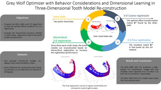
Three-dimensional registration with the affine transform is one of the most important steps in 3D reconstruction. In this paper, the modified grey wolf optimizer with behavior considerations and dimensional learning (BCDL-GWO) algorithm as a registration method is introduced. To refine the 3D registration result, we incorporate the iterative closet point (ICP). The BCDL-GWO with ICP method is implemented on the scanned commercial orthodontic tooth and regular tooth models. Since this is a registration from multi-views of optical images, the hierarchical structure is implemented. According to the results for both models, the proposed algorithm produces high-quality 3D visualization images with the smallest mean squared error of about 7.2186 and 7.3999 μm2, respectively. Our results are compared with the statistical randomization-based particle swarm optimization (SR-PSO). The results show that the BCDL-GWO with ICP is better than those from the SR-PSO. However, the computational complexities of both methods are similar.

Graphical Abstract

1. Introduction

Three-dimensional reconstruction from multi-view images has been used in many applications, including in orthodontics. It is also used in diagnostic and treatment planning processes in adults and children with dental caries [1,2], especially dental caries that are a cause of chronic diseases in children [3]. With recent technology, e.g., laser or CT, there are several 3D reconstructions from multimodal images research works [4,5,6,7,8,9] from those technologies. However, in rural areas, there is limited access to these sophisticated devices and also insufficient oral healthcare [10]. In Thailand, the Dental Innovation Foundation, under royal patronage, has provided dental care access in rural communities for a long time. Due to limited access to sophisticated devices in those communities, taking multi-view teeth images inside children’s mouths is a very difficult task. Hence, multi-view teeth optical images are collected to be utilized in the 3D reconstruction system. In 3D reconstruction from multi-view images, there are several processes, including image registration, which is the transforming process of different sets of data into one coordinate system. There are existing works on 2D medical image registration [11,12,13,14,15,16,17,18,19,20,21,22,23,24,25,26]. Since point cloud coordinates are used in our 3D teeth reconstruction, the 3D registration is more proper. In the literature, there are several works on 3D registration [27,28,29,30,31] utilizing several features in the registration process, including point cloud coordinates representing the 3D shapes of objects [32,33,34,35,36,37]. These mentioned works used a variation swarm optimization (PSO) in the location matching between the source and target images. In the hope of improving the registration accuracy, there was study conducted on using the grey wolf optimizer (GWO) instead of PSO in 3D registration [38]. However, only rotation and/or translation were used in those matching locations. Hence, in our previous work [39], the statistical randomization-based particle swarm optimization (SR-PSO) algorithm with the iterative closet point (ICP) method was used to find the optimal affine transform (translation, scaling, rotation, and shearing (shortened from a shearing mapping that displaces each point in a fixed direction by an amount proportional to its signed distance from a given line parallel to that direction)) between teeth optical images.
In particular, a system with the 3D registration using a modified grey wolf optimizer that can reconstruct a 3D image from teeth optical images is developed. However, due to a research ethical approval requirement, we will not use real images taken from children. Hence, we postulate scanned images from two commercial tooth models and then create point cloud images [39]. To avoid premature convergence and to balance between exploration and exploitation, we modify the grey wolf optimization algorithm [40] with behavior considerations and dimensional learning strategies [41,42,43,44], called BCDL-GWO, to find the suitable affine transform between the source and target images. This can also enhance global and local searching and improve an ability to escape from a local optima. It has been shown in [41,42,43,44] that the BCDL-GWO is a good optimization tool when used to find suitable parameters in several applications, including engineering design problems (pressure vessel design, tension/compression spring design, and welded beam design problems), biomedical real-life problems (breast cancer and heart disease detection), and 14 real-world problems from the 2011 IEEE Congress on Evolutionary Computation. Furthermore, to refine the resulting registration, the iterative closet point (ICP) method [45,46] is used because of its ability to refine registered results [11,34,39]. In the final step, we reconstruct the 3D tooth models.

2. Registration Method

In this section, we will briefly review the 3D registration method used in this paper. The registration between two point cloud images (target (P = [pi]M × 4, M is the number of target point cloud points) and source (Q = [qj]N × 4, N is the number of source point cloud points) point cloud images) can be found by the following transformation:
H * = arg min f ( H ( Q ) , P )
where H is the geometry transform estimated by finding the nearest neighbor between a set of point pairs (pj and qj) [46,47], and f(·) is an objective function (minimum distance error between two corresponding points). Hence, the mean squared error (MSE) can be used as f(·) to find a suitable H* as
H * = arg min H 1 N j = 1 N q j H T p j 2
p j = arg min p i P q j . H T p i .
In this case, there are 15 unknown parameters, i.e., 3, 3, 3, and 6 parameters for scaling (S), translation (T), rotation (R), and shearing (SH), respectively [48]. To give a simpler equation, let cox = cos(ϕx), coy = cos(ϕy), coz = cos(ϕz), six = sin(ϕx), siy = sin(ϕy), and siz=sin(ϕz); then, the 3D transformation matrix H is computed as
H = T × S × R × SH,
H = 1 0 0 t x 0 1 0 t y 0 0 1 t z 0 0 0 1 s x 0 0 0 0 s y 0 0 0 0 s z 0 0 0 0 1 c o y × c o z c o y × s i z s i y 0 s i x × s i y × c o z + c o x × s i z s i x × s i y × s i z + c o x × c o z s i x × c o y 0 c o x × s i y × c o z + s i x × s i z c o x × s i y × s i z + s i x × c o z c o x × c o y 0 0 0 0 1 1 s h 1 s h 2 0 s h 3 1 s h 4 0 s h 5 s h 6 1 0 0 0 0 1
Hence,
H = a d g t x b e i t y c f j t z 0 0 0 1 ,
where
a = s x ( c o y × c o z ) + s h 3 s x ( c o y × s i z ) + s h 5 s x ( s i y ) b = s y ( s i x × s i y × c o z + c o x × s i z ) + s h 3 s y ( s i x × s i y × s i z + c o x × c o z ) + s h 5 s y ( s i x × c o y ) c = s z ( c o x × s i y × c o z + s i x × s i z ) + s h 3 s z ( c o x × s i y × s i z + s i x × c o z ) + s h 5 s z ( c o x × c o y ) d = s h 1 s x ( c o y × c o z ) + s x ( c o y × s i z ) + s h 6 s x ( s i y ) e = s h 1 s y ( s i x × s i y × c o z + c o x × s i z ) + s y ( s i x × s i y × s i z + c o x × c o z ) + s h 6 s y ( s i x × c o y ) f = s h 1 s z ( c o x × s i y × c o z + s i x × s i z ) + s z ( c o x × s i y × s i z + s i x × c o z ) + s h 6 s z ( c o x × c o y ) g = s h 2 s x ( c o y × c o z ) + s h 4 s x ( c o y × s i z ) + s x ( s i y ) i = s h 2 s y ( s i x × s i y × c o z + c o x × s i z ) + s h 4 s y ( s i x × s i y × s i z + c o x × c o z ) + s y ( s i x × c o y ) j = s h 2 s z ( c o x × s i y × c o z + s i x × s i z ) + s h 4 s z ( c o x × s i y × s i z + s i x × c o z ) + s z ( c o x × c o y )
It is worthwhile noting that a through j are non-rigid transformations resulting from the combination of scaling, shearing, and rotation properties.
To find the optimal H, the proposed grey wolf optimization algorithm with behavior considerations and dimensional learning strategies (BCDL-GWO) algorithm described in the following section is utilized. Table 1 shows the defined search space with 15-dimensional individuals in the swarm.

2.1. Overview of Grey Wolf Optimizer Algorithm (GWO)

The gray wolf optimizer (GWO) [40] algorithm is divided into five mathematical models, i.e., (1) social hierarchy, (2) encircling prey, (3) hunting prey, (4) attacking prey (exploitation), and (5) seeking prey (exploration). The wolves are first generated as a set of candidate solutions (search agents) by randomization. At each generation, the wolves, called omega (ω), are guided by their three leaders, named alpha (α), beta (β), and delta (δ), to find more favorable regions in search spaces while searching or hunting for prey. Let X = x l l = 1 K ; x l = x l j j = 1 d be a set of K search agents (individuals) with d-dimensional feature space. The encircling behavior of the lth grey wolf (xl) around the pth prey (xp) in the jth dimension at iteration (t) is
D p t = C p t x p t x l t
x l t = x p t A p t D p t
where D p t is the distance between xl and xp at iteration t. The A p t and C p t are defined as
A p t = 2 × a r 1 a
C p t = 2 × r 2
where the components of a decrease linearly from 2 to 0 over the course of iterations. r1 and r2 are random vectors in [0, 1]. Therefore, each element in A p t will be a random value in [−a, a], whereas that in C p t will be a random value in [0, 2]. The position update equation of each individual will follow the 3 leaders, i.e., α, β, and δ represented by x α t , x β t , and x β t , respectively.
D α t = C α t x α t x l t ,   D β t = C β t x β t x l t ,   and   D δ t = C δ t x δ t x l t
x 1 t = x α t A α t D α t ,   x 2 t = x β t A β t D β t ,   and   x 3 t = x δ t A δ t D δ t
then
x l t + 1 = x 1 t + x 2 t + x 3 t 3

2.2. The Modified GWO Algorithm with Behavior Considerations and Dimensional Learning (BCDL-GWO)

The modified GWO with behavior considerations and dimensional learning is based on the idea of [41,42,43,44]. Firstly, we incorporate the Sine Cosine Algorithm (SCA) [41] in the alpha grey wolf to alleviate the unbalancing between exploration and exploitation and to help with the premature convergence by
D α t = r a n d ( ) × sin ( r a n d ( ) ) × C α t x α t x l t ;   i f   r a n d ( ) < 0.5 D α t = r a n d ( ) × cos ( r a n d ( ) ) × C α t x α t x l t ; o t h e r w i s e
Each jth element of C α t , C β t , and C δ t is modified following the method in [49] as
C α , j t = 1 + 2 × r 3 1 × c 2 C β , j t = 1 + 2 × r 4 1 × c 2 C δ , j t = 1 + 2 × r 5 1 × c 2
where r3, r4, and r5 are the uniformly distributed random numbers in [0, 1]. c is decreasing linearly from 1 to 0 over the course of iterations as follows:
c = c max c max c min × t 1 T 1 ; c min = 0 , c max = 1
Therefore, each element in vector C is stochastically generated in [0, 2] in the first iteration and decreases to 1 at the final iteration. This process helps to provide a better exploration capability. The control vectors A α t , A β t , and A δ t are calculated as in Equation (10) with a calculated by [50]
a = 2 × T t T μ
where T is the total number of iterations, and 0 < μ ≤ 2.
Our hypothesis is that the alpha grey wolf is the most important leader; hence, the updated position of each omega grey wolf is modified to [51]
x l t + 1 = w 1 t x 1 t + w 2 t x 2 t + w 3 t x 3 t ;   w 1 t + w 2 t + w 3 t = 1
where
w 1 t = cos θ w 2 t = 0.5 sin θ cos φ w 3 t = 1 ( w 1 t + w 2 t ) with   θ = 2 π cos 1 1 3 tan 1 ( t ) , φ = 0.5 tan 1 ( t )
From Equation (20), w 1 w 2 w 3 . w1 is close to 1, and w2 and w3 are close to 0 at the beginning. These values will finally be close to 1/3 in the last iteration.
Now, we are ready to incorporate real-life behavioral considerations into the algorithm [52] by discarding the wolves during the migration (prey searching) with low fitness values and allowing mating (crossover and mutation as in the genetic algorithm) to improve the pack’s diversity. However, in our GWO, the first half of the iteration is focused on the exploration behavior (when |A| > 1), whereas the remaining half is transformed into exploitation behavior (when |A| < 1). Hence, we applied the Lévy flights (LF) [42] and Random Opposition Learning (ROL) [43] to improve the pack’s diversity and to enhance the capability of the global and local search. The LF is also applied to each element j of the three leaders as
x 1 , j l e v y = x α , j t A α , j t × D α , j t + l e v y 1 , j t x 2 , j l e v y = x β , j t A β , j t × D β , j t + l e v y 2 , j t x 3 , j l e v y = x δ , j t A δ , j t × D δ , j t + l e v y 3 , j t
The LF is defined as
l e v y i , j t = η j × α j u v 1 / β × x i , j t x α , j t
where
η ~ N ( 0 , 1 ) , u ~ N ( 0 , σ u 2 ) , v ~ N ( 0 , σ v 2 ) σ u = Γ ( 1 + β ) sin ( π β / 2 ) Γ [ ( 1 + β ) / 2 ] β 2 ( β 1 ) / 2 1 / β , σ v = 1
and Γ is a standard grammar function. In the experiment, we set β to 1.5, and α decreases over time [53] as follows:
α j = L / 10 t × d ;   L = u b j l b j
with lbj and ubj are the lower and upper bound, respectively, of the search space in the jth dimension. To add in the ROL in the exploitation behavior [43], suppose x ^ l = x ^ l , j j = 1 d ; x ^ l , j l b j , u b j be a d-dimensional vector with
x ^ l , j = l b j + u b j r a n d ( ) × x l , j b
where x l b is the individual best [54] of the lth grey wolf. Now, we introduce a new candidate solution ( x l B C ) as
x l , j B C = w 1 t x 1 , j t + w 2 t x 2 , j t + w 3 t x 3 , j t + l e v y j t , i f A > 1 & r a n d ( ) 0.5 w 1 t x 1 , j l e v y + w 2 t x 2 , j l e v y + w 3 t x 3 , j l e v y , i f A > 1 & r a n d ( ) > 0.5 x ^ l , j , i f A 1
It is worth noting that the fitness function in the BCDL-GWO (f(·)) is the aforementioned MSE.
The new update position is
x l t + 1 = x l B C , i f   f ( x l B C ) < f ( x l t + 1 ) x l t + 1 , o t h e r w i s e
For the dimensional learning part [55], we suppose x l D L = x l , j D L j = 1 d . The distance between the current and the next position of x l t is
R l t = x l t x l t + 1
The neighborhood of x l t is defined by
N l t = x k t D l k t R l t   where   D l k t = x l t x k t , x k t K
Hence, each jth element of x l D L is calculated by
x l , j D L = x l , j t + r a n d ( ) × x n , j t x r , j t
where x n t and x r t are randomly selected from N l t and search agents, respectively. Then, the updated position will be
x l t + 1 = x l D L , i f   f ( x l D L ) < f ( x l t + 1 ) x l t + 1   else
Finally, the position of each grey wolf will only change if the next fitness value is better than the current one. Hence, the final update position equation will be
x l t + 1 =   x l t + 1 ,   if   f ( x l t + 1 ) < f ( x l t ) x l t ,   otherwise
The BCDL-GWO algorithm is summarized as shown in Algorithm 1.
Algorithm 1. BCDL-GWO algorithm
Input: K population size, maximum iterations T.
Output: Optimal solution.
Initial: K wolves, t = 0.
While tT
 Evaluate fitness value f ( x l t ) for each wolf x l t   l = 1   t o   K .
 Find three best leaders, i.e., x α t , x β t , x δ t .
 Update individual best positions x l b   l = 1   to   K .
 Update A p t , and C p t using Equations (10) and (11), respectively.
For each wolf in GWO-SCA procedure
   Update current position x l t + 1 using Equation (19).
   Evaluate fitness f ( x l t + 1 ) .
End For
For each wolf in behavior considerations procedure
   Generate new candidate solution x l B C using Equation (26).
   Evaluate fitness f ( x l B C ) .
   Update x l t + 1 using Equation (27).
End For
For each wolf in dimensional learning procedure
   Generate new candidate solution x l D L using equations (30).
   Evaluate fitness f ( x l D L ) .
   Update x l t + 1 using Equation (31).
End For
 Update x l t + 1 using Equation (32).
t = t + 1
End While
The BCDL-GWO optimal solution is selected from the global best in the last population. The iterative closest point algorithm (ICP) method, as in [45,55] with the Nelder–Mead simplex method [56], is utilized to fine-tune the registration results. Table 2 shows the parameters used in our experiment.

3. Experimental Results

The diagram of the 3D reconstruction with the optimal transformation matrix H−1 (transform from source point cloud to target point cloud) found by the BCDL-GWO is shown in Figure 1. To fine-tune the resultant H−1, the ICP method is used. Finally, the 3D tooth models are reconstructed based on the registered source and target point clouds.
We first test our system on synthetic cylindrical and pyramid shapes as shown in Figure 2.
The transformation matrix used to generate from source to target point clouds for both shapes is
H = 0.882050 0.285362 0.555884 0.061153 0.225174 1.041540 0.181496 0.063487 0.249299 0.413927 0.966936 0.163016 0 0 0 1
Hence, the H−1 that the BCDL-GWO needs to find is
H 1 = 0.901895 0.421703 0.439339 0.1 0.143742 0.826257 0.237726 0.1 0.294063 0.244980 0.819157 0.1 0 0 0 1
We compare the results from the BCDL-GWO with μ varied from 0.5 to 2.0 with a step size of 0.5 with those from our previous work (SR-PSO) [39]. Table 3 and Table 4 show the best registration MSEs results using the BCDL-GWO algorithm with and without refining the ICP method on the synthetic cylindrical and pyramid shapes, respectively. The best result on the synthetic cylindrical shape with MSE of 2.71 × 10⁻²⁷ from BCDL-GWO is at μ = 0.5. Whereas that on the synthetic pyramid shape with MSE of 7.79 × 10⁻²⁰ is at the same μ. The final best H−1 from both synthetic shapes is the same. Because the MSE is extremely small, both final best H−1 are the same as H−1 shown in Equation (34).
The resulting registration of two cylindrical images and two pyramid images are shown in Figure 3a,b, respectively. It can be said that the best result from the BCDL-GWO is comparable with the best one from SR-PSO (α = 1.5). And when we look at the results from the BCDL-GWO with the other μ, those are better than that from the SR-PSO with the other α. To confirm this result, we also report the average ± standard deviation from several experiments of this algorithm on the same data set shown in Table 5 and Table 6 for the synthetic cylindrical and pyramid shapes, respectively.
We also compare the results from several experiments of both synthetic data sets shown in Table 7 and Table 8 with those achieved by the butterfly optimization algorithm (BOA) [57], Harris hawks optimization (HHO) [58], slime mold algorithm (SMA) [59], and whale optimization algorithm (WOA) [60], whereas each method has the best parameter setting. It can be seen that the result from BCDL-GWO without ICP is better than that from all compared methods with ICP. Hence, we can assume that our BCDL-GWO can escape local minima.
We also provide an indirect registration comparison of our BCDL-GWO with other methods without the utilization of swarm intelligence, i.e., Zhan et al. [33], Li et al. [61], and Du et al. [62], and as shown in Table 9. The results also confirm that our BCDL-GWO provides better results than its counterparts.
From the synthetic data set results, we are certain that the BCDL-GWO can be used in the tooth model 3D reconstruction. The regular tooth model and orthodontic tooth model from [39] were used in the experiment. For each model, six consecutive point cloud coordinate (x, y, z) views with an interval of 30 degrees are used in the experiment. Table 10 shows the information on the tooth point cloud data.
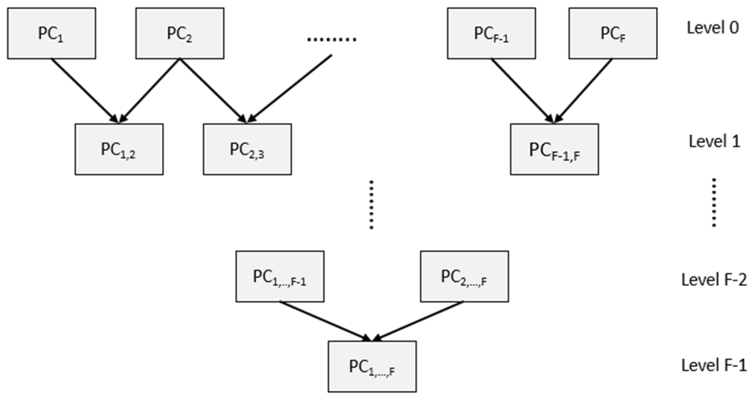
In this experiment, the size of the original image in each view was randomly sampled to 60% with the assumption that there was an overlap between each consecutive view. The voxel hull method [63,64,65] was used to select representative points inside the overlapping area. After that, the registration process with the parameter setting shown in Table 2 was implemented. Since there were six consecutive views, the hierarchical registration with F = 6 was used to increase the registration performance shown in Figure 4. The survival at each level was the best final registration result (BCDL-GWO algorithm with the ICP method), and that result proceeded to the next level of the hierarchical registration.
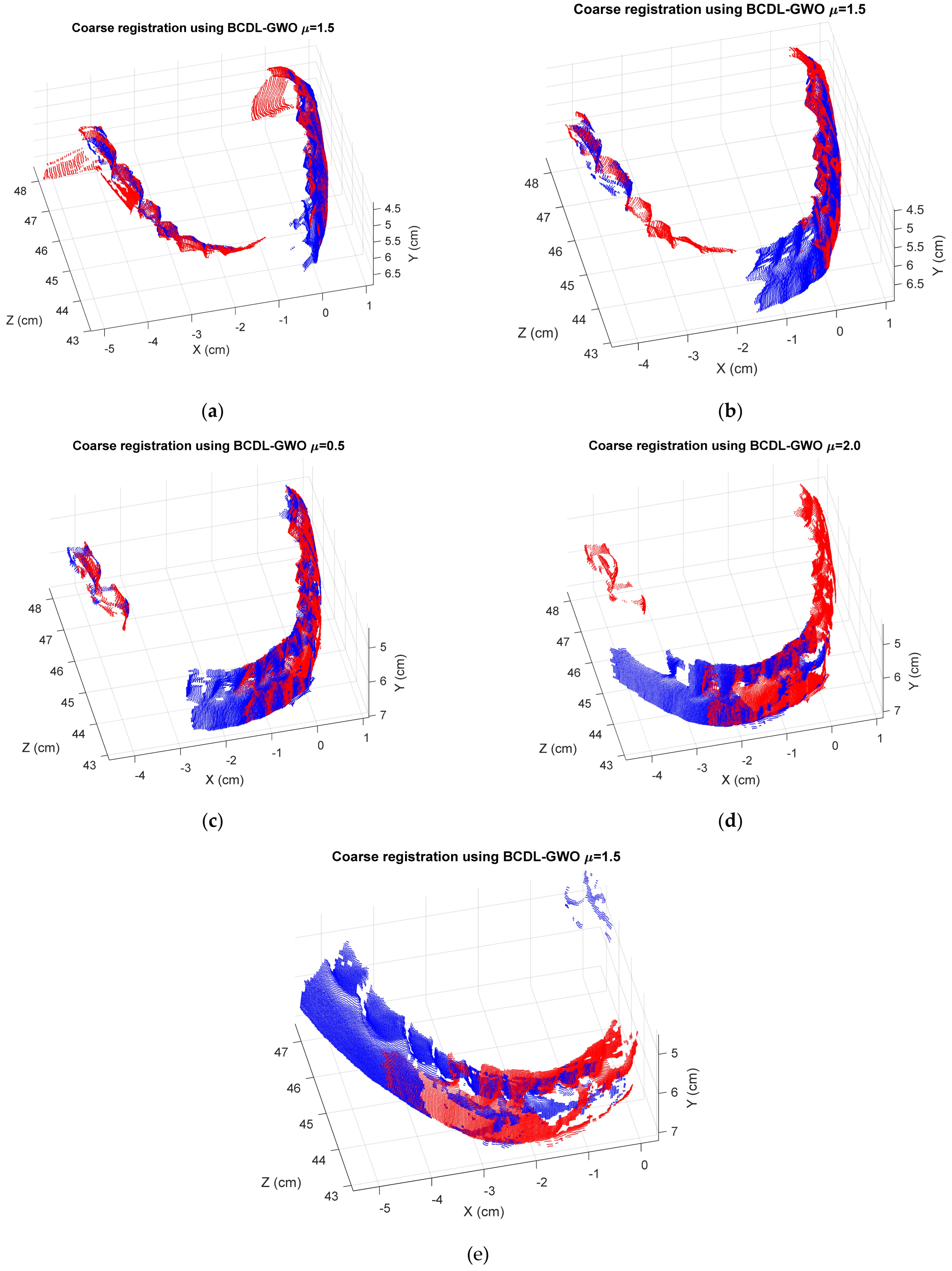
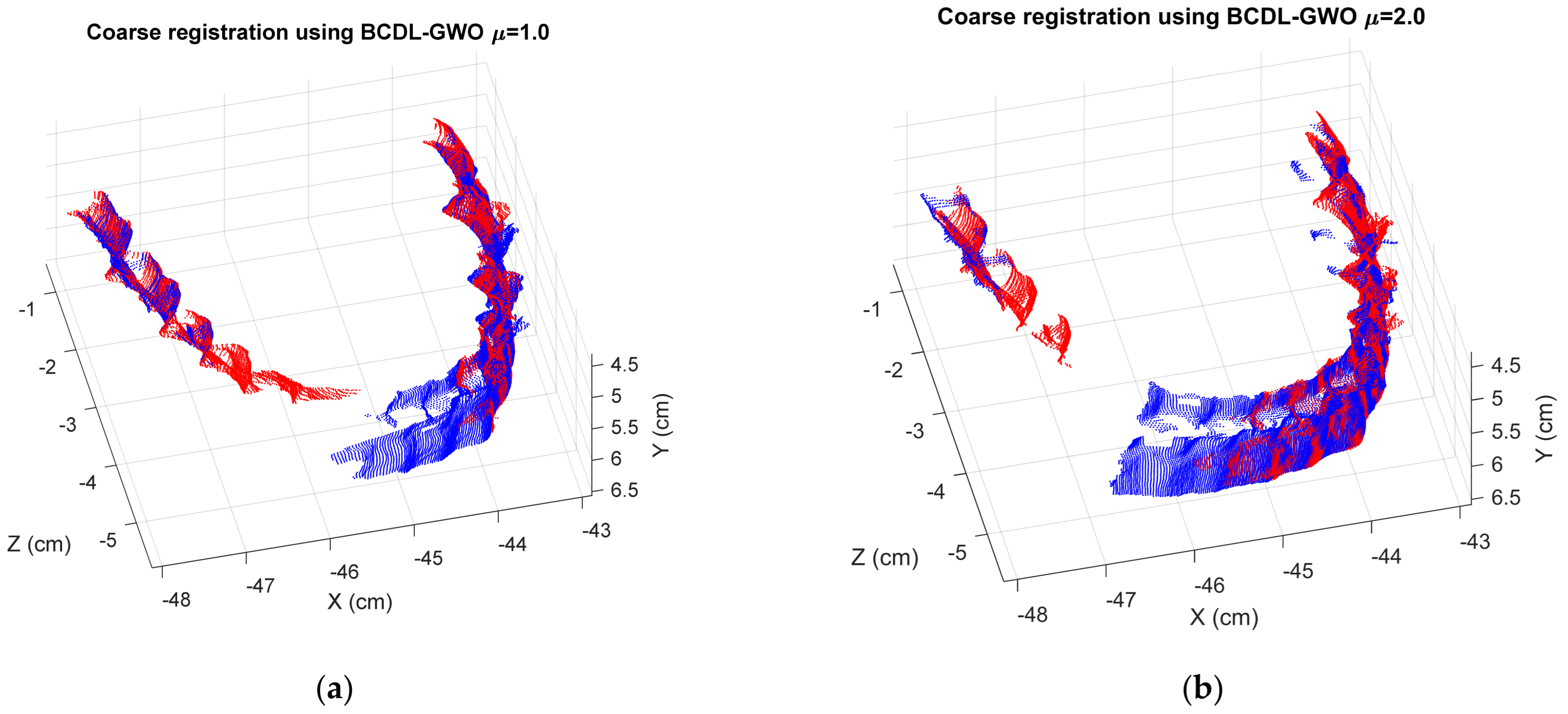
Table 11 shows the registration MSE results from the BCDL-GWO without the ICP of the regular tooth model at hierarchical level 1, whereas those with ICP are shown in Table 12. Figure 5 and Figure 6 show the best registration of each consecutive pair without and with ICP, respectively.
We compare our results with those from SR-PSO [39] as well. The MSEs of the regular tooth model at hierarchical level 1 are shown in Table 13. From the results, we can see that both methods provide comparable results. However, when we look at the MSEs of the final 3D reconstruction of the regular tooth model from six consecutive views shown in Table 14, we can see that the results from the best BCDL-GWO with ICP (7.2186 μm2 when μ = 0.5) are better than SR-PSO with ICP (7.3666 μm2).
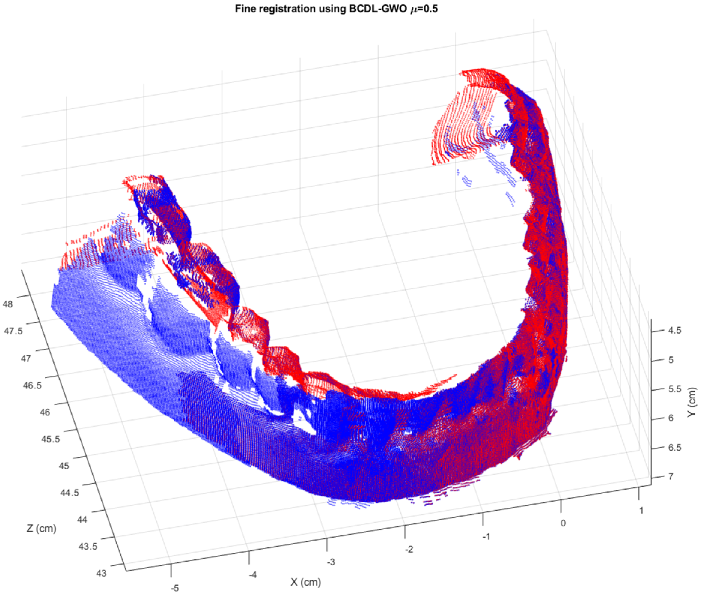
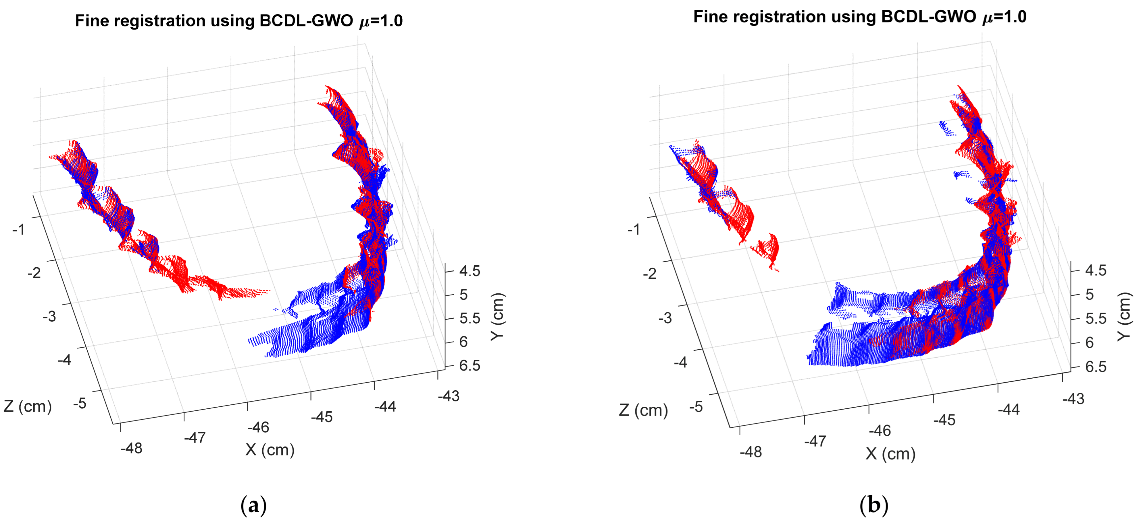
The final registration of the regular tooth model is shown in Figure 7. We can see that the reconstruction result provides a good visualization.
Finally, we implement the BCDL-GWO on the orthodontic tooth model to observe more experiments. The MSE registration results at hierarchical level 1 from the BCDL-GWO and BCDL-GWO with the ICP are shown in Table 15 and Table 16, respectively. Figure 8 and Figure 9 show the best registration results for each consecutive pair.
Again, we compare our MSEs on the registration results with those from the SR-PSO, as shown in Table 17. We can see that our proposed algorithm without the ICP method provides better registration results than the SR-PSO without the ICP method, except for a pair of 2 vs. 3. However, for the fine registration, our BCDL-GWO with ICP is comparable with those from the SR-PSO with ICP. But when we look at the final registration 3D orthodontic reconstruction model, as shown in Table 18, the results from the BCDL-GWO with ICP are better than the best results from the SR-PSO with ICP (7.4130 μm2). While the best result from the BCDL-GWO with ICP at μ = 1.5 is 7.3999 μm2. The final 3D reconstruction of the orthodontic tooth model is shown in Figure 10. We can see that the reconstruction result can still provide a good visualization.
To confirm that our method is good enough, we indirectly compare our results with those existing methods in the literature on the dental 3D registration data sets. However, those methods were performed on different data sets. The comparison results are shown in Table 19. Again, the results from our BCDL-GWO are better.
One might wonder what the computational complexity of BCDL-GWO is compared with the SR-PSO, BOA, HHO, SMA, and WOA shown in Table 20. To compute the complexity of the BCDL-GWO, we start with the population initialization step. Since there are K grey wolves in the population and each grey wolf is represented by a D-dimensional vector, the computational complexity in this step is O(K × D). For the control parameter step, the first operation is the GWO-SCA, which needs O(K × D). The next operation in this step is Equation (15), which will need O(D). Then, both the position update and fitness evaluation will need O(K × D). Hence, in this step, it is O(K × D). However, in the fitness comparison step, it will need O(K). The next step is the behavior consideration procedure. In this step, the new candidate solution calculation from Equation (26) will need O(K × D). The fitness calculation in this step will need O(K × D). The update position using Equation (27) will be O(K × D). Hence, in this step, the complexity will be O(K × D). Finally, in the dimensional learning procedure step, the distance calculation will need O(K × D). Equation (29) used in the search agents will need O(K × D2). Again, the position update needs O(K × D). However, in this step, the total complexity is O(K × D2). Since there are T iterations, the total complexity of the BCDL-GWO will be O(T × K × D2). For other algorithms, the complexities are calculated similarly. Table 20 shows the Big O of each step in each algorithm. The complexities of all algorithms are very similar. Even though the BCDL-GWO has a slightly higher complexity than the others, the tradeoff with the performance of our BCDL-GWO is still good.

4. Conclusions

To help in dental diagnostic and treatment planning in rural areas with limited access to sophisticated devices, a 3D reconstruction from multi-view optical images is needed. To provide a good 3D reconstruction, a good 3D registration process is required. In this paper, we developed the grey wolf optimization algorithm with behavior considerations and dimensional learning strategies (BCDL-GWO) with iterative closet point (ICP) to find the optimal affine transform in the 3D registration process. We compare the results with those from the statistical randomization-based particle swarm optimization (SR-PSO). We found that the final best result of BCDL-GWO with the ICP yields a mean squared error (MSE) of 7.2186 μm2 for 3D reconstruction from six consecutive views of the regular tooth model, whereas that of SR-PSO with the ICP method is 7.3666 μm2. The MSE of the BCDL-GWO with the ICP method is 7.3999 μm2 for the orthodontic tooth model, while the SR-PSO with the ICP provides 7.4130 μm2. We can say that the 3D reconstruction of the regular and orthodontic tooth models from the BCDL-GWO with ICP is better than the SR-PSO with ICP.
We also estimate the computational complexity of both the BCDL-GWO and the SR-PSO. We could say that they are comparable. However, from the nature of the BCDL-GWO, we can also say that it can cope with a premature convergence, an unbalance between exploration and exploitation, and finally, it increases a pack’s diversity.
Currently, there is only one research work involving the 3D model to assess dental caries [70]. This shows that there is a need for a 3D model for dental caries assessment. Hence, in future work, we plan to implement our algorithm in order to simulate dental caries for tooth defections in real situations.

Author Contributions

All authors conceived and designed the experiments; R.W. performed the experiments; and all authors contributed to the writing of the paper. All authors have read and agreed to the published version of the manuscript.

Funding

This research was funded by the Royal Golden Jubilee Ph.D. Program (Grant No. PHD-0170-2558).

Institutional Review Board Statement

Not applicable.

Informed Consent Statement

Not applicable.

Data Availability Statement

No new data were created or analyzed in this study. Data sharing is not applicable to this article.

Acknowledgments

The authors would like to thank the Royal Golden Jubilee Ph.D. Program (RGJ-PhD) for support under grant No. PHD-0170-2558 for financial funding.

Conflicts of Interest

The authors of the paper do not have any conflicts of interest with any companies or institutions. This work was supported by the Thailand Research Fund under the Royal Golden Jubilee Ph.D. Program (Grant No. PHD-0170-2558). This article does not contain any studies with human participants or animals performed by any of the authors.

References

  1. Sivakumar, A.; Thangaswamy, V.; Ravi, V. Treatment planning in conservative dentistry. J. Pharm. Bioallied Sci. 2012, 4 (Suppl. S2), S406–S409. [Google Scholar] [CrossRef] [PubMed]
  2. Stefanac, S.; Nesbit, S. Diagnosis and Treatment Planning in Dentistry, 3rd ed.; Elsevier: Amsterdam, The Netherlands, 2017; ISBN 9780323287302. [Google Scholar]
  3. Hugar, S.M.; Sogi, H.P.S.; Nalawade, T.M.; Sinha, A.; Hugar, S.; Mallikarjuna, R.M. Knowledge, attitude, and practices of oral health care in prevention of early childhood caries among parents of children in Belagavi city: A Questionnaire study. J. Fam. Med. Prim. Care 2016, 5, 286–290. [Google Scholar] [CrossRef] [PubMed]
  4. Yanagisawa, R.; Sugaya, Y.; Kasahara, S.; Omachi, S. Tooth shape reconstruction from dental CT images with the region-growing method. Dentomaxillofacial Radiol. 2014, 43, 20140080. [Google Scholar] [CrossRef]
  5. Zhou, X.; Gan, Y.; Xiong, J.; Zhang, D.; Zhao, Q.; Xia, Z. A Method for Tooth Model Reconstruction Based on Integration of Multimodal Images. J. Healthc. Eng. 2018, 2018, 4950131. [Google Scholar] [CrossRef]
  6. Zhang, D.; Gan, Y.; Xiong, J.; Xia, Z. Three-dimensional tooth model reconstruction based on fusion of dental computed tomography images and laser-scanned images (Chineses Article). Shengwu Yixue Gongchengxue Zazhi 2017, 34, 7–14. (In Chinese) [Google Scholar]
  7. Yau, H.-T.; Yang, T.-J.; Chen, Y.-C. Tooth model reconstruction based upon data fusion for orthodontic treatment simulation. Comput. Biol. Med. 2014, 48, 8–16. [Google Scholar] [CrossRef] [PubMed]
  8. Martorelli, M.; Ausiello, P. A novel approach for a complete 3D tooth reconstruction using only 3D crown data. Int. J. Interact. Des. Manuf. 2013, 7, 125–133. [Google Scholar] [CrossRef]
  9. Gan, Y.; Tan, J.; Zhao, Q.; Xia, Z. Automatic 3D Tooth Model Reconstruction from CT Images. In Proceedings of the 2014 International Association for Dental Research/Asia Pacific Region (IADR/APR), Cape Town, South Africa, 25 June 2014. [Google Scholar]
  10. Srisilapanan, P.; Nirunsittirat, A.; Roseman, J. Trends over Time in Dental Caries status in Urban and Rural Thai Children. J. Clin. Exp. Dent. 2017, 9, e1201–e1206. [Google Scholar] [CrossRef]
  11. Abdel-Basset, M.; Fakhry, A.E.; El-henawy, I.; Qiu, T.; Sangaiah, A.K. Feature and Intensity Based Medical Image Registration Using Particle Swarm Optimization. J. Med. Syst. 2017, 41, 197. [Google Scholar] [CrossRef]
  12. Sarvamangala, D.R.; Kulkarni, R.V. Swarm Intelligence Algorithms for Medical Image Registration: A Comparative Study. Commun. Comput. Inf. Sci. 2017, 776, 451–465. [Google Scholar] [CrossRef]
  13. Khan, M.K.; Nystrom, I. A Modified Particle Swarm Optimization Applied in Image Registration. In Proceedings of the 2010 20th International Conference on Pattern Recognition, Istanbul, Turkey, 23–26 August 2010; IEEE: Piscataway Township, NJ, USA, 2010; pp. 2302–2305. [Google Scholar]
  14. Jara, R.I.; Buchelly, F.J.; Meschino, G.; Ballarin, V.L. Improved Particle Swarm Optimization algorithm applied to rigid registration in medical images. In Proceedings of the VII Latin American Congress on Biomedical Engineering CLAIB 2016, Bucaramanga, Santander, Colombia, 26–28 October 2016; IFMBE Proceedings. Torres, I., Bustamante, J., Sierra, D., Eds.; Springer: Singapore, 2016; Volume 60, pp. 161–164. [Google Scholar]
  15. Yonghong, Y.; Jiying, L.; Qiang, W.; Tao, Z. Improved Particle Swarm Optimization Image Registration Based on Mutual Information. In Proceedings of the 2019 11th International Conference on Measuring Technology and Mechatronics Automation (ICMTMA), Qiqihar, China, 28–29 April 2019; IEEE: Piscataway Township, NJ, USA, 2019; pp. 450–453. [Google Scholar]
  16. Ramirez, L.; Durdle, N.G.; Raso, V.J. A Parameters Selection Scheme for Medical Image Registration. In Proceedings of the Annual Meeting of the North American Fuzzy Information Processing Society (NAFIPS), Montreal, QC, Canada, 3–6 June 2006; pp. 505–510. [Google Scholar]
  17. Sabuncu, M.R.; Ramadge, P.J. Spatial Information in Entropy-Based Image Registration. In WBIR 2003, Lecture Notes in Computer Science; Gee, J.C., Maintz, J.B.A., Vannier, M.W., Eds.; Springer: Berlin/Heidelberg, Germany, 2003; Volume 2717. [Google Scholar] [CrossRef]
  18. Kaur, A.; Kaur, L.; Gupta, S. Image Recognition using Coefficient of Correlation and Structural Similarity Index in Uncontrolled Environment. Int. J. Comput. Appl. 2012, 59, 32–39. [Google Scholar] [CrossRef]
  19. Daniel, E.; Anitha, J.; Kamaleshwaran, K.K.; Rani, I. Optimum spectrum mask based medical image fusion using Grey Wolf Optimization. Biomed. Signal Process. Control 2017, 34, 36–43. [Google Scholar] [CrossRef]
  20. Dida, H.; Charif, F.; Benchabane, A. Grey Wolf Optimizer for Multimodal Medical Image Registration. In Proceedings of the Fourth International Conference on Intelligent Computing in Data Sciences (ICDS), Fez, Morocco, 21–23 October 2020; pp. 1–5. [Google Scholar] [CrossRef]
  21. Chakraborty, S.; Pradhan, R.; Ashour, A.S.; Moraru, L.; Dey, N. Grey-Wolf-Based Wang’s Demons for Retinal Image Registration. Entropy 2020, 22, 659. [Google Scholar] [CrossRef]
  22. Shaw, K.; Pandey, P.; Das, S.; Ghosh, D.; Malakar, P.; Dhabal, S. Image Registration using Bio-inspired Algorithms. In Proceedings of the 2020 IEEE 1st International Conference for Convergence in Engineering (ICCE), Kolkata, India, 5–6 September 2020; pp. 330–334. [Google Scholar] [CrossRef]
  23. Yan, X.; Zhang, Y.; Zhang, D.; Hou, N. Multimodal image registration using histogram of oriented gradient distance and data-driven grey wolf optimizer. Neurocomputing 2020, 392, 108–120. [Google Scholar] [CrossRef]
  24. Lazar, Đ.; Jokic, A.; Petrovic, M.; Miljković, Z. Biologically Inspired Optimization Methods for Image Registration in Visual Servoing of a Mobile Robot. In Proceedings of the 7th International Conference on Electrical, Electronic and Computing Engineering (IcETRAN), Etno-Selo Stanišići, Republika Srpska, 28–30 September 2020. [Google Scholar]
  25. Kaur, K.; Budhiraja, S.; Sharma, N. Multimodal Medical Image Fusion based on Gray Wolf Optimization and Hilbert Transform. Biomed. Pharmacol. J. 2019, 12, 2091–2098. [Google Scholar] [CrossRef]
  26. Dida, H.; Charif, F.; Benchabane, A. Registration of computed tomography images of a lung infected with COVID-19 based in the new meta-heuristic algorithm HPSGWO. Multimed. Tools Appl. 2022, 81, 18955–18976. [Google Scholar] [CrossRef]
  27. Wachowiak, M.P.; Smolíková, R.; Zheng, Y.; Zurada, J.M.; Elmaghraby, A.S. An Approach to Multimodal Biomedical Im-age Registration Utilizing Particle Swarm Optimization. IEEE Trans. Evol. Comput. 2004, 8, 289–301. [Google Scholar] [CrossRef]
  28. Chen, Y.-W.; Mimori, A. Hybrid Particle Swarm Optimization for Medical Image Registration. In Proceedings of the 2009 Fifth International Conference on Natural Computation, Tianjian, China, 14–16 August 2009; IEEE: Piscataway Township, NJ, USA, 2009; Volume 6, pp. 26–30. [Google Scholar]
  29. Abduo, J.; Bennamoun, M. Three-dimensional image registration as a tool for forensic odontology: A preliminary investigation. Am. J. Forensic Med. Pathol. 2013, 34, 260–266. [Google Scholar] [CrossRef] [PubMed]
  30. Wu, C.; Bradley, D.; Garrido, P.; Zollhöfer, M.; Theobalt, C.; Gross, M.; Beeler, T. Model-based teeth reconstruction. ACM Trans. Graph. 2016, 35, 220. [Google Scholar] [CrossRef]
  31. Yamany, S.M.; Farag, A.A.; Tasman, D.; Farman, A.G. A 3-D reconstruction system for the human jaw using a sequence of optical images. IEEE Trans. Med. Imaging 2000, 19, 538–547. [Google Scholar] [CrossRef] [PubMed]
  32. Zhan, X.; Cai, Y.; He, P. A three-dimensional point cloud registration based on entropy and particle swarm optimization. Adv. Mech. Eng. 2018, 10, 1687814018814330. [Google Scholar] [CrossRef]
  33. Zhan, X.; Cai, Y.; Li, H.; Li, Y.; He, P. A point-cloud registration algorithm based on normal vector and particle swarm optimization. Meas. Control 2019, 53, 265–275. [Google Scholar] [CrossRef]
  34. Ge, Y.; Wang, B.; Nie, J.; Sun, B. A point cloud registration method combining enhanced particle swarm optimization and iterative closest point method. In Proceedings of the 2016 Chinese Control and Decision Conference (CCDC), Yinchuan, China, 28–30 May 2016; IEEE: Piscataway Township, NJ, USA, 2016; pp. 2810–2815. [Google Scholar]
  35. Yousry, M.; Youssef, B.A.B.; El Aziz, M.A.; Sidky, F.I. 3D Point-cloud Registration Using Particle Swarm Optimization Based on Different Descriptors. Int. J. Sci. Eng. Res. 2017, 8, 558–564. [Google Scholar]
  36. John, V.; Xu, Y.; Mita, S.; Long, Q.; Liu, Z.; Tan, Y.; Takagi, H.; Shi, Y. Registration of GPS and Stereo Vision for Point Cloud Localization in Intelligent Vehicles Using Particle Swarm Optimization. In Lecture Notes in Computer Science; Springer International Publishing: Berlin/Heidelberg, Germany, 2017; Volume 10385, pp. 209–217. [Google Scholar]
  37. Zhang, L.; Yang, B.; Wang, L.; Zhao, X.; Zhou, J.; Li, M.; Han, Y. Three-dimensional Cement Image Registration Based on Multi-layer PSO and Mutual Information. In Proceedings of the 2016 3rd International Conference on Informative and Cybernetics for Computational Social Systems (ICCSS), Jinzhou, China, 26–29 August 2016. [Google Scholar]
  38. Feng, Y.; Tang, J.; Su, B.; Su, Q.; Zhou, Z. Point Cloud Registration Algorithm Based on the Grey Wolf Optimizer. IEEE Access 2020, 8, 143375–143382. [Google Scholar] [CrossRef]
  39. Wongkhuenkaew, R.; Auephanwiriyakul, S.; Chaiworawitkul, M.; Theera-Umpon, N. Three-Dimensional Tooth Model Reconstruction Using Statistical Randomization-Based Particle Swarm Optimization. Appl. Sci. 2021, 11, 2363. [Google Scholar] [CrossRef]
  40. Mirjalili, S.; Mirjalili, S.M.; Lewis, A. Grey wolf optimizer. Adv. Eng. Softw. 2014, 69, 46–61. [Google Scholar] [CrossRef]
  41. Singh, N.; Singh, S.B. A novel hybrid GWO-SCA approach for optimization problems. Eng. Sci. Technol. Int. J. 2017, 20, 1586–1601. [Google Scholar] [CrossRef]
  42. Heidari, A.A.; Pahlavani, P. An efficient modified grey wolf optimizer with Lévy flight for optimization tasks. Appl. Soft Comput. 2017, 60, 115–134. [Google Scholar] [CrossRef]
  43. Long, W.; Jiao, J.; Liang, X.; Cai, S.; Xu, M. A Random Opposition-Based Learning Grey Wolf Optimizer. IEEE Access 2019, 7, 113810–113825. [Google Scholar] [CrossRef]
  44. Nadimi-Shahraki, M.H.; Taghian, S.; Mirjalili, S. An improved grey wolf optimizer for solving engineering problems. Expert Syst. Appl. 2021, 166, 113917. [Google Scholar] [CrossRef]
  45. Wang, F.; Zhao, Z. A survey of iterative closest point algorithm. In Proceedings of the Chinese Automation Congress (CAC), Jinan, China, 20–22 October 2017; IEEE: Piscataway Township, NJ, USA, 2017; pp. 4395–4399. [Google Scholar] [CrossRef]
  46. Duda, R.O.; Hart, P.E.; Stork, D.G. Pattern Classification, 2nd ed.; John Willey & Sons: Hoboken, NJ, USA, 2001. [Google Scholar]
  47. Chen, Y.; Medioni, G. Object modelling by registration of multiple range images. Image Vis. Comput. 1992, 10, 145–155. [Google Scholar] [CrossRef]
  48. FitzGibbon, A.W. Robust registration of 2D and 3D point sets. Image Vis. Comput. 2003, 21, 1145–1153. [Google Scholar] [CrossRef]
  49. Rezaei, F.; Safavi, H.R.; Abd Elaziz, M.; El-Sappagh, S.H.A.; Al-Betar, M.A.; Abuhmed, T. An Enhanced Grey Wolf Optimizer with a Velocity-Aided Global Search Mechanism. Mathematics 2022, 10, 351. [Google Scholar] [CrossRef]
  50. Long, W.; Jiao, J.; Liang, X.; Tang, M. An exploration-enhanced grey wolf optimizer to solve high-dimensional numerical optimization. Eng. Appl. Artif. Intell. 2018, 68, 63–80. [Google Scholar] [CrossRef]
  51. Gao, Z.-M.; Zhao, J. An Improved Grey Wolf Optimization Algorithm with Variable Weights. Comput. Intell. Neurosci. 2019, 2019, 2981282. [Google Scholar] [CrossRef]
  52. Qiao, Y.; Hsu, H.-Y.; Pan, J.-S. Behavior-based Grey Wolf Optimizer for Wireless Sensor Network Deployment Problem. Int. J. Ad Hoc Ubiquitous Comput. 2022, 39, 70–82. [Google Scholar] [CrossRef]
  53. Yang, X.-S. Nature-Inspired Metaheuristic Algorithms, 2nd ed.; Luniver Press: England, UK, 2010; ISBN 1-905986-28-9. [Google Scholar]
  54. Kennedy, J.; Eberhart, R. Particle swarm optimization. In Proceedings of the International Conference on Neural Networks (ICNN), Perth, WA, Australia, 27 November–1 December 1995; pp. 1942–1948. [Google Scholar] [CrossRef]
  55. Besl, P.; McKay, N.D. A method for registration of 3-D shapes. IEEE Trans. Pattern Anal. Mach. Intell. 1992, 14, 239–256. [Google Scholar] [CrossRef]
  56. Lagarias, J.C.; Reeds, J.A.; Wright, M.H.; Wright, P.E. Convergence Properties of the Nelder-Mead Simplex Method in Low Dimensions. SIAM J. Optim. 1998, 9, 112–147. [Google Scholar] [CrossRef]
  57. Arora, S.; Singh, S. Butterfly optimization algorithm: A novel approach for global optimization. Soft Comput. 2019, 23, 715–734. [Google Scholar] [CrossRef]
  58. Heidari, A.A.; Mirjalili, S.; Faris, H.; Aljarah, I.; Mafarja, M.; Chen, H. Harris hawks optimization: Algorithm and applications. Future Gener. Comput. Syst. 2019, 97, 849–872. [Google Scholar] [CrossRef]
  59. Li, S.; Chen, H.; Wang, M.; Asghar Heidari, A.A.; Mirjalili, S. Slime mould algorithm: A new method for stochastic optimization. Future Gener. Comput. Syst. 2020, 111, 300–323. [Google Scholar] [CrossRef]
  60. Mirjalili, S.; Lewis, A. The Whale Optimization Algorithm. Adv. Eng. Softw. 2016, 111, 300–323. [Google Scholar] [CrossRef]
  61. Li, P.; Wang, R.; Wang, Y.; Gao, G. Fast Method of Registration for 3D RGB Point cloud with Improved Four Initial Point Pairs Algorithm. Sensors 2020, 20, 138. [Google Scholar] [CrossRef]
  62. Du, S.; Zheng, N.; Xiong, L.; Ying, S.; Xue, J. Scaling iterative closest point algorithm for registration of m–D point sets. J. Vis. Commun. Image Represent. 2010, 21, 442–452. [Google Scholar] [CrossRef]
  63. Glira, P.; Pfeifer, N.; Ressl, C.; Briese, C. A correspondence framework for ALS strip adjustments based on variants of the ICP algorithm. J. Photogramm. Remote Sens. Geoinf. Sci. (PFG) 2015, 4, 275–289. [Google Scholar] [CrossRef]
  64. Glira, P.; Pfeifer, N.; Ressl, C.; Briese, C. Rigorous Strip Adjustment of Airborne Laser scanning Data Based on the ICP Algorithm. ISPRS Ann. Photogramm. Remote Sens. Spat. Inf. Sci. 2015, 2, 73–80. [Google Scholar] [CrossRef]
  65. Point Cloud Tools for Matlab. Available online: www.geo.tuwien.ac.at/downloads/pg/pctools/pctools.html (accessed on 12 May 2022).
  66. Kalla, M.-P.; Economopoulos, T.L.; Matsopoulos, G.K. 3D dental image registration using exhaustive deformable models: A comparative study. Dentomaxillofacial Radiol. 2017, 46, 20160390. [Google Scholar] [CrossRef]
  67. Kim, M.; Chung, M.; Shin, Y.-G.; Kim, B. Automatic registration of dental CT and 3D scanned model using deep split jaw and surface curvature. Comput. Methods Programs Biomed. 2023, 233, 107467. [Google Scholar] [CrossRef]
  68. Kurniawan, A.; Yodokawa, K.; Kosaka, M.; Ito, K.; Sasaki, K.; Aoki, T.; Suzuki, T. Determining the effective number and surfaces of teeth for forensic dental identification through the 3D point cloud data analysis. Egypt. J. Forensic Sci. 2020, 10, 3. [Google Scholar] [CrossRef]
  69. Chung, M.; Lee, J.; Song, W.; Song, Y.; Yang, I.-H.; Lee, J.; Shin, Y.-G. Automatic Registration Between Dental Cone-Beam CT and Scanned Surface via Deep Pose Regression Neural Networks and Clustered Similarities. IEEE Trans. Med. Imaging 2020, 32, 3900–3909. [Google Scholar] [CrossRef]
  70. Porumb, I.C.; Leucuta, D.C.; Nigoghossian, M.; Culic, B.; Lucaciu, P.O.; Culic, C.; Badea, I.C.; Leghezeu, A.N.; Nicoara, A.G.; Simu, M.R. Caries Lesion Assessment Using 3D Virtual Models by Examiners with Different Degrees of Clinical Experience. Medicina 2023, 59, 2157. [Google Scholar] [CrossRef]
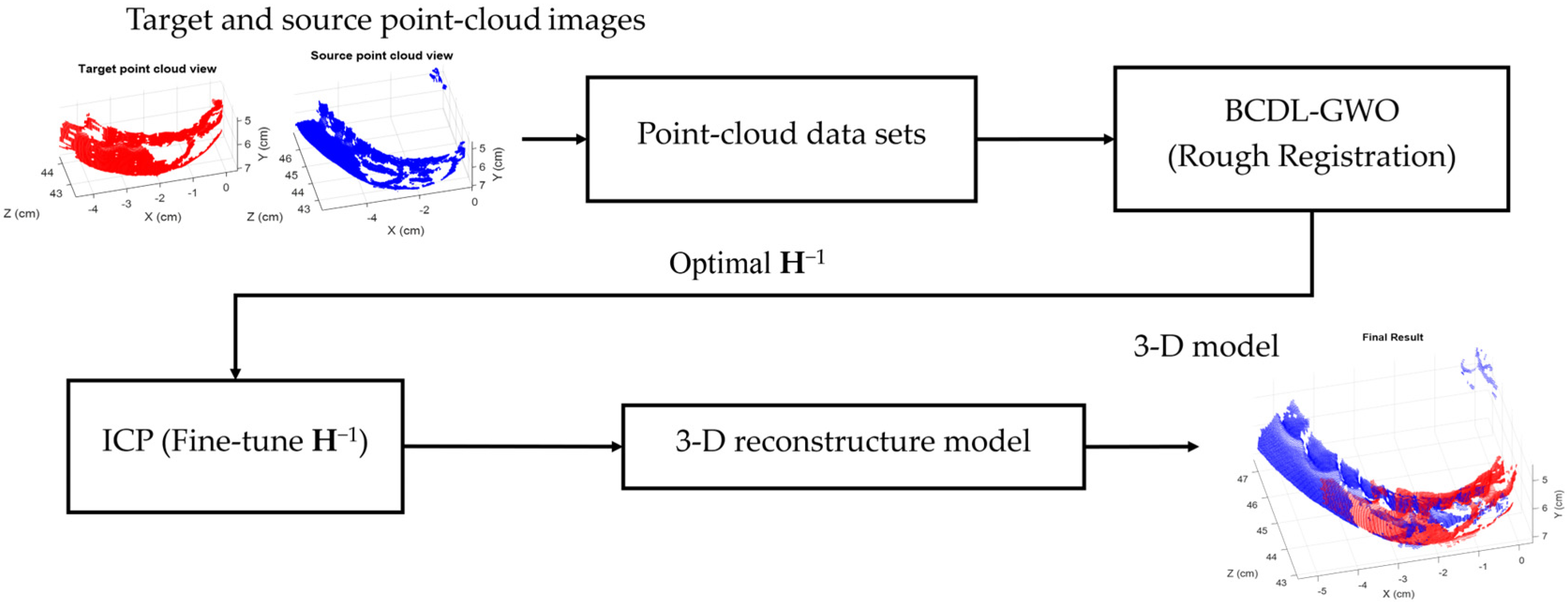
Figure 1. Three-dimensional reconstruction with BCDL-GWO.
Bioengineering 11 00254 g001
Figure 2. The original shape (target point cloud) and the 3D transformation (source point cloud) of (a) synthetic cylindrical and (b) synthetic pyramid shapes.
Bioengineering 11 00254 g002
Figure 3. The final best registration using BCDL-GWO with μ = 0.5 of synthetic (a) cylindrical and (b) pyramid images.
Bioengineering 11 00254 g003
Figure 4. Hierarchical structure for multiple-views registration.
Bioengineering 11 00254 g004
Figure 5. The best registration results of BCDL-GWO only for the following pairs: (a) 1 and 2; (b) 2 and 3; (c) 3 and 4; (d) 4 and 5; (e) 5 and 6.
Bioengineering 11 00254 g005
Figure 6. The best registration results of BCDL-GWO with ICP for the following pairs: (a) 1 and 2; (b) 2 and 3; (c) 3 and 4; (d) 4 and 5; (e) 5 and 6.
Bioengineering 11 00254 g006
Figure 7. The final registration result of six consecutive views of the regular tooth model from the BCDL-GWO with the ICP.
Bioengineering 11 00254 g007
Figure 8. The best registration results of BCDL-GWO for the following pairs: (a) 1 and 2; (b) 2 and 3; (c) 3 and 4; (d) 4 and 5; (e) 5 and 6.
Bioengineering 11 00254 g008aBioengineering 11 00254 g008b
Figure 9. The best registration results of BCDL-GWO with ICP for the following pairs: (a) 1 and 2; (b) 2 and 3; (c) 3 and 4; (d) 4 and 5; (e) 5 and 6.
Bioengineering 11 00254 g009aBioengineering 11 00254 g009b
Figure 10. The final registration result of six consecutive views of the orthodontic tooth model from the BCDL-GWO with the ICP.
Bioengineering 11 00254 g010
Table 1. Parameters boundaries in optimization process.
ParametersLower BoundUpper Bound
tx, ty, tz−1.5 (cm)1.5 (cm)
ϕx, ϕy, ϕz−45 (deg)45 (deg)
sx, sy, sz0.8 (20% downscaling)1.2 (20% upscaling)
sh1, sh2, sh3, sh4, sh5, sh6−0.5 (cm)0.5 (cm)
Table 2. BCDL-GWO parameters configuration.
ParametersSymbolsValues
Search agents (wolves)K100
IterationsT2000
Control parameter aa02
Control parameter cc02
Nonlinear exponent indicesμ0.5, 1.0, 1.5, 2.0
Lévy distributionβ1.5
Table 3. The mean squared error (MSE) in pixels2 of the registration on the synthetic cylindrical shape.
Research work in [39]α
α = 0.5α = 1.0α = 1.5α = 2.0
Without ICP7.68 × 10−29.23 × 10−23.22 × 10−319.68 × 10⁻²
With ICP7.68 × 10−29.23 × 10−23.22 × 10−319.68 × 10⁻²
BCDL-GWOμ
0.51.01.52.0
Without ICP1.90 × 10−95.37 × 10−113.46 × 10−133.23 × 10⁻¹²
With ICP2.71 × 10−277.35 × 10−224.11 × 10−263.41 × 10⁻²¹
Table 4. The mean squared error (MSE) in pixels2 of the registration on the synthetic pyramid shape.
SR-PSO [39]α
α = 0.5α = 1.0α = 1.5α = 2.0
Without ICP1.14 × 10−31.18 × 10−45.71 × 10−301.70 × 10⁻⁴
With ICP1.51 × 10−179.66 × 10−185.71 × 10−306.97 × 10⁻¹⁸
BCDL-GWOμ
0.51.01.52.0
Without ICP9.37 × 10−103.40 × 10−101.96 × 10−131.95 × 10⁻¹²
With ICP7.79 × 10−201.23 × 10−181.63 × 10−176.51 × 10⁻¹⁸
Table 5. The average registration mean squared error (MSE) ± standard deviation in pixels2 on the synthetic cylindrical shape.
SR-PSO [39]α
α = 0.5α = 1.0α = 1.5α = 2.0
Without ICP5.38 × 10−2
± 3.73 × 10⁻²
4.66 × 10⁻²
± 4.05 × 10⁻²
3.84 × 10⁻²
± 4.06 × 10⁻²
5.56 × 10⁻²
± 3.90 × 10⁻²
With ICP5.38 × 10−2
± 3.73 × 10⁻²
4.66 × 10⁻²
± 4.05 × 10⁻²
3.84 × 10⁻²
± 4.06 × 10⁻²
5.56 × 10⁻²
± 3.90 × 10⁻²
BCDL-GWOμ
0.51.01.52.0
Without ICP2.91 × 10−9
± 3.73 × 10⁻⁹
1.14 × 10⁻¹⁰
± 1.7 × 10⁻¹⁰
1.07 × 10⁻¹¹
± 1.67 × 10⁻¹¹
1.19 × 10⁻¹¹
± 2.26 × 10⁻¹¹
With ICP1.68 × 10−19
± 4.48 × 10⁻¹⁹
4.26 × 10⁻²²
± 1.03 × 10⁻²¹
2.64 × 10⁻¹⁹
± 8.31 × 10⁻¹⁹
5.69 × 10⁻²⁰
± 1.17 × 10⁻¹⁹
Table 6. The average registration mean squared error (MSE) ± standard deviation in pixels2 on the synthetic pyramid shape.
SR-PSO [39]α
α = 0.5α = 1.0α = 1.5α = 2.0
Without ICP1.65 × 10−4
± 3.68 × 10⁻⁴
4.92 × 10⁻⁵
± 1.08 × 10⁻⁴
1.92 × 10⁻⁶
± 6.08 × 10⁻⁶
1.71 × 10⁻⁵
± 5.38 × 10⁻⁵
With ICP2.83 × 10−18
± 5.91 × 10⁻¹⁸
4.90 × 10⁻¹⁹
± 1.55 × 10⁻¹⁸
5.71 × 10⁻¹⁸
± 1.81 × 10⁻¹⁷
9.92 × 10⁻¹⁸
± 2.79 × 10⁻¹⁷
BCDL-GWOμ
0.51.01.52.0
Without ICP2.30 × 10−9
± 4.76 × 10⁻⁹
6.29 × 10⁻¹⁰
± 9.14 × 10⁻¹⁰
2.49 × 10⁻¹⁰
± 7.04 × 10⁻¹⁰
7.35 × 10⁻¹²
± 1.76 × 10⁻¹¹
With ICP2.15 × 10−16
± 6.56 × 10⁻¹⁶
3.79 × 10⁻¹⁸
± 4.78 × 10⁻¹⁸
5.79 × 10⁻¹⁸
± 9.57 × 10⁻¹⁸
6.93 × 10⁻¹⁹
± 2.05 × 10⁻¹⁸
Table 7. The best average registration mean squared error (MSE) ± standard deviation in pixels2 on the synthetic cylindrical shapes.
BOA [57]HNO [58]SMA [59]WOA [60]SR-PSO [39]BCDL-GWO
Without ICP1.08 × 10−1
± 3.83 × 10⁻³
9.63 × 10⁻²
± 7.49 × 10⁻³
4.78 × 10⁻²
± 4.70 × 10⁻²
7.27 × 10⁻²
± 1.99 × 10⁻²
3.84 × 10⁻²
± 4.06 × 10⁻²
1.07 × 10⁻¹¹
± 1.67 × 10⁻¹¹
With ICP8.58 × 10−2
± 1.35 × 10⁻²
8.84 × 10⁻²
± 1.09 × 10⁻²
4.54 × 10⁻²
± 4.79 × 10⁻²
6.16 × 10⁻²
± 3.38 × 10⁻²
3.84 × 10⁻²
± 4.06 × 10⁻²
4.26 × 10⁻²²
± 1.03 × 10⁻²¹
Table 8. The best average registration mean squared error (MSE) ± standard deviation in pixels2 on the synthetic pyramid shapes.
BOA [57]HNO [58]SMA [59]WOA [60]SR-PSO [39]BCDL-GWO
Without ICP4.14 × 10−2
± 2.07 × 10⁻³
4.05 × 10⁻²
± 8.42 × 10⁻³
7.92 × 10⁻³
± 6.26 × 10⁻³
3.77 × 10⁻²
± 8.85 × 10⁻³
1.92 × 10⁻⁶
± 6.08 × 10⁻⁶
7.35 × 10⁻¹²
± 1.76 × 10⁻¹¹
With ICP3.26 × 10−17
± 8.08 × 10⁻¹⁷
4.19 × 10⁻¹⁷
± 1.21 × 10⁻¹⁶
5.39 × 10⁻¹⁸
± 1.08 × 10⁻¹⁷
3.08 × 10⁻¹⁶
± 8.65 × 10⁻¹⁶
4.90 × 10⁻¹⁹
± 1.55 × 10⁻¹⁸
6.93 × 10⁻¹⁹
± 2.05 × 10⁻¹⁸
Table 9. The indirect comparison of several registration data sets with other existing methods.
Data SetsObjectsRoot Mean Squared Error (RMSE)
Li et al. [61]BCDL-GWO
SHOTSuper Mario4.422 × 10−14.06 × 10⁻³
Doll4.9 × 10−34.01 × 10⁻³
Duck5.8 × 10−35.23 × 10⁻³
Frog4.1 × 10−33.83 × 10⁻³
Peter Rabbit3.9 × 10−34.05 × 10⁻³
Squirrel1.29 × 10−23.17 × 10⁻³
Stand ford Du et al. [62]BCDL-GWO
Bunny1.9935 × 10−31.7912 × 10⁻³
Dragon1.841 × 10−31.7789 × 10⁻³
Happy Buddha2.0950 × 10−32.0279 × 10⁻³
Cow and Feet Mean Squared Error (MSE)
Zhan et al. [33]BCDL-GWO
Cow1.43 × 10−21.24 × 10⁻²²
Feet of man3.78 × 10−162.13 × 10⁻¹⁸
Table 10. Tooth data set information.
ModelObject ViewObject NameNumber of Points
Regular tooth model1Img028,807
2Img128,970
3Img228,983
4Img325,809
5Img417,303
6Img521,739
TotalSix views151,592
Orthodontic tooth model1Img025,301
2Img125,772
3Img222,432
4Img317,167
5Img422,537
6Img524,148
TotalSix views137,357
Table 11. MSE of BCDL-GWO on the regular tooth model at hierarchical level 1.
View PairsMSE in Micrometer2
μ = 0.5μ = 1.0μ = 1.5μ = 2.0
1 vs. 25.87756.71065.81225.8169
2 vs. 35.05684.99234.94064.9582
3 vs. 45.37525.41115.40805.3940
4 vs. 55.57865.51355.56015.4953
5 vs. 65.93045.77355.76405.7808
Table 12. MSE of the BCDL-GWO with ICP on the regular tooth model at hierarchical level 1.
View PairsMSE in Micrometer2
μ = 0.5μ = 1.0μ = 1.5μ = 2.0
1 vs. 25.75335.75315.73275.7328
2 vs. 34.92784.92664.92914.9265
3 vs. 45.35585.35645.38545.3566
4 vs. 55.38605.32895.33205.3412
5 vs. 65.72695.73165.73315.7287
Table 13. MSE comparison on regular tooth model at level 1.
View PairsMSE in Micrometer2
Coarse RegistrationFine Registration
SR-PSOBCDL-GWOSR-PSOBCDL-GWO
1 vs. 25.93005.81225.86285.7327
2 vs. 34.89374.94064.88604.9265
3 vs. 45.43105.37525.40175.3558
4 vs. 55.26665.49535.12535.3289
5 vs. 65.81665.76405.68285.7269
Table 14. MSE of the final registration of six consecutive views (μm2) for the regular tooth model (the best value is in bold).
SR-PSO with ICPBCDL-GWO with ICP
α = 1.5μ = 0.5μ = 1.0μ = 1.5μ = 2.0
7.36667.21867.21887.22097.2189
Table 15. MSE of BCDL-GWO on the orthodontic tooth model at hierarchical level 1.
View pairsMSE in Micrometer2
μ = 0.5μ = 1.0μ = 1.5μ = 2.0
1 vs. 25.52675.52275.66275.5413
2 vs. 36.25086.83356.28656.1815
3 vs. 45.55155.39395.60025.5869
4 vs. 56.42846.64586.48306.4737
5 vs. 66.12035.31835.41255.3231
Table 16. MSE of BCDL-GWO with ICP on the orthodontic tooth model at hierarchical level 1.
View PairsMSE in Micrometer2
μ = 0.5μ = 1.0μ = 1.5μ = 2.0
1 vs. 25.51045.50895.51085.5147
2 vs. 36.14256.14226.14236.1422
3 vs. 45.28385.28425.28425.2720
4 vs. 56.39886.39316.40106.4010
5 vs. 65.28615.28635.28045.2820
Table 17. MSE comparison on orthodontic tooth model at hierarchical level 1.
View PairsMSE in Micrometer2
Coarse RegistrationFine Registration
SR-PSOBCDL-GWOSR-PSOBCDL-GWO
1 vs. 25.55535.52275.50935.5089
2 vs. 36.16136.18156.14406.1422
3 vs. 45.46875.39395.27065.2720
4 vs. 56.58476.42846.39456.3931
5 vs. 65.32625.31835.28015.2804
Table 18. MSE of the final registration of six consecutive views (micrometer2) for the orthodontic-tooth model (the best value is in bold).
SR-PSO with ICPBCDL-GWO with ICP
α = 0.5μ = 0.5μ = 1.0μ = 1.5μ = 2.0
7.41307.40007.40087.39997.4001
Table 19. Indirect comparison results on dental 3D registration data sets.
Research WorksMethodsObjective FunctionsData SetsTransformationsRegistration Errors
Kalla et al. [66] Downhill simplex method and deformation techniques Matt’s Mutual Information (MMI)CT imagesNon-RigidPre-registered:
0.546 ± 0.233
Elastic-registered:
0.666 ± 0.286
Kim et al. [67]2D CNN and ICPCurvature variance of neighbor (CVN)CT images and 3D scanned modelsRigidData set 1:
1.39 ± 2.67 mm
Data set 2:
2.37 ± 3.43 mm
Data set 3:
1.01 ± 2.10 mm
Kurniawan et al. [68]ICPRoot Mean Squared Error (RMSE)3D point cloudsRigidExperiment 1:
0.182 ± 0.032 mm
Experiment 2:
0.187 ± 0.041 mm
Chung et al. [69] CNN and Downhill simplex methodClustered similarityCT images and 3D scanned modelsRigidSurface-based error:
5.11 ± 2.54 mm
Landmark-based error:
1.80 ± 0.84 mm
Our proposed methodBCDL-GWO and ICPMean Squared Error (MSE)3D point cloudsNon-RigidTooth model 1:
7.22 × 10⁻³ mm
Tooth model 2:
7.39 × 10⁻³ mm
Table 20. Computational time complexities of BCDL-GWO and SR-PSO.
ProcessTime Complexities
BCDL-GWOSR-PSO [39]BOA [57]HHO [58]SMA [59] WOA [60]
InitializationO(K × D) *O(K × D)O(K × D)O(K × D)O(K × D)O(K × D)
Control parameter calculationsO(K × D)O(K × D)O(K)O(K)O(K × D)O(K × D)
Position update stepsO(K × D)O(K × D)O(K × D)O(K × D)O(K × D)O(K × D)
New candidate generation stepsO(K × D2)O(K × D)----
Fitness evaluationsO(K × D)O(K × D)O(K × D)O(K × D)O(K × D)O(K × D)
Fitness comparisonsO(K)O(K)O(K)O(K)O(KlogK)O(K)
* K denotes population size, and D indicates the number of dimensions in search spaces.
Disclaimer/Publisher’s Note: The statements, opinions and data contained in all publications are solely those of the individual author(s) and contributor(s) and not of MDPI and/or the editor(s). MDPI and/or the editor(s) disclaim responsibility for any injury to people or property resulting from any ideas, methods, instructions or products referred to in the content.