1. Introduction
Acute rejection is the most frequent cause of graft failure after kidney transplantation [
1]. However, acute renal rejection is treatable, and early detection is critical in order to ensure graft survival. The diagnosis of renal transplant dysfunction using traditional blood and urine tests is inaccurate because the failure can be detected after losing 60% of the kidney function [
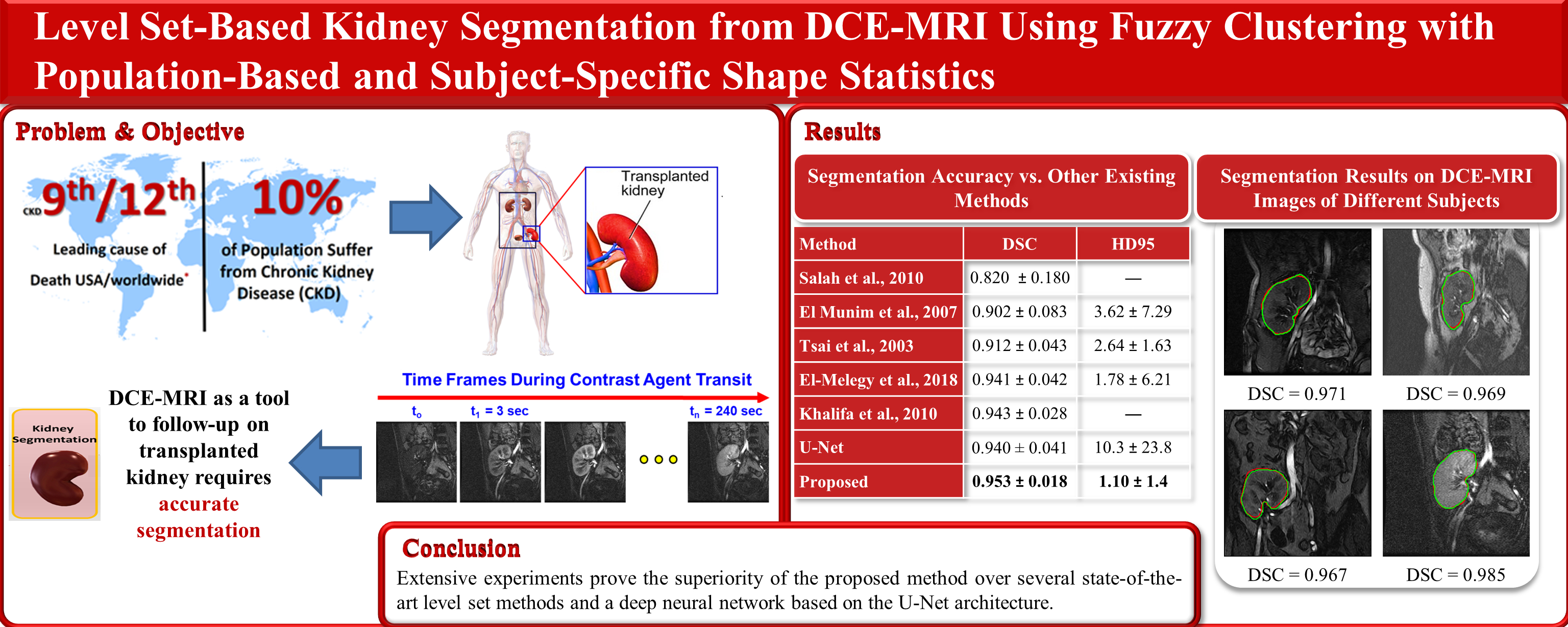
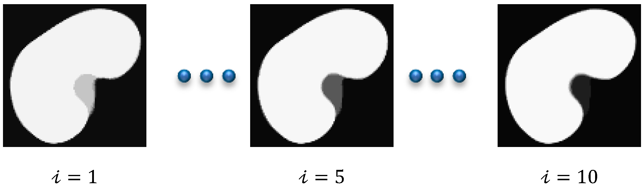
1]. In this respect, the DCE-MRI technique has achieved an increasingly important role in measuring the physiological parameters of the kidney and follow-up patients. DCE-MRI data acquisition is carried out through injecting the patient with a contrast agent and, during the perfusion, the kidney images are captured quickly and repeatedly at three second intervals. The contrast agent perfusion leads to contrast variation in the acquired images. Consequently, the intensity of the images at the beginning of the sequence is low (pre-contrast interval), gradually increases until reaching its maximum (post-contrast interval), and then decreases slowly (late-contrast interval).
Figure 1 shows a time sequence of DCE-MRI kidney images of one of the patients that was taken during the contrast agent perfusion. Accurate kidney segmentation from these images is an important first step for a complete noninvasive characterization of the renal status. However, segmenting the kidneys is challenging due to the motion that is made by the patient’s breathing, the contrast variation, and the low spatial resolution of DCE-MRI acquisitions [
1,
2].
In order to overcome these problems, several researchers have proposed multiple techniques to segment the kidney from DCE-MRI images. A careful examination of the related literature reveals that level-set-based segmentation methods [
3,
4,
5,
6,
7,
8] have been the most popular for this purpose. In these methods, a deformable model adapts to the shape of the kidney, its evolution being constrained by the image properties and prior knowledge of the expected kidney shape. In [
3], the authors developed a DCE-MRI kidney segmentation method employing prior kidney shape and gray-level distribution density in the level set speed function in order to constrain the evolution of the level set contour. However, their method had large segmentation errors on noisy and low-contrast images. Thus, in [
4,
5], Khalifa et al. proposed a speed function combining the intensity information, the shape prior information, and the spatial information modeled by 2nd- and 4th-order Markov Gibbs random field (MGRF) models, respectively. In order to circumvent the issue of the rather similar appearance between the kidney and the background tissues, Liu et al. [
6] proposed to remove the intensity information from the speed function in [
5] and to use a 5th-order MGRF to model the spatial information.
Incorporating the shape information into the level set method typically requires a separate registration step [
3,
4,
5,
6] to align an input DCE-MRI image to the shape prior model in order to compensate for the motion that is caused by the patient’s breathing and movement during data acquisition. In a different manner, Hodneland et al. [
7] proposed a new model that jointly combines the segmentation and registration into the level set’s energy function and applied it to segment kidneys from 4D DCE-MRI images.
From another perspective, the level set contour evolution is guided by deriving a partial differential equation in the direction that minimizes a predefined cost functional containing several weighting parameters that need manual tuning [
3,
4,
5,
6,
7]. In contrast, Eltanboly et al. [
8] proposed a level set segmentation method employing the gray-level intensity and shape information without using weighting parameters. Some work [
9,
10] has also been carried out in addressing the intensity inhomogeneity and the low contrast problems of DCE-MRI images that are caused during the acquisition process. Based on fractional calculus, Al-Shamasneh et al. [
9] proposed a local fractional entropy model to enhance the contrast of DCE-MRI images. Later, in [
10], they presented a fractional Mittag-Leffler energy function based on the Chan-Vese algorithm for segmenting the kidneys from low-contrast and degraded MR images.
More recently, convolutional neural networks (CNNs) have been successfully used for several image segmentation tasks, including kidney segmentation. For example, Lundervold et al. [
11] developed a CNN-based approach for segmenting kidneys from 3D DCE-MRI data using a transfer learning technique from a network that was trained for brain hippocampus segmentation. Haghighi et al. [
12] employed two cascaded U-Net models [
13] to segment kidneys from 4D DCE-MRI data. Later on, Milecki et al. [
14] developed a 3D unsupervised CNN-based approach for the same reason. Bevilacqua et al. [
15] presented two different CNN-based approaches for accurate kidney segmentation from MRI data. On the other hand, the authors in [
16] integrated a mono-objective genetic algorithm and deep learning for an MRI kidney segmentation task. Isensee et al. [
17] presented the top scoring model in the CHAOS challenge [
18] for an abdominal organs segmentation task, in which they used an nnU-Net model to segment the left and right kidneys from MRI data. The CHAOS challenge dataset includes the data of 80 different subjects, including 40 CTs and 40 MRIs. Each sequence contains an average of 90 scans in CT and 36 in MRI in the DICOM format.
The research gap is as follows: The common stumbling block facing CNN methods is that they typically require annotated data of a large size in order to train the network, which is often difficult to obtain in the medical field. Thus, the aforementioned deep learning methods struggle to achieve high segmentation accuracy. On the other hand, the level-set-based kidney segmentation methods [
3,
4,
5,
6,
7,
8] have proved their effectiveness in achieving a superior performance with more accurate segmentation. However, unfortunately, almost all of them need accurate level set contour initialization to be performed manually by the user. Inaccurate initialization may cause a drop in the segmentation accuracy or even cause the method to fail. In order to overcome this problem, in [
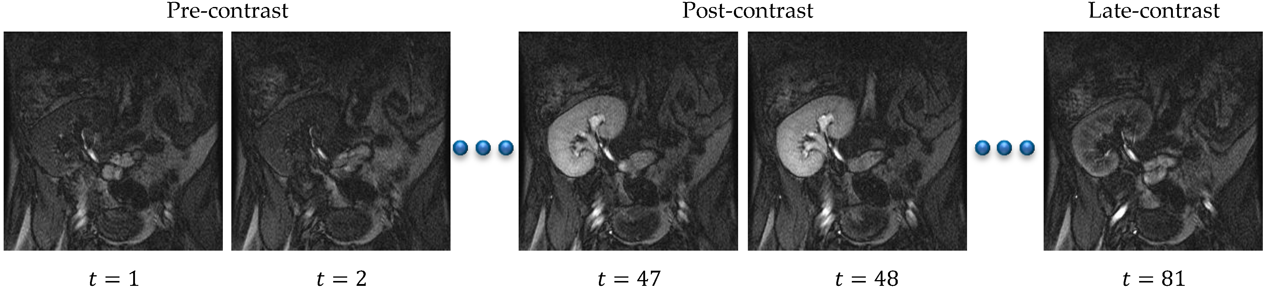
19] we have presented an automated DCE-MRI kidney segmentation, called FCMLS, based on FCM clustering [
20] and level sets [
21]. In our FCMLS method, we constrain the contour evolution by the shape prior information and the intensity information that are represented in the fuzzy memberships. In addition, in order to ensure the robustness of the FCMLS method against contour initialization, we employ smeared-out Heaviside and Dirac delta functions in the level set method. The FCMLS method has indeed demonstrated its efficiency in segmenting the kidneys from DCE-MRI images. However, it still has some limitations. First, its performance drops on low-contrast images, such as those in the pre- and late-contrast parts of the time sequence in
Figure 1. Second, the FCM algorithm is used for computing the fuzzy memberships of the image pixels before the level set evolution begins. Once the level set starts evolving, the obtained memberships are not changed, and this might be not accurate enough in some cases.
In order to enhance the segmentation accuracy of FCMLS, and to improve its robustness on low-contrast images, we have developed a new kidney segmentation method, named the FML method, in [
22]. In this method, we model the correlation between neighboring pixels into the level set’s objective functional by a Markov random field energy term. We also embed the FCM algorithm into the level set method and iteratively update the fuzzy memberships of the image pixels during contour evolution. The experimental results have confirmed the improved accuracy and robustness of this method. However, the integration of the Markov random field model within the level set formulation has increased the computational complexity of the FML method significantly.
In this paper, we follow a different strategy in order to improve the segmentation performance of our previous method without sacrificing the computational complexity. The shape information plays a key role in kidney segmentation since human kidneys tend to have a common shape, with between-subject variations. Thus, we seek to take full advantage of this in our new level set formulation by exploiting the level set method’s flexibility to accommodate the shape information about the target object that is to be segmented [
23]. Inspired by [
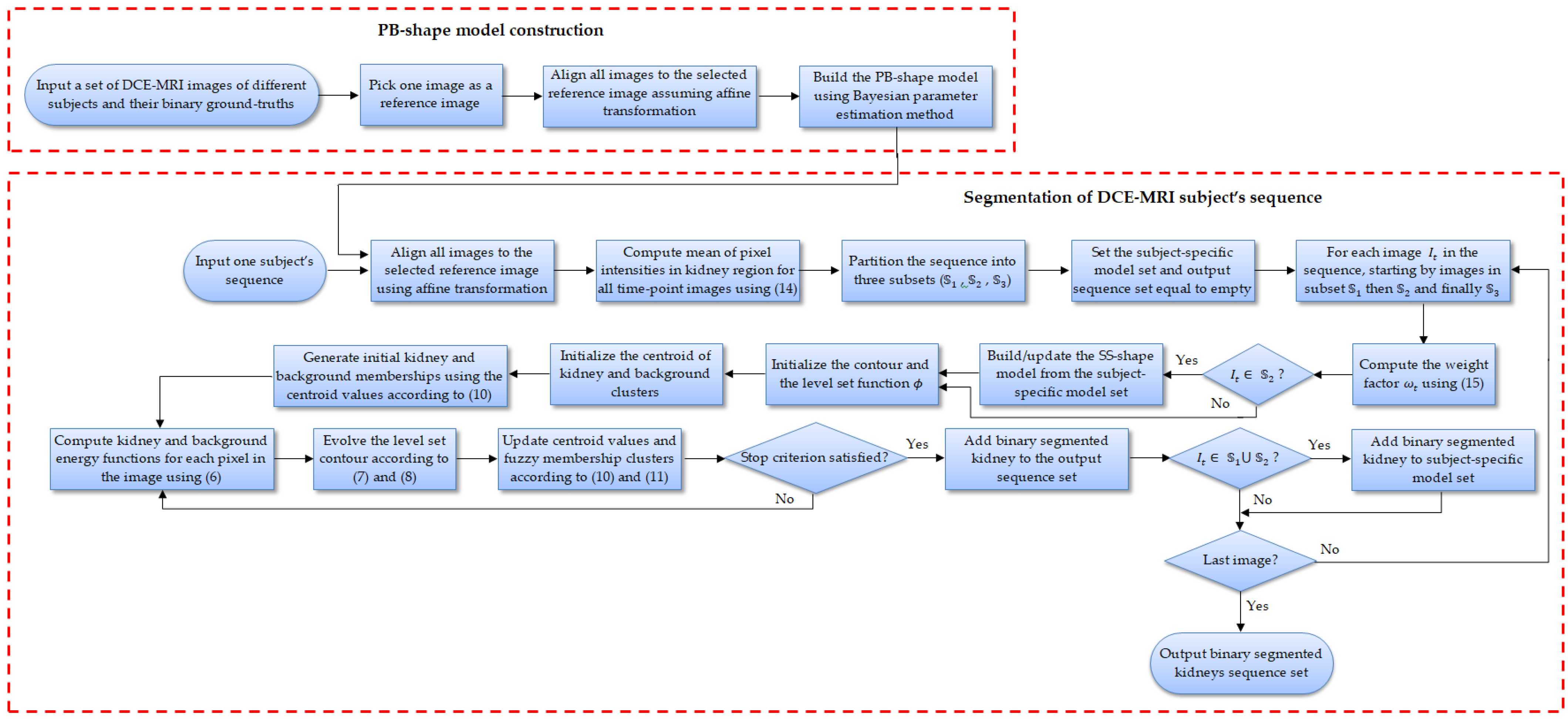
24], we employ PB-shape and SS-shape models for kidney segmentation. The PB-shape model is built offline from a range of kidney images from various subjects that are manually segmented by human experts, whereas the SS-shape model is constructed on the fly from the segmented kidneys of a specific patient.
This new methodology is able to generate high segmentation accuracy because the PB-shape model is used on images with high contrast in the post-contrast interval of the image sequence. Moreover, the SS-shape model that is generated from those accurate segmentations is employed on the more challenging, lower contrast images from pre- and late-contrast intervals of the sequence, as it more accurately reflects the kidney’s shape from the same patient. Our early work on this new methodology has been drafted in [
25], on which we build and develop several novel contributions in the present paper. First, we embed FCM clustering into the level set evolution. Thus, the kidney/background fuzzy memberships are computed and updated every time the level set contour evolves. Second, the representation of the shape information in [
25] is based on a 1st-order shape method, which might be inaccurate when some kidney pixels are not observed at all in the images that are used to construct the shape model. In this paper, we adopt an efficient Bayesian parameter estimation method [
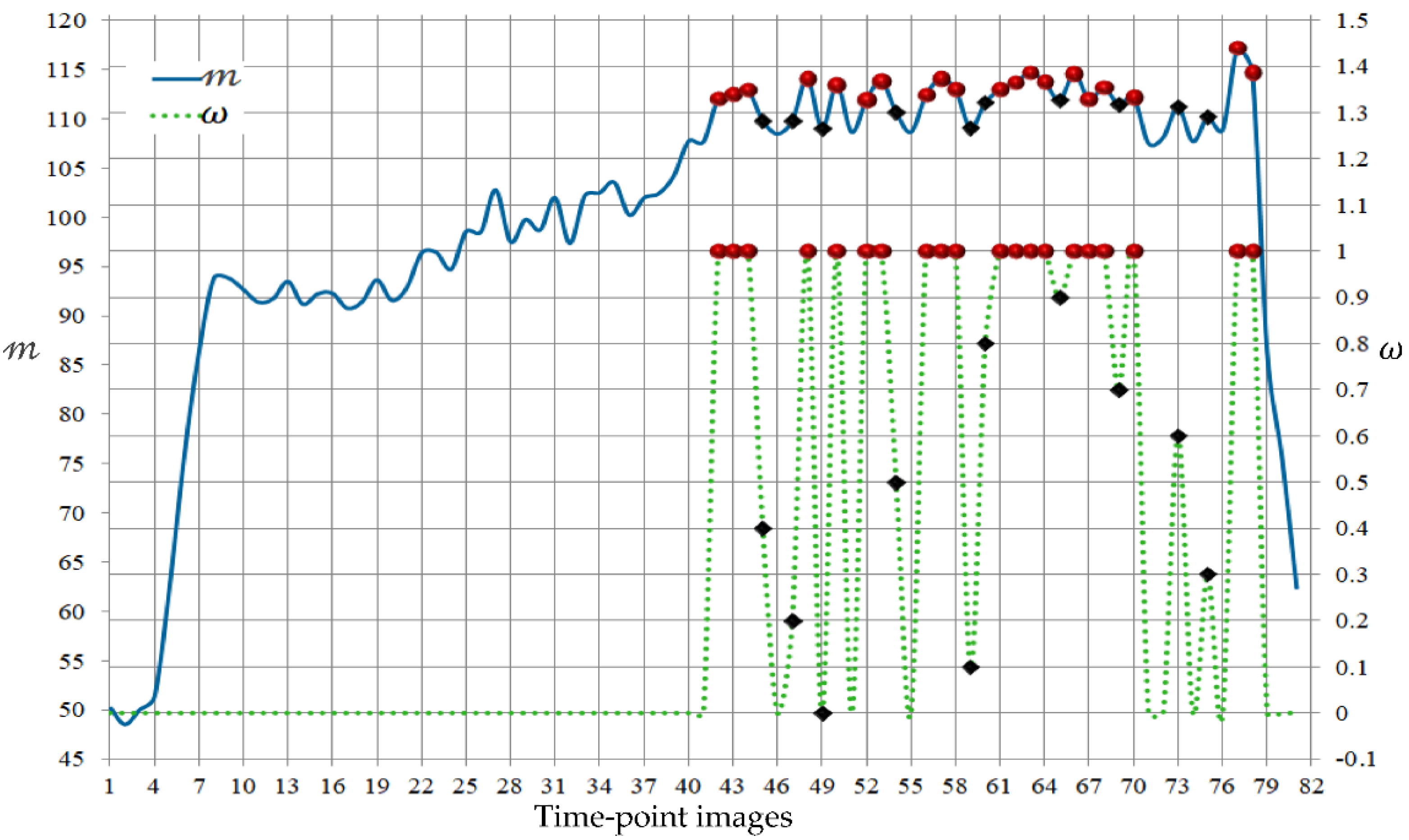
26] in computing the PB-shape and SS-shape models, which more accurately accounts for the kidney pixels that are possibly not observed during the model building. Third, we propose an automated and time-efficient, yet effective, strategy to determine the images from the patient’s sequence, to which the PB-shape model, the SS-shape model, or both of the models blended together are applied.
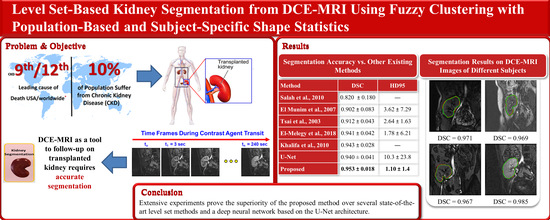
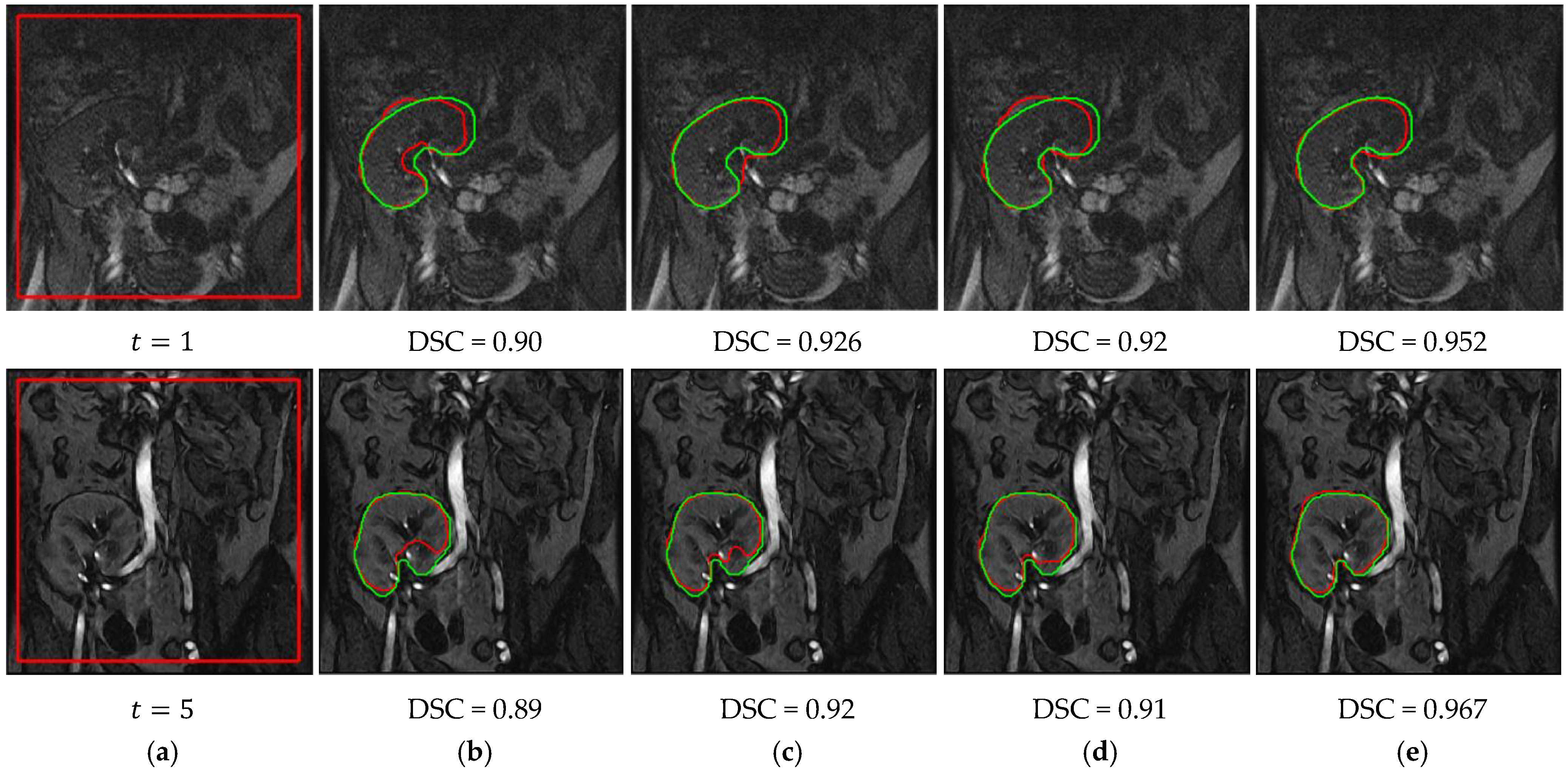
The proposed method is used to segment the kidneys of 45 subjects from DCE-MRI sequences, and the segmentation accuracy is assessed using the Dice similarity coefficient (DSC), the intersection-over-union (IoU), and the 95-percentile of Hausdorff distance (HD95) metrics [
2,
27]. Our experimental results prove that the proposed method can achieve high accuracy, even on noisy and low-contrast images, with no need for tuning the weighting parameters. The experiments also show that the segmentation accuracy is not affected by changing the position of the initial level set contour, which demonstrates the high consistency of the proposed method. We compare our method’s segmentation accuracy with several state-of-the-art level set methods, as well as our own earlier methods [
19,
22,
25]. Furthermore, we compare its performance against the base U-Net model and one of its modifications named BCDU-Net [
28], which is trained for the same kidney segmentation task. The two networks are trained from scratch on our DCE-MRI data, which are augmented with the KiTS19 challenge dataset [
29]. This dataset contains 300 subjects’ data, where 210 out of all of the data are publicly released for training and the remaining 90 subjects are held out for testing. Each subject has a sequence of high quality CT scans, with their ground-truth labels that are manually segmented by medical students. It also includes a chart review that illustrates all of the relevant clinical information about this patient. All of the CT images and segmented annotations are provided in an anonymized NIFTI format. The comparison results confirm that the proposed method outperforms all of the other methods.
The remainder of this paper is structured as follows:
Section 2 introduces the mathematical formulation of the proposed kidney segmentation method. Then,
Section 3 provides the experimental results and the comparisons. Finally, a discussion and the conclusions are presented in
Section 4.


 ,
, 


