Internationalization in the Baltic Regional Accounts: A NUTS 3 Region Dataset

Abstract

Features of internationalization, such as trade, foreign direct investments, and international migration, are crucial for understanding the economic developments of small and open economies. However, studying internationalization at the country level may obscure significant heterogeneity in its relationship with economic growth and other economic and social outcomes. Regional accounts provide insights into the geography of internationalization, but collections of such disaggregated statistics are rarely provided by statistical bureaus. The purpose of this paper is twofold. First, we demonstrate how regional account data, including internationalization indicators, can be constructed to obtain consistent and homogeneous regional-level series using a combination of micro and macro data sources. Second, our aim is to foster spatial research on internationalization and the spatial economy in the Baltics by providing comprehensive data collection of socio-economic variables at the NUTS 3 regional level over time. This collection encompasses trade, FDI, and migration, enabling the study of internationalization and other features of the Baltic economy. We present a series of key features, revealing noticeable correlation patterns between regional development and internationalization.

Dataset: https://zenodo.org/records/10223416.

Dataset License: CC-BY

1. Summary

Internationalization plays an essential role in the economic development of open economies, but the spatial dimensions within each economy are less frequently assessed. Regional accounts may shed light on the domestic geographies of internationalization. Yet, they are often inaccessible and seldom contain internationalization variables. Despite the significant economic growth and regional internationalization over the last decades, few spatial studies on internationalization stand out for the Baltic states. Simultaneously, regional internationalization data, such as trade and foreign investment data, remain scarce [1].

This paper has two objectives. First, we aim to demonstrate how regional account data, including internationalization indicators, can be processed and analyzed through descriptive statistics and by providing a dataset suitable for further investigations. We pay particular attention to internationalization proxies, including trade, foreign direct investments, and migration, as these variables are typically less available in regional accounts.

In our facilitation of studies on internationalization across the Baltic regions, we provide descriptive statistics and a dataset containing the Baltic regional accounts. We reveal some key correlation patterns concerning regional development and internationalization through descriptive statistics. Our objective here is not to determine the causality of the linkages but rather to identify patterns worthy of further investigation. Moreover, causal links may run in various directions, and many cofounders may come into play.

We document the collection and processing of internationalization variables. In our dataset, internationalization is represented by trade (i.e., export and imports), foreign direct investments (FDI) in equity stocks (both outgoing and incoming), and international migration (i.e., emigration and immigration). Among these, trade and migration constitute flows, while the changes in the FDI stocks correspond to the sum of FDI flows, excluding dividends and revaluation after dividends.

Moreover, the collected and processed dataset includes a wide range of variables. The data are sourced from various providers, with domestic firm data, Eurostat, Global Data Hub, and OECD being the most commonly used sources. To ensure comparability across countries, the variables are harmonized across international sources. Additionally, we utilize alternative sets of deflators to obtain fixed-price figures. For recent years, migration data were available, but adjustments to figures related to population changes have been necessary to achieve a more accurate representation. The collection and processing of this dataset are documented in this study, illustrating how such datasets may be collected.

Our contributions to domestic variables are mostly limited to data collection, data harmonization, handling of measurement errors, and filling out data gaps. Yet, some contributions to the processing of domestic data are worth mentioning explicitly here. Most notably, we estimate the fixed capital stock for all three countries, exploiting a combination of firm-level data and macro data.

In a regional account setting, the appearance of the fixed capital stock variable resembles FDI and trade variables somewhat in the sense that it is seldom reported but could be approximated by the help of firm data and macro data. Furthermore, our collection of deflators also allows for the calculation of volume figures.

At last, we pinpoint that the harmonization of some data series required more extensive processing than others. For the Estonian population data, we adjust for a data break between 2014 and 2015 in the years prior to 2015, such that the population figures for this period are comparable with the population figures in the sequent period. To address measurement errors in survey-based broadband data, we assume that broadband coverage cannot decrease and replace extreme outliers with their interpolated values.

The descriptive statistics presented in this paper depict close linkages between internationalization and economic development in many instances, but the correlation patterns are not always strong. It is interesting to see that Estonia’s position as the most advanced Baltic economy is largely due to the dominant role of the capital region of Põhja-Eesti. Along the center-periphery, the Baltic NUTS 3 regions (i.e., regions at the third level of Eurostat’s nomenclature of territorial units for statistics) resemble each other across countries in many respects. Regarding overall economic activities, internationalization is more pronounced in most urban regions. Exports and international immigration involve the most considerable exceptions from this pattern, Telšiai and Klaipėda being the most exporting Baltic regions per employment and Šiauliai being the Baltic region with the highest international immigration per capita. Overall, FDI and trade tend to be highly correlated with the indicators of economic performance, human development, and knowledge generation, whereas the correlations between migration and the same indicators, for the most part, are weaker.

To help facilitate further research on internationalization and other features of the Baltic spatial economy, a dataset with the regional Baltic accounts at the NUTS 3 level, inter alia including internationalization variables, accompanies this paper as Supplementary Materials. By exploiting a combination of firm-level data and macro data on FDI, trade, and fixed capital, we are able to approximate these variables across the Baltic regions.

Our methodological demonstration exemplifies how different data possibilities call for different data collection and processing methodologies. While some data at the regional level can be collected from macro sources or estimated from micro sources, others must be approximated by a combination of variables from various data sources. To ensure comparability across countries, we have harmonized the collected figures with corresponding figures in macro statistics.

Admittedly, approximation of variables and missing or unreliable observations will never be of similar quality as the true data. While some approximations were made, the data are still expected to be of relatively high quality. As long as the measurement errors in approximated elements are not systematically biased in the same direction, they will only add noise to the analysis. More data collection and processing resources can always contribute to higher data quality. Still, our data handling illustrates how decent data quality can be achieved with reasonable effort. Overall, we believe that our dataset is both suited for achieving a good overview of key socio-economic conditions in the Baltic region and for further econometric investigations into key relationships.

For future research, we hope for more studies on internationalization and the spatial economy, particularly in the Baltics and with the help of our dataset. We also welcome more contributions on how regional accounts data can easily be collected and processed.

2. Data Description

In this section, we document the content of our Baltic regional accounts. All variables cover at least 2007 to 2015 and mostly up to 2019, but some variables cover a longer period from 1991 to 2020.

We start by presenting the Baltic NUTS 3 regions and applying the industry classification. Then, we move on to documentation of the data content, listing each relevant variable.

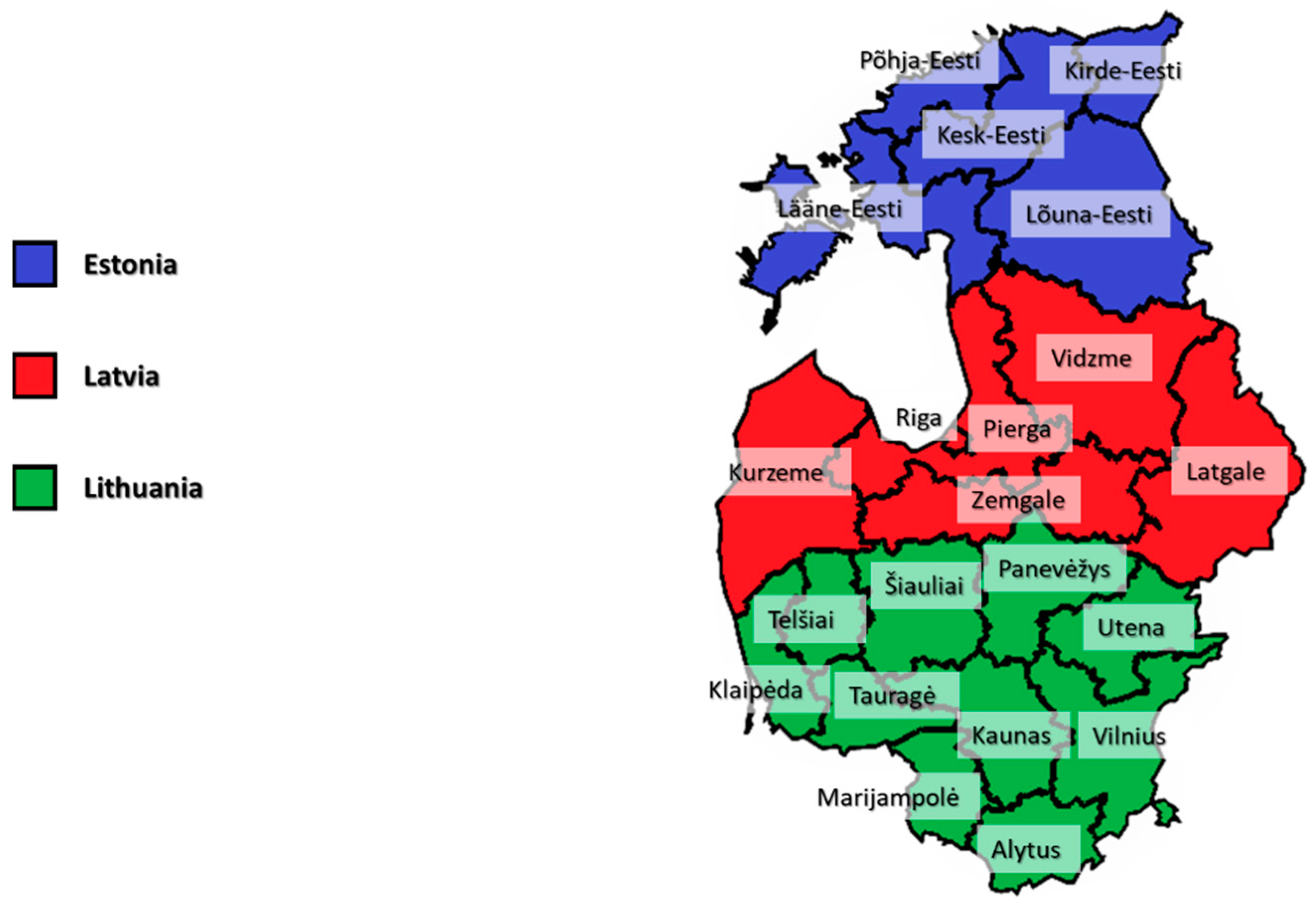
2.1. Classifications for Regions and Industries

The Baltic countries contain 21 NUTS 3 regions, distributed over 11 in Lithuania, 6 in Latvia, and 5 in Estonia. In Figure 1, we provide a map of the Baltic NUTS regions, which lies as the foundation for our mapping.

In our study, we process data using Eurostat and OECD’s industry classification applied to the regional statistics. This classification involves 11 industries and is rendered in

Table 1. Industry classification.

Industry Name	Industry Codes
Primary industries	NACE 1 to 3
Manufacturing	NACE 10 to 33
Other resource industries	NACE 5 to 9 and NACE 35 to 39
Construction	NACE 41 to 43
Trade, transportation and tourism	NACE 45 to 56
Information and communication	NACE 58 to 63
Finance	NACE 64 to 66
Real estate	NACE 68
Knowledge-intensive business services and business support	NACE 69 to 74
Public services	NACE 84 to 89
Household and non-profit services	NACE 90 to 99

. In addition to reporting employment and gross value added in basic prices with affiliated deflators for each industry, we exploit the industry classification in the running account estimation of some variables (i.e., outgoing FDI, exports, imports, and fixed capital).

2.2. Content of the Dataset

The content of our Baltic regional account dataset is listed in

Table 2. Overview of variables in the dataset for the Baltic regional accounts.

Variable	Measurement
International emigration and immigration in terms of people migrating	Measured in number of people from 2006 to 2019
Exports and imports in current and fixed 2010 prices, deflated with national price indexes for exports and imports, respectively	Measured in Million euros from 2007 to 2019
Outgoing foreign direct investments in equity stocks, including reinvestments of earnings, measured in current prices and fixed 2010 prices, deflated with price indexes for the domestic product or total end use at the national or European Union level	Measured in Million euros from 2006 to 2019
Incoming foreign direct investments in equity stocks, including reinvestments of earnings in current prices and fixed 2010 prices, deflated with price indexes for either the domestic product or total end use at the national or European Union level	Measured in Million euros from 2007 to 2019
Gross value added in basic prices deflators with 2010 as the base year, measured for 11 industries and at the national level	Measured in the percentage of 2010 prices from 2000 to 2018 at regional and industry levels, and from 2000 to 2019 at the national level
Gross value added in market prices deflator at the national level with 2010 as the base year	Measured in the percentage of 2010 prices from 2000 to 2019
Fixed capital deflator with 2010 as the base year
End-use deflators with 2010 as the base year, including deflators for total end use (sum of consumption, exports, and gross investments in inventories and fixed capital), and total and household consumption
Trade deflators for exports and imports with 2010 as the base year, measured at national and EU-27 levels
Total income deflator with 2010 as the base year	Measured in the percentage of average EU-27-2020 prices from 1995 to 2020
Purchasing power parity for production and consumption with EU-27 of 2020 as a basis	Measured in purchasing power parity of EU-27 in 2020
Exchange rate between Euro and US Dollar	Measured in Euros per US Dollars from 2000 to 2020.
Gross value added measured at basic prices, reported for 11 industries in current prices and fixed 2010 prices	Measured in Million euros from 2000 to 2019
Gross value added measured at market prices, reported in current prices
Net product taxes, reported in current prices
Employment mid-year reported for all ages with further split into employment relationship (i.e., employees and self-employed) and 11 industries, 15 to 64 years old divided into genders, 15 to 24 years old, 25 to 64 years old, and more than 65 years old	Measured in the number of people from 1999 to 2019 in general and 2000 to 2019 for figures concerning industry affiliation or employment relationship
Unemployment mid-year, reported for either gender or the age groups 15 to 24 years old and 25 to 64 years old, with further disaggregation into short-term and long-term unemployed people (i.e., unemployed for less and more than a year, respectively)	Measured in the number of people from 1999 to 2019
Rate of young people not in employment, education or training, age 18 to 24 years old	Measured from 2005 to 2017
Rate of early leavers from education and training, age 18 to 24 years old	Measured in population share from 2002 to 2017
Gross fixed capital stock at the end of each year, reported in current prices and fixed 2010 prices	Measured in Million euros from 2000 to 2019
Patent Cooperation Treaty patent applications are fractional counted by residence, total co-count by workplace and fractional count by workplace, where the latter count is further disaggregated into biotechnical, ICT-related, medical, nano-scientific, and pharmaceutical patent applications.	Measured in the number of property rights from 1991 to 2015
Community designs, applications, activated and registered unitary industrial design rights	Measured in the number of property rights from 2003 to 2016
European Union trademarks, applications and registered trademarks	Measured in the number of property rights from 1996 to 2016
Latent broadband access coverage for households, defined as the portion that subscribes to an internet connection of at least one Megabit per second	Measured in the share of households from 2004 to 2019
Population at the beginning of the year, divided into gender and five-year age groups from 0 to 4 years to 80 years and above, as well as population between 25 and 64 years with primary and lower secondary education, higher secondary and vocational education, and tertiary education	Measured in the number of people from 1995 to 2020 in general with a shorter time span of 2000 to 2018, when the population is distributed across education types
Natural population growth, divided into births and deaths	Measured in the number of people from 1995 to 2020
Domestic migration, disaggregated into domestic immigration and domestic emigration	Measured in the number of people from 2006 to 2019
Life expectancy at birth	Measured in the number of years from 1995 to 2019
Infant mortality, measured as deaths in the first year of life	Measured in the number of fatalities from 2002 to 2019
Transportation-related mortality, measured as deaths in traffic	Measured in the number of fatalities from 2005 to 2018
Intentional homicides at year of death	Measured in the number of units from 2005 to 2017
Human development index, divided into subindexes for education, health, and income	Measured in the percentage of hypothetical optimal score from 1995 to 2019
Years of schooling in mean for completed education and in expectation upon entering education.	Measured in the number of years score from 1995 to 2019
Disposable household income measured in current prices, fixed 2010 prices, and purchasing power parities with European Union-27-2020 as a basis	Measured in Million euros from 2004 to 2018.
Gross national income in current prices, fixed 2010 prices and purchasing power parities with European Union-27-2020 as a basis	Measured in Million euros from 2000 to 2019
Active physicians, including practicing physicians and other physicians for whom the execution of their job requires medical education	Measured in the number of units from 2005 to 2017
Hospital beds, including acute care beds, rehabilitative care beds, long-term care beds, and other beds in hospitals
Area measured in square kilometers, divided by land area and freshwater area	Measured in square kilometers from 1991 to 2020
Main rooms in dwellings, including bedrooms and living rooms	Measured in the number of rooms from 2005 to 2017
Degree days in terms of cooling degree days and heating degree days	Measured in index points from 1995 to 2020

, including indications of measurement. Note that the internationalization figures and fixed capital are the most processed and estimated among the variables. The other variables can largely be collected from other statistical sources, although some data cleaning will be required. Further details about each variable of the dataset are provided in the metadata of the dataset.

3. Methods

In this section, we document our collection and processing of data for the Baltic regions. As data access varies, different collection and processing methodologies for each country are applied for some variables. We start by devoting our attention to the internationalization variables, as the data processing required for collecting these variables is relatively extensive. Then, we move on to domestic variables. In Appendix A, we provide technical notes on the estimation of variables missing at the regional level and on data cleaning.

3.1. Collection and Processing of Internationalization Variables

In this subsection, we document the collection and processing of internationalization variables. The internationalization variables in the Baltic regional accounts, presented in this paper, include trade (i.e., export and imports), FDI in equity stocks (both outgoing and incoming), and international migration (i.e., emigration and immigration). Among these, trade and migration are reported as flow variables, while FDI is reported as stocks. The FDI stocks correspond to the sum of FDI flows, excluding dividends and revaluation after dividends. When applied in the running calculation, trade and FDI figures are reported in USD and international data sources are converted to EUR using the annual exchange rates obtained from the central bank of Norway.

The collection and processing of international migration data are summarized at the top of

Table 3. Data collection and processing of global migration, international trade, and foreign direct investment figures over countries.

Country	Data Collection and Processing
International emigration and immigration
Measured in number of people from 2006 to 2019
Estonia	International emigration and immigration figures at the regional level are obtained from Statistics Estonia. Unexplained population growth is ascribed to international immigration and emigration, when it is positive and negative, respectively. We make an exception for a data break between 2014 and 2015, where many people are moved in the registers from one region to another. We approximate this error by the national average of the positive and negative residuals in absolute value multiplied by the regional share of the residual with the same sign.
Latvia	International emigration and immigration figures at the regional level are obtained from the Official Statistics of Latvia for 2010 to 2018. For 2007 and 2010 only, we assume that the regional shares of both emigration and immigration correspond to the absolute regional value of population change divided by the total value of population change. Unexplained population growth is ascribed to international immigration when it is positive and international emigration when it is negative.
Lithuania	International emigration and immigration figures at the regional level are obtained from Statistics Lithuania. We ascribe unexplained population growth to international immigration or emigration, depending on whether the sign is positive or negative, respectively.
Exports and imports
Current and fixed 2010 prices, deflated with national price indexes for exports and imports, respectively. Measured in Million euros from 2007 to 2019
Estonia	We approximate the regional distribution of exports and imports with trade figures from the Statistic Estonia firm-market-product level commodity trade data based on customs statistics and firm-level services trade data from the Bank of Estonia. Regional trade is scaled annually to ensure that the aggregate trade figures match the national figures reported by the WTO for each year.
Latvia	We approximate the regional distribution of commodity trade with trade figures in firm data from the Central Statistical Bureau of Latvia’s ‘Complete report on activities’. For service trade, we assume that the distribution of regional trade is the same on an annual basis per gross value added within the relevant industries, recognized as construction and service industries, excluding wholesale and retail trade. Service trade figures are not available at the micro level. We obtain each industry’s service trade at the national level from OECD’s annual input–output matrixes for transactions between Latvian industries and sectors, enabling us to estimate regional figures. Commodity trade and service trade are scaled separately on an annual basis to match the aggregate trade figures of the WTO, before being aggregated.
Lithuania	Regional direct export and national re-export are collected from Statistics Lithuania. To obtain total export figures for each region, we assume that the re-export follows the same regional distribution as the direct export. However, Statistics Lithuania only reports national import figures. To overcome this challenge, we assume that the distribution of regional imports is the same per gross value added within each industry and year. We obtain each industry’s import at the national level from OECD’s annual input–output matrixes for transactions between Lithuanian industries and sectors, enabling us to estimate regional imports. Regional trade is scaled to match the aggregate trade figures reported by the WTO annually.
Incoming foreign direct investments
Equity stocks, including reinvestments of earnings in current prices and fixed 2010 prices, deflated with price indexes for either the domestic product or total end use at the national or European Union level. Measured in Million euros from 2007 to 2019
Estonia	We approximate the regional distribution of incoming FDI with FDI figures in the enterprise register data. The regional incoming FDIs are scaled annually such that the aggregate incoming foreign direct investments are equal to the national figures reported by the IMF from 2009. The IMF series are extrapolated backwards to 2007 based on the developments in similar series from OECD.
Latvia	We approximate the regional distribution of incoming FDI with the help of the Central Statistical Bureau of Latvia’s ‘complete report on activities’ and firm financial data provided by the State Revenue Service of the Republic of Latvia, proxying the weights by the product between equity and a dummy indicating incoming FDI. The regional incoming FDIs are scaled annually such that aggregate exports are equal to the national figures reported by IMF from 2009. The IMF series are extrapolated backwards to 2007 based on the developments in similar series from OECD.
Lithuania	Regional figures for incoming FDI are obtained from Statistics Lithuania. The FDI figures are scaled, such that the aggregate figures match the figures reported by IMF from 2009. The IMF series are extrapolated backwards to 2007 based on the developments in similar series from OECD.
Outgoing foreign direct investments
Equity stocks, including reinvestments of earnings in current prices and fixed 2010 prices, deflated with price indexes for the domestic product or total end use at the national or European Union level. Measured in Million euros from 2006 to 2019
Estonia	We approximate the regional distribution of outgoing FDI with the help of enterprise register data and the Bank of Estonia’s firm-level outward FDI data, proxying the weights by the product between total assets and a dummy indicating outgoing FDI. The outgoing regional FDIs are scaled annually such that aggregate outgoing FDI is equal to the national figures reported by IMF from 2009. The IMF series are extrapolated backwards to 2007 based on the developments in similar series from OECD.
Latvia	We approximate the regional distribution of outgoing FDI with the help of the Central Statistical Bureau of Latvia’s ‘complete report on activities and firm financial data provided by the State Revenue Service of the Republic of Latvia, applying two equally weighted proxies for the magnitude of each investment. These are total assets in subsidiaries and the product between total assets in subsidiaries and a dummy indicating outgoing FDI. The regional outgoing FDIs are scaled annually such that aggregate figures are equal to the national figures reported by the IMF from 2009. The IMF series are extrapolated backwards to 2007 based on the developments in similar series from OECD.
Lithuania	Statistics Lithuania only report national outgoing FDI figures. To overcome this challenge, we assume that the distribution of regional outgoing FDI is the same per gross value added within each industry and year. We obtain each industry’s outgoing FDI at the national level from OECD’s FDI statistics, enabling us to estimate regional imports. At last, the FDI figures are scaled, such that the aggregate figures match the figures reported by IMF in 2009. The IMF series are extrapolated backwards to 2007 based on the developments in similar series from OECD.

. For all countries, registered figures for emigration and immigration can be collected from the national statistical bureaus, except for Latvia, from 2007 to 2010. In the latter case, the statistics are approximated based on the regional distribution of net migration in absolute values and national figures for international migration.

Population changes can be divided into natural population growth, domestic migration, and international migration. Except for a data break in Estonia in 2014, unexplained population growth using this equation is ascribed to global immigration. This choice is made as positive residuals tend to be correlated with the European migration flows (e.g., the Syrian refugee crisis and Brexit), and international refugee flows and working migration back and forth tend to occasionally be unregistered.

Further down in the table, we provide an overview of the compilation and processing of trade figures. For Estonia’s total trade and Latvian commodity trade, we exploit firm-level data to estimate the distribution of exports and imports across regions, including both commodity and service trade. For Lithuania overall and Latvian service trade, regional statistics for direct export are used to proxy the regional distribution of total export. At the same time, industry-specific gross value added is exploited for industry-specific shares for total imports. To ensure comparability across countries, all trade figures are harmonized against the national statistics reported by the World Trade Organization (WTO).

We estimate incoming foreign direct investment (FDI) equity stocks for the Baltic regions by a wide range of approaches, as listed further in the notes below the table. For each country, the approach depends on the data availability. All FDI figures are harmonized with national statistics reported by the International Monetary Fund (IMF), which is extended by data from the Organization for Economic Co-operation and Development (OECD) to ensure comparability across countries.

We use firm-level data to proxy the regional distribution of FDI for Estonia and Latvia. For incoming FDI, the Estonian firm data include actual incoming FDI, making the regional distribution straightforward to estimate. For Latvia, we proxy the regional distribution by the product between a dummy for incoming FDI and the equity value. While the latter approach results naturally in less precise figures on FDI statistics, investigations of the Estonian data—which include complete ownership statistics—suggest that it is probably not a major issue. Moreover, most Estonian companies subject to FDI have relatively high foreign ownership shares, which seldom are below 50 percent.

Country-specific data collection approaches are also used for outgoing FDI, conferring at the bottom of Table 3. For outgoing FDI from Estonia, we apply the product between a dummy for outgoing FDI and the value of assets in subsidiaries as regional weights. We have the same possibility for Latvia, but here the data for the outgoing FDI dummy are considerably incomplete in terms of coverage. Accordingly, we use the value of assets in subsidiaries for all firms as a second proxy for the Latvian regional distribution of outgoing FDI. When approximating the regional distribution of the outgoing Latvian FDI, we put equal weight on the two proxies.

In the case of Lithuania, regional figures for incoming FDI are provided by Statistics Lithuania. For outgoing Lithuanian FDI, we combine industry-specific investment intensities from the OECD and the regional distribution of gross value added per industry to approximate the regional distribution.

3.2. Collection and Processing of Domestic Variables

In this subsection, we turn to the collection and processing of domestic variables. We will provide an overview of the primary processes involved in collecting and processing data, while measures to deal with particular issues with incomplete data are accounted for in Appendix B.

We start by presenting fixed capital figures. These figures are not directly accessible at the regional level from statistical sources and thus have to be estimated, as explained in detail in

Table 4. Data collection and processing of fixed capital stock.

Fixed Capital Stock
Gross stocks at the end of each year, reported in current prices and fixed 2010 prices. Measured in Million euros from 2000 to 2019.
Estonia	The gross fixed capital stocks in the current price are estimated from 2007 to 2019 as the sum of tangible and intangible fixed capital stock based on enterprise register data. We extend the time series further backwards to 2000 based on data from Eurostat, assuming that the development in fixed capital stock corresponds to the development in the quasi-stocks of fixed capital. These quasi-stocks are estimated assuming that the fixed capital per gross value added in current prices is the same by industry across the country for each of the 11 industries in our study. Figures are harmonized with the aggregate fixed capital stock figures at Eurostat. We calculate the gross fixed capital stock in fixed prices as the ratio between the fixed capital in current prices and the aggregate fixed capital deflator.
Latvia	The gross fixed capital stocks in the current price are estimated from 2007 to 2019 as the sum of tangible and intangible fixed capital stock based on data from the State Revenue Service of the Republic of Latvia. We extend the time series further backwards to 2000 based on data from Eurostat, assuming that the development in fixed capital stock corresponds to the development in quasi-stocks of fixed capital. These quasi-stocks are estimated assuming that the fixed capital per gross value added in current prices is the same by industry across the country for each of the 11 industries in our study. Figures are harmonized with the aggregate fixed capital stock figures at Eurostat. We calculate the gross fixed capital stock in fixed prices as the ratio between the fixed capital in current prices and the aggregate fixed capital deflator.
Lithuania	We estimate the regional distribution of fixed capital stock in Lithuania by applying and then taking the average of two alternative approaches from 2007 to 2019. First, we collect figures for gross investments in fixed capital at the regional level from Statistics Lithuania with data for three years before the initial year of our time series. We convert the gross investment figures to fixed price figures with the help of the fixed capital deflator. Next, we calculate quasi-stocks for fixed capital by summing the depreciated gross investments and applying linear depreciation with a rate of 25 percent. We let the fixed capital stocks reported at Eurostat correspond to the national aggregates and exploit the quasi stocks to proxy the regional distribution of fixed capital. Second, we collect the fixed capital stocks in current prices for the 11 industries in our study from Eurostat and distribute them across regions, assuming that the fixed capital per gross value added in current prices is the same by industry across the country. In the period from 2000 to 2006, we only apply the latter-mentioned approach, as regional investment series are unavailable. Figures are harmonized with the aggregate fixed capital stock figures at Eurostat. Volume figures are obtained by dividing the fixed capital stock in current prices by the fixed capital deflator.

. For Estonia and Latvia, the regional distribution of fixed capital was approximated with the help of firm-level data from 2007 to 2019.

In the same period, we have applied equally weighted proxies for Lithuania to approximate the regional distribution. First, we have exploited Statistics Lithuania’s regional series for gross investments. Second, we have combined industry-specific regional distribution of gross value with industry-specific ratios between fixed capital stock and gross value added at the national level. For all three countries, we have extrapolated the development in fixed capital back to 2000, again combining industry-specific regional distribution of gross value with industry-specific ratios between fixed capital stock and gross value added at the national level. Furthermore, the aggregate fixed capital deflator was used for deflation purposes, and the figures were harmonized with the aggregate fixed capital stock figures at Eurostat. At last, we collect the fixed capital stocks in current prices for the 11 industries in our study from Eurostat and distribute them across the regions, assuming that the fixed capital per gross value added in current prices is the same by industry across the country.

In

Table 5. Data collection and processing of domestic variables on labor participation, price indexes, value added, information production and sharing, demographics, the population’s well-being, and physical settlement features.

Variable	Data Collection and Processing
Labor participation
Employment mid-year reported for all ages with further split into employment relationship (i.e., employees and self-employed people) and 11 industries, 15 to 64 years old divided into genders, 15 to 24 years old, 25 to 64 years old, and more than 65 years old	Overall figures, as well as figures for industry affiliation and employment relationship, are obtained from Eurostat’s regional statistics. In addition, the age distribution is obtained from OECD’s regional statistics
Unemployment mid-year, reported for either gender or the age groups 15 to 24 years old and 25 to 64 years old, with further disaggregation into short-term and long-term unemployed people (i.e., unemployed for less and more than a year, respectively)	Obtained from OECD’s regional statistics
Rate of young people not in employment, education or training, age 18 to 24 years old
Rate of early leavers from education and training, age 18 to 24 years old
Price indexes
Gross value added in basic prices deflators with 2010 as the base year, measured for 11 industries and at the national level	Industry-specific gross value added deflators are collected from the national accounts at Eurostat. Regional gross value added deflators are estimated as the ratios between current and fixed price figures at the regional level. In addition, deflated figures based on national deflators are included.
Gross value added in market prices deflator at the national level with 2010 as the base year	Derived at the aggregate level from the national accounts at Eurostat
Fixed capital deflator with 2010 as the base year, reflecting the price development in gross investments
End use deflators with 2010 as the base year, including deflators for total end use (sum of consumption, exports, and gross investments in inventories and fixed capital), and total and household consumption.
Trade deflators for exports and imports with 2010 as the base year, measured at national and EU-27 levels
Total income deflator with 2010 as the base year	Derived at the aggregate level from the national accounts at OECD
Purchasing power parity for production and consumption with EU-27 of 2020 as a basis	Derived at the aggregate level from the national accounts at Eurostat.
Exchange rate between Euro and US Dollar	Obtained from Norges Bank
Value added
Gross value added measured at basic prices, reported for 11 industries in current prices and fixed 2010 prices	Obtained from Eurostat’s regional statistics. The fixed price figures are derived with the help of industry-specific gross value added deflators
Gross value added measured at market prices, reported in current prices	Obtained from Eurostat’s regional statistics
Net product taxes, reported in current prices	Calculated as the difference between gross value added in the market and basic prices. Measured in Million euros from 2000 to 2019
Information generation and sharing
Patent Cooperation Treaty patents applications are fractional counted by residence, total co-count by workplace, and fractional count by workplace, where the latter count is further disaggregated into biotechnical, ICT-related, medical, nano-scientific, and pharmaceutical patent applications	Obtained from OECD’s Regional Database
Community designs, applications, activated and registered unitary industrial design rights	Obtained from Eurostat’s regional statistics. Community design figures reported for national ‘extra regions’ in the regional statistics are regions that are distributed over each country’s regions according to their annual share of the respective national patent variable
European Union trademarks, applications and registered trademarks	Obtained from Eurostat’s regional statistics. Trademark figures reported for national extra regions are distributed over each country’s regions according to their annual share of the respective national trademark variable
Latent broadband access coverage for households, defined as the possibility to subscribe to an internet connection of at least one Megabit per second	Obtained from OECD’s Regional Database. The broadband coverage data builds on surveys, such that the coverage seemingly, but erroneously, in some instances, could decline in the raw survey data. In case of an extreme drop in coverage for a region below the coverage in two or more preceding years, we interpolate the concerned extreme observations linearly. In case of a modest drop in coverage for a region that concerns a sequence of years, we assume that the broadband coverage corresponds to the average of the concerned observations
Demographics
Population at the beginning of year, divided into gender and five-year age groups from 0 to 4 years to 80 years and above, as well as the population between 25 and 64 years with primary and lower secondary education, higher secondary and vocational education, and tertiary education	Obtained from OECD’s Regional Database. In the case of Estonia, a data break occurred between 2014 and 2015, where many people were moved in the registers from one region to another. Hence, we removed this error term from the total population figures for the Estonian region in all earlier years and adjusted the underlying population figures proportionally. Note that this error is approximated in relation to the calculation of international migration figures.
Natural population growth, divided into births and deaths	Obtained from Eurostat’s regional statistics
Domestic migration, disaggregated into domestic immigration and domestic emigration	Obtained from OECD’s Regional Database
Life expectancy at birth for new-born	Obtained from Global Data Hub’s Human Development Database
Infant mortality, measured as deaths in the first year of life	Obtained from OECD’s Regional Database
Transportation-related mortality, measured as deaths in traffic
Intentional homicides in terms of unlawful homicides purposely inflicted
The population’s well-being
Human development index, divided into subindexes for education, health, and income	Global Data Hub’s Human Development Database
Years of schooling in mean for completed education and in expectation upon entering education.
Disposable household income measured in current prices, fixed 2010 prices, and purchasing power parities with European Union-27-2020 as a basis	Obtained from OECD’s Regional Database. Fixed price and purchasing power-adjusted figures are derived with the help of household consumption deflators and the EU-27 consumer purchasing power parity, respectively
Gross national income in current prices and purchasing power parities with European Union-27-2020 as a basis	National figures are obtained from Eurostat, while regional distributions are obtained from Global Data Hub’s Human Development statistics. Fixed price and purchasing power-adjusted figures are derived with the help of income deflators and the EU-27 consumer purchasing power parity, respectively.
Active physicians, including practicing physicians and other physicians for whom the execution of their job requires a medical education.	Obtained from OECD’s Regional Database
Hospital beds, including acute care beds, rehabilitative care beds, long-term care beds, and other beds in hospitals
Physical settlement features
Area measured in square kilometers, divided by land area and freshwater area	Obtained from Eurostat’s regional statistics. The freshwater area is calculated as the difference between the total area and the land area
Main rooms in dwellings, including bedrooms and living rooms	Obtained from OECD’s Regional Database
Degree days in terms of cooling degree days and heating degree days	Obtained from Eurostat’s regional statistics

, we account for the data collection and processing of domestic variables, starting with employment figures. As there are some small inconsistencies and missing data in the labor market figures in OECD’s Regional Database, we have chosen to apply the figures in Eurostat’s regional statistics as a basis for our employment figures. Eurostat’s employment figures are disaggregated into employed and self-employed and the 11 industries listed, as accounted for in Table 1. We exploit the age and gender distributions suggested by OECD’s Regional Database to obtain employment figures across age groups and genders.

A notch further down on the table, we present price data. Deflators and purchasing power parities are mainly collected from Eurostat, but Norges Bank and OECD data have also been used in the process. Gross value added deflators are derived at an industry-specific level, enabling us to estimate regional gross value added deflators. Otherwise, the deflators are collected at the national level. In addition, the dataset contains deflators and purchasing power parities measured with respect to the EU-27-2020 economy and exchange rates between EUR and USD.

The collection and processing of figures for gross value added are depicted in the table below. We collect current price figures for gross value added in basic prices and market prices from Eurostat’s regional statistics in current prices. The differences between these figures correspond to the net product taxes. Gross value added at basic prices is reported separately for the 11 industries.

We also collect unemployment figures and rates associated with youth’s participation in education and labor markets from OECD’s Regional Database. For the unemployment figures, we limit ourselves to the age group from 15 to 64 years old, as the statistics seem unstable and unreliable outside this age group, as well as relatively dependent on local registration of the place of residence. The unemployment figures can be further disaggregated into genders or a combination of age groups and duration of unemployment.

Beyond schooling, other sorts of information sharing and knowledge generation may play a significant role in economic development [2,3]. Accordingly, we include latent broadband coverage for households and three sets of variables concerning property rights in our dataset. The data are gathered from Eurostat’s regional statistics and OECD’s Regional database. In the case of intellectual property rights, figures were reported nationally without regional belonging. We spread them across regions in line with the annual regional shares for the respective variable.

Demographic variables are listed next, including population levels and domestic population changes through birth, deaths, domestic migration, life expectancy, and particular causes of death. Population levels can be disaggregated into age groups, gender, and educational profile. The data on life expectancy are collected from Global Data Hub’s Human Development Database, while other data are gathered from Eurostat’s regional statistics and OECD’s Regional database.

The dataset also includes variables related to the well-being of the population, as shown in Table 5. This includes the Human Development Indexes, as well as topically related variables concerning years of schooling, income, and health. In addition to OECD’s Regional Database and Eurostat’s regional statistics, Global Data Hub’s Human Development Database constitutes the main source in this regard.

Finally, the dataset covers physical settlement features, as listed at the bottom of the table. This includes land area and main rooms in dwellings and degree days. Once again, the data are collected from OECD’s Regional Database. Note that degree days include both cooling degree days and heating degree days as measures of energy needs in buildings related to temperature regulation. In contrast, the area may be disaggregated into land area and freshwater area.

4. User Notes

In this section, we start by elaborating on the relevance of the dataset provided in this article. In this regard, we provide a brief literature review. Moreover, knowledge of internationalization is essential for a full understanding of the economic developments of small and open economies, hereunder inter alia trade, foreign direct investments, and international migration. Regional studies are important for our understanding of internationalization, as studying at the country level may mask large heterogeneity in its relationship with economic growth and other economic and social outcomes.

Next, we utilize our regional accounts for the Baltic states to show some key descriptive statistics for the Baltic NUTS 3 regions, focusing on internationalization. Hopefully, the section can help other researchers better understand some key internationalization patterns in the spatial Baltic economy and obtain an overview of the dataset that accompanies the paper. We start by providing an overview through summary statistics and a piecewise correlation matrix. Then, we turn to more details on internationalization, including trade, FDI, and international migration. Towards the end of the section, we address settlement, production, and intellectual property rights and how these covary with internationalization.

In the graphic representations, we focus on 2019 and the development since 2008, but we exceptionally investigate shorter time spans when the available data series are shorter. For stock variables reported at the beginning or the end of each year (e.g., FDI, fixed capital stock, and population), we calculate their annual averages in our presentation of the descriptive statistics. Further, note that all monetary variables in our presentation in this section are reported in current prices when only dealing with levels and in fixed 2010 prices otherwise. The sole exception occurs when we explicitly mention purchasing power parity, using EU-27 as a basis for measurement. For FDI, we use domestic GDP deflators for deflation, while national deflators are used to deflate exports and imports.

4.1. Relevance of the Dataset

The economic and geographic strands of the literature have highlighted the critical role of internationalization factors in economic development, such as foreign direct investments [2,3,4,5,6], trade [7,8] and international migration [9,10]. These internationalization measures are typically available exclusively at the country level with limited availability at the regional level [1]. Significant within-country regional disparities in economic development are, however, well documented, especially within the European Union [11,12], including the Baltics [13]. Regional breakdown for major national aggregates, such as gross value added and employment in regional accounts, rarely incorporate internationalization variables.

Studying internationalization at the national level may obscure the significant variation in its relationship with economic growth and other economic and social outcomes, calling for more disaggregated data. This paper introduces an original dataset providing detailed regional accounts for the Baltic countries—Estonia, Latvia, and Lithuania—from 1990 to 2020 at the NUTS 3 regional level, including internationalization indicators for the 2007 to 2019 period. This exercise has two objectives. First, we aim to stimulate research on internationalization and spatial economy in the Baltics by providing a large collection of socio-economic variables at the regional level, including trade, foreign direct investments (FDI), and migration. The construction of these variables relies on a joint effort to access administrative firm-level data in all three countries, allowing cross-country data processing in a harmonized framework.

Second, we seek to illustrate how regional account data may be collected and processed to reconstruct consistent and homogenous regional-level series. This is particularly relevant for internationalization, as it constitutes an essential aspect of regional economies but is rarely captured by the national statistical bureaus’ regional accounts.

In some countries, the national statistical bureaus publish regional accounts, which give an economic overview of the domestic regions. The methodology for processing regional accounts is essentially the same as for national accounts [14,15], but aspects of internationalization tend to receive limited attention. For instance, internationalization variables are typically omitted from regional accounts in Scandinavian countries and Finland. Moreover, the Baltic statistical bureaus do not offer detailed, immediately available regional accounts, albeit some data on migration are available. Yet, regional statistics can be reconstructed from various international sources, primarily Eurostat, OECD, and Global Data Hub. To generate internationalization data at the regional level, we start by collecting country-level data from these international data providers. We then combine them with firm-level data from the three Baltic countries’ statistical bureaus. These firm-level datasets, which are not publicly available, contain information such as exports and imports as well as firms’ geographical location. These micro-level data allow us to obtain aggregates at the regional level. However, they usually do not cover a hundred percent of the firms operating in a given country, at least in the case of service trade, motivating the triangulation with official national aggregate statistics.

A demonstration of how to prepare regional account variables, in particular internationalization variables, may be of interest to geographers and economists alike. This paper focuses on the Baltic States, which is an excellent case for this purpose. First, internationalization has been identified as an essential driver of the economic development of the Baltic states, which have flourished to become advanced economies since the collapse of the Soviet Union. Second, despite the relatively small size, large within-country convergence issues have been identified [16,17]. Third, the scientific literature has addressed several features of internationalization’s role in the Baltic states’ economic development, including migration, especially emigration and return migration (e.g., [18,19]), but more recently also the inward migration from third countries [20], inward FDI patterns [18,19,20,21], outward FDI [22,23,24,25,26], and trade [27,28].

Some studies indicate that urban Baltic regions have had more considerable economic development than rural regions [29,30,31]. Nevertheless, most studies do not address internationalization at the regional level, leaving the spatial heterogeneity of internationalization somewhat less understood.

In addition to a detailed description of our approach, we perform a descriptive analysis providing new insights into the internationalization in the Baltics. We document several statistical patterns visible when studying the regional accounts, encouraging other researchers to exploit our dataset for further investigation. Our descriptive analyses can be considered as an initial investigation of the key relationships between key conditions in Baltic society. Further investigations may be carried out in a wide range of directions, for instance, examining causal relations with conventional panel data econometrics and economic growth models or testing for spatial clustering and autocorrelation [32,33,34].

4.2. Summary Statistics

Our Baltic regional accounts include a wide range of variables. Summary statistics for some selected key variables are given in

Table 6. Summary statistics for selected key variables in the Baltic regional accounts.

Variable	Obs.	Mean	Std. Dev.	Median	Min	Max
(1) Exports per employment	273	18.89	17.34	14.70	3.23	114.84
(2) Imports per employment	273	15.59	9.43	14.06	2.49	46.35
(3) Outward FDI per employment.	252	1.26	3.02	0.29	0.01	16.29
(4) Inward FDI per employment	252	6.20	8.92	3.81	0.08	46.56
(5) International emigration per capita	294	11.68	5.50	11.07	2.52	36.30
(6) International immigration per capita	294	5.32	3.76	4.35	0.74	22.38
(7) GDP in basic prices per employment	420	17.18	5.55	16.57	6.45	33.94
(8) Fixed capital stock per employment	399	103.85	60.71	93.03	29.08	385.45
(9) Employment	441	138,314	104,759	104,800	39,480	539,070
(10) Unemployment rate	441	0.116	0.048	0.115	0.017	0.272
(11) Population	525	321,836	197,544	268,788	92,759	881,184
(12) Population per land area	525	0.171	0.579	0.034	0.012	3.194
(13) Gross national income per capita	420	8.37	3.84	7.39	2.92	22.92
(14) Human development index	525	0.806	0.052	0.808	0.673	0.933
(15) PCT patent per capita (fractions, workplace)	441	0.003	0.008	0.000	0.000	0.053
(16) Share with higher education, adults	378	0.263	0.091	0.247	0.116	0.540

below. In addition to internationalization, these capture the production economy, settlement patterns, and knowledge generation.

Piecewise correlations between the selected key variables are listed in

Table 7. Piecewise correlation matrix for selected key variables in the Baltic regional accounts. All economic key figures are measured in fixed prices.

Variable	(1)	(2)	(3)	(4)	(5)	(6)	(7)	(8)
(1) Exports per employment	1.000
(2) Imports per employment	0.434	1.000
(3) Outward FDI per employment	0.188	0.677	1.000
(4) Inward FDI per employment	0.238	0.692	0.922	1.000
(5) International emigration per capita	0.078	0.084	−0.197	−0.221	1.000
(6) International immigration per capita	0.262	0.470	0.298	0.281	0.051	1.000
(7) GDP in basic prices per employment	0.336	0.843	0.641	0.751	−0.058	0.423	1.000
(8) Fixed capital stock per employment	0.146	0.550	0.362	0.625	0.077	0.232	0.729	1.000
(9) Employment	−0.018	0.517	0.526	0.627	−0.037	0.194	0.622	0.560
(10) Unemployment rate	−0.054	−0.256	−0.302	−0.333	0.382	−0.227	−0.302	−0.071
(11) Population	−0.049	0.483	0.461	0.565	0.000	0.129	0.562	0.523
(12) Population per land area	0.026	0.315	0.132	0.390	0.013	0.045	0.380	0.761
(13) Gross national income per capita	0.238	0.779	0.722	0.823	−0.103	0.453	0.920	0.734
(14) Human development index	0.233	0.725	0.624	0.766	−0.111	0.482	0.895	0.769
(15) PCT patent per capita (frac. work)	0.079	0.442	0.736	0.741	−0.307	−0.030	0.467	0.293
(16) Share with higher education, adults	0.166	0.721	0.572	0.650	−0.091	0.396	0.885	0.554
(17) Estonia (dummy)	0.055	0.028	0.383	0.342	−0.515	0.065	0.204	−0.154
(18) Latvia (dummy)	−0.259	−0.335	−0.139	0.059	−0.038	−0.203	−0.138	0.358
(19) Lithuania (dummy)	0.187	0.279	−0.200	−0.346	0.474	0.128	−0.049	−0.192
(20) Year	0.223	0.292	0.107	0.156	0.082	0.684	0.509	0.388
Variable	(9)	(10)	(11)	(12)	(13)	(14)	(15)	(16)
(9) Employment	1.000
(10) Unemployment rate	−0.242	1.000
(11) Population	0.970	−0.148	1.000
(12) Land area per capita	0.488	−0.057	0.468	1.000
(13) Gross national income per capita	0.748	−0.397	0.638	0.466	1.000
(14) Human development index	0.595	−0.378	0.395	0.343	0.888	1.000
(15) PCT patent per capita (frac. work)	0.357	−0.181	0.261	0.185	0.518	0.394	1.000
(16) Share with higher education, adults	0.637	−0.177	0.571	0.257	0.851	0.845	0.465	1.000
(17) Estonia (dummy)	−0.089	−0.124	−0.144	−0.121	0.163	0.043	0.394	0.324
(18) Latvia (dummy)	0.099	0.076	0.136	0.336	−0.068	0.166	−0.015	−0.264
(19) Lithuania (dummy)	−0.014	0.037	0.000	−0.201	−0.078	−0.187	−0.323	−0.038
(20) Year	−0.020	−0.225	−0.118	−0.023	0.442	0.758	0.150	0.510

(with some abbreviations compared to the table above). Evidently, there are relatively strong correlations between internationalization variables and many of the other variables, particularly in the case of trade and FDI. Yet, correlation patterns should not necessarily be interpreted as causal impacts from internationalization on the outcome variables in question, as correlation patterns may also be caused by cofounders, reverse causality, or coincidence.

4.3. Internationalization

We now take a closer look at the internationalization variables in our dataset, including trade (i.e., export and imports), FDI in equity stocks (both outward and inward), and international migration (both emigration and immigration).

In Figure 2a–f, we show the status for each internalization variable in each Baltic NUTS 3 regions in 2019, as well as the annual growth rates since 2007. In all single bar figures, Estonian, Latvian, and Lithuanian regions are represented by blue, red, and green bars, respectively. To make the figures comparable, we normalize them to be in per capita or employed terms.

Overall, there is a tendency for urban regions to be more internationalized than rural regions, in line with the literature on urban and international economics [35,36,37,38]. Furthermore, the rural Latvian regions (i.e., regions other than Riga and Pieriga—the region surrounding the Latvian capital city) seem to be less internationalized than Estonian and Lithuanian regions. Still, there is much heterogeneity associated with this picture.

In the case of exports, the disaggregation at the regional level uncovers a high level of heterogeneity across regions. Telšiai is the largest exporting region in the Baltics and can be considered an outlier, with relatively high levels per employed person compared to all other regions. This is mainly due to the oil refinery operating in Mazeikiai and its suppliers. Yet, other parts of the business sector contribute considerably as well, for instance, the seafood producer Vičiūnai Group, the dairy producer Žemaitijos Pienas, and a wide range of small and medium-sized firms within car parts, furniture, or metal processing.

Although exporting regions, in some cases, contribute to a considerable share of the export’s value added content, they often function as transit regions for international trade. The Lithuanian port region Klaipėda holds the second highest export intensity, followed by the Estonian capital region, Pöhja-Eesti, despite relatively few commodity industries in this region. Estonian regions are more homogeneous than those in the other two countries. In Latvia, Riga and Pieriga are above the average, but the three other regions are at the bottom of the ranking. In particular, Latgale is far below any other region. In terms of export growth over time, note that all regions progressed. Export growth in Riga is the slowest, in sharp contrast with Pieriga, the region with the largest growth. This is consistent with the rapid economic development of the municipalities in the vicinity of Riga.

Regarding imports, Põhja-Eesti has the largest intensity, far above other Estonian regions. This concentration is even more pronounced in Latvia, where the vast majority of import activities come from the capital region and its neighborhood (i.e., Riga and Pieriga), with the four other Latvian regions lagging behind all the other Baltic regions. In contrast, Lithuanian regions show much more homogeneity.

For outward FDI, Põhja-Eesti is far above any other regions. A very large number of outward FDI in this region is expected, given that Estonia has been one of the most active countries in terms of outward investments among the CEE countries [26]. However, the growth over time is much smaller than in other Estonian regions. In Latvia and Lithuania, capital regions are also the largest players in terms of outward FDI. Beyond these three regions, with perhaps the exception of Kaunas, outward FDI is scarce or even inexistent in rural areas such as Latgale. Last, note that the annual growth rate is of the same magnitude across Lithuanian regions, contrary to the neighboring countries.

The situation is quite similar for inward FDI. In all three countries, aggregate inward FDI masks very large regional disparities, with capital regions concentrating the majority of investments. Again, Põhja-Eesti is the largest FDI recipient, but the change over time is rather small. The lowest levels are found in Latgale and the rural regions of Lithuania, except for the exporting region of Telšiai.

The last two panels of Figure 2 display international migration inflows and outflows, respectively. Regarding emigration, Põhja-Eesti is in Estonia largely ahead of other Estonian regions. In Latvia, the situation is similar. Riga and Pieriga have seen large emigration per capita, much larger than in other Latvian regions. On the other hand, emigration in Lithuania appears more homogenous throughout the territory. Regarding the annual growth rate, note that emigration in the Baltics almost doubled in the aftermath of the 2008 financial crisis [37].

Finally, the same spatial pattern is visible for immigration as well, being spatially balanced in Lithuania and concentrated in capital regions in both Estonia and Latvia. Comparing the countries, the immigration levels are highest in Lithuania and lowest in Latvia. Šiauliai is subject to the highest immigration, followed by Põhja-Eesti and Klaipėda.

4.4. Production Economy

As briefly discussed in our introduction, high economic performance is also often associated with a high degree of internationalization. We now present the essence of the Baltic regional economy and briefly address its internationalization linkages.

Status and activity levels in the Baltic regions in terms of gross value added and total employment are reported in Figure 3. It is worth noting that Põhja-Eesti (Northern Estonia), which includes the capital city of Tallinn and the surrounding Harju county, plays a more dominating role in Estonia than Riga does in Latvia, and Vilnius does in Lithuania. This is partly due to how the regions are delimited; for instance, much of Riga’s suburbia is encompassed by the surrounding region of Pieriga. Also, notice that Latvia has relatively large NUTS 3 regions compared to its neighbors in terms of population.

One may note that urban regions generally demonstrate higher growth rates than rural regions, linked to the concentration of economic activities in capital regions. An exception with regard to value added growth in fixed prices is Põhja-Eesti. As we have measured annual growth since 2008, this can be seen in relation to the global financial crisis that hit the Estonian capital region relatively hard. In this region, employment displays a higher growth rate than the gross value added in fixed prices. A key to explaining these negative annual growth rates may lie in the choice of the reference year, 2008, which is the year of the global financial crisis, which heavily impacted the Baltic States. In the aftermath of the crisis, there has also been some reshuffling in the allocation of industry activities between the capital regions and their neighboring regions.

To better understand the differences between the gross value added figures and employment figures, Figure 4 displays labor productivity, capital intensity, and industry composition figures. In addition, we report employment shares.

First, Latvia shows substantial internal disparities for labor productivity and capital intensity: Riga and Pieriga are among the top Baltic regions in these dimensions, but Latgale is the region with the lowest labor productivity and capital intensity. The Estonian regions also show very diverse outcomes, whereas Lithuanian regions are a bit more homogenous. High labor productivity may not only be a symptom of high total factor productivity but is also caused by high capital intensity. There is indeed such a positive correlation; regions with high capital intensity tend to have higher labor productivity. Furthermore, Riga and Telšiai have a negative annual growth rate of labor productivity, while the annual growth rate in Vilnius is just positive. Yet, these regions also have had the lowest annual growth rates for fixed capital intensity. The negative value added growth rate for Riga can, in principle, be explained by the relocation of some of the high value added economic activities to Pieriga where we can see positive growth rates.

Another potential explanation for this substantial variation in labor productivity and fixed capital intensity is differences in industrial and labor force structures. Figure 4c displays for each region the shares of gross value added per industry, while Figure 4d shows the share of unemployed and self-employed people.

Furthermore, we see that the frontier exporting region of Telšiai also holds the highest manufacturing share in the Baltics. In Estonia, the large share of the public sector in Põhja-Eesti (Northern Estonia) is logical for the capital region and Lõuna-Eesti (Southern Estonia), the latter region including Tartu, the cultural and educational center of Estonia. On the other hand, Latgale, the Latvian region with the lowest degree of internationalization, also has a high share of employment in the public sector, highlighting the economic difficulties of this region.

Rural areas both tend to have relatively high unemployment and an industry structure, where industries with relatively high self-employment are common. Consequently, the figures tend to show that unemployment is relatively high in rural regions, where self-employed people represent a rather large portion of the labor force. Both the unemployment and self-employment rates are somewhat lower in Estonia than in Latvia and Lithuania.

Figure 5 depicts some selected correlation patterns between the production economy and internationalization. On the left part, the upper and lower graphs show the link between gross value added and export and import intensity, respectively. Regarding the latter, the most noticeable fact is the split in Estonia between Põhja-Eesti (visible in the top right corner) and the rest of the country. This split is much more salient than in the two other countries. Regarding exports per employed people, Lithuania stands out. Whereas the correlation is positive and linear for Latvia and Estonia, the correlation appears low in Lithuania.

In the two central graphs of Figure 5, we illustrate how fixed capital intensity correlates with trade. Here again, focusing on country-level data would hide stark within-country patterns. The correlation between capital intensity and trade is positive overall within the country but to different extents. The strong positive correlation between fixed capital and inward FDI stock highlights the role of FDI as an essential source of capital investments.

Finally, we also provide in the right panel of Figure 5a a description of the relationship between the unemployment rate and migration data, where within-country variations are visible. Unemployment being a solid push factor of emigration, the correlation between the unemployment rate and international emigration is surprisingly weak in Latvia and Lithuania and even negative in Estonia. Nonetheless, these correlations do not imply causation. In the absence of emigration, one might think the unemployment rates would have probably been higher.

4.5. Settlement

We now move on to key features of settlement in the Baltic regions. In Figure 6, the upper panel displays the 2019 Human Development Index (HDI) for each region. The region with the highest HDI in each country is the capital region. Note that the relatively high education score in Latvia compared to the neighboring countries is due to the fact the education system includes one extra year in Latvia.

Furthermore, the component with the largest within-country heterogeneity for all countries is income, with a very sharp contrast between capital regions and more rural regions, largely following the differences in population density. These huge income disparities are also clearly visible in the middle panel of Figure 6, representing gross income per capita. The three capital regions have nearly identical income per capita, but the poorest region in Latvia has a purchasing power parity income more than 20 percent smaller than the poorest region in Lithuania.

Next, we provide additional information on the population age structure, as one might think that the many regional differences observed above may be due to structural discrepancies. However, this does not seem to be the case, as no clear difference across regions is visible. Life expectancy is, however, much higher in Estonia than in the two other countries. Finally, the bottom panel of Figure 6 offers some insight into regional population dynamics. In all regions but Põhja-Eesti, the number of births is smaller than the number of deaths.

On the other hand, internal migration shows an interesting pattern—capital regions gain population in all three countries, mainly from the most rural areas. In Latvia, Riga itself has a negative inner migration balance, but it is mainly positive for the municipalities in the vicinity of the capital, captured by Pieriga. Domestic migration drives population change in Lithuania, while it has a more modest role in Estonia and the rural regions of Latvia.

As briefly discussed in the introduction, high productivity is also often associated with internationalization. Figure 7 shows that HDI is positively related to export and import volumes for all three Baltic states. Recalling that HDI includes a measure of how knowledgeable the workforce is, the positive correlation only supports the recent findings that ‘having a more educated workforce exerts a positive impact on the export intensity of firms in transition economies’ [38]. The strong correlation between HDI and imports per employed person is due to HDI serving as a measure of human capital, and imports per employed person being linked to per capita consumption levels.

In the central panel of Figure 7, the relationship between income per capita and both inward and outward FDI appears rather weak. Most notably, a group of Estonian data points stand apart from the others for both. Yet, it is surprisingly hard to see any pattern emerging.

Finally, regarding the correlation between international and domestic emigration per capita, Latvia shows a clear negative relationship: the larger the international emigration, the lower the domestic emigration. Such a pattern is not visible in Lithuania or Estonia. Regarding immigration, the situation is very different. There is no clear relationship between domestic and international immigration per capita in Estonia or Latvia, and there is a clear positive correlation in Lithuania.

4.6. Knowledge Generation

The last group of variables in our dataset concerns knowledge generation, including educational profile, intellectual property rights, and latent broadband coverage for households. In Figure 8, we illustrate these variables for the Baltic regions. Note that some variables are reported for earlier years than 2019, as we do not have regional time series up to 2019 available for all variables.

Regarding the main patterns observed in the data, years of schooling are the highest in the capital regions and the largest cities. The same applies to the share of tertiary education. Concerning applications for intellectual property rights, a similar concentration in the capital regions can be noted.

In the case of Estonia, intellectual property rights are also concentrated in Lõuna-Eesti (Sothern Estonia), which includes the country’s educational center and second city, Tartu, and many of the high-tech companies. Moreover, Estonian regions demonstrate relatively high numbers. Across most Latvian and Lithuanian regions, similarly low levels can be seen. The latter indicates, among other things, that applications for intellectual property rights play a limited role in capturing the knowledge creation and diffusion activities in catching-up countries like the Baltic states.

Finally, concerning the last indicator, broadband coverage, all regions show more or less uniformly high numbers, ranging from nearly 75 percent to 95 nearly percent. The widest coverages are found in the Estonian regions, accompanied by urban regions of Kaunas, Riga and Vilnius, as well as Zemgale. Moreover, the Latvian regions tend to have wider coverage than the Lithuanian regions. There is more cross-region variation in the growth rates. Moreover, convergence can be seen in many regions, as regions with lower levels tend to demonstrate higher growth rates.

In Figure 9, we consider how the internationalization variables correlate with the share of higher education among the adult population in working age, intellectual property rights, and years of schooling. The higher education shares are strongly associated with exports and imports (though some Lithuanian observations are not in line with that); such a correlation cannot be seen when looking at trade and average years of schooling, indicating especially the importance of tertiary education for internationalization.

For intellectual property rights, we designed a composite index from 2007 to 2015, where applications for patents by fractional count after workplace, community designs, and European Union trademarks are weighted equally.

For each subindex, all observations are measured relative to the observation with the highest value. Despite the reservations mentioned above regarding the particular measurers of knowledge creation, the composite index for intellectual property rights being strongly positively correlated with inward FDI stock indicates its importance for capturing the endowments important for attracting FDI. To a lesser extent, some correlation can also be seen in the case of outward FDI. Still, the much higher outward investments by Estonia (especially Põhja-Eesti) somewhat blur the picture. Naturally, the picture is affected by how the foreign-owned and domestic companies compare in terms of innovation and knowledge-creation activities (e.g., [23] for Estonia).

References

1. Umiński, S.; Nazarczuk, J.M. Regions in International Trade; De Gruyter: Berlin, Germany, 2021; p. 250. Available online: https://library.oapen.org/handle/20.500.12657/48432 (accessed on 12 November 2023).
2. Aghion, P.; Howitt, P.W. The Economics of Growth; MIT Press: Cambridge, MA, USA, 2008; Available online: https://discovery.ucl.ac.uk/id/eprint/17829/1/17829.pdf (accessed on 12 November 2023).
3. Romer, D. Advanced Macroeconomics, 4th ed.; McGraw-Hill: New York, NY, USA, 2012. [Google Scholar]
4. Azman-Saini, W.N.W.; Baharumshah, A.Z.; Law, S.H. Foreign direct investment, economic freedom and economic growth: International evidence. Econ. Model. 2010, 27, 1079–1089. [Google Scholar] [CrossRef]
5. Juliussen, S.S.; Fløysand, A. Foreign direct investment, local conditions and development: Crossing from dependency to progress in peripheral Kuressaare, Estonia. Nor. Geogr. Tidsskr.—Nor. J. Geogr. 2010, 64, 142–151. [Google Scholar] [CrossRef]
6. Iamsiraroj, S. The foreign direct investment–economic growth nexus. Int. Rev. Econ. Financ. 2016, 42, 116–133. [Google Scholar] [CrossRef]
7. Singh, T. Does international trade cause economic growth? A survey. World Econ. 2010, 33, 1517–1564. [Google Scholar] [CrossRef]
8. Wagner, J. International trade and firm performance: A survey of empirical studies since 2006. Rev. World Econ. 2012, 148, 235–267. [Google Scholar] [CrossRef]
9. Brunow, S.; Nijkamp, P.; Poot, J. The impact of international migration on economic growth in the global economy. In Handbook of the Economics of International Migration; North-Holland: Amsterdam, The Netherlands, 2015; Volume 1, pp. 1027–1075. [Google Scholar] [CrossRef]
10. Bove, V.; Elia, L. Migration, diversity, and economic growth. World Dev. 2017, 89, 227–239. [Google Scholar] [CrossRef]
11. Le Gallo, J.; Dall’Erba, S. Evaluating the temporal and spatial heterogeneity of the European convergence process, 1980–1999. J. Reg. Sci. 2006, 46, 269–288. [Google Scholar] [CrossRef]
12. Cuaresma, J.C.; Doppelhofer, G.; Feldkircher, M. The determinants of economic growth in European regions. Reg. Stud. 2014, 48, 44–67. [Google Scholar] [CrossRef]
13. Burinskas, A.; Holmen, R.; Tvaronavičienė, M.; Šimelytė, A.; Razminienė, K. FDI, technology & knowledge transfer from Nordic to Baltic countries. Insights Reg. Dev. 2021, 3, 31–55. [Google Scholar] [CrossRef]
14. Eurostat. Manual on regional accounts methods. In Eurostat Manuals and Guidelines, 2013th ed.; European Commission: Brussels, Belgium, 2013. [Google Scholar] [CrossRef]
15. Lequiller, F.; Blades, D. Understanding National Accounts, 2nd ed.; OECD Publishing: Paris, France, 2014. [Google Scholar] [CrossRef]
16. Fadejeva, L.; Melihovs, A. The Baltic states and Europe: Common factors of economic activity. Balt. J. Econ. 2008, 8, 75–96. [Google Scholar] [CrossRef]
17. Staehr, K. Economic Growth and Convergence in the Baltic States: Caught in a Middle-Income Trap? Intereconomics 2015, 50, 274–280. [Google Scholar] [CrossRef]
18. Hazans, M.; Philips, K. The post-enlargement migration experience in the Baltic labor markets. In EU Labor Markets after Post-Enlargement Migration; Springer: Berlin/Heidelberg, Germany, 2009; pp. 255–304. [Google Scholar] [CrossRef]
19. Hazans, M. Selectivity of migrants from Baltic countries before and after enlargement and responses to the crisis. In EU Labour Migration in Troubled Times: Skills Mismatch, Return and Policy Responses; Ashgate: Aldershot, UK, 2012; pp. 169–207. Available online: https://www.taylorfrancis.com/chapters/edit/10.4324/9781315580708-12/selectivity-migrants-baltic-countries-enlargement-responses-crisis (accessed on 12 November 2023).
20. Masso, J.; Roosaar, L.; Karma, K. Migration and Industrial Relations in Estonia—Country Report for the BARMIG Project, Tartu. 2021. Available online: https://phavi.umcs.pl/at/attachments/2022/0119/140607-barmig-estonia-national-report-31122021.pdf (accessed on 12 November 2023).
21. Varblane, U.; Reino, A.; Reiljan, E.; Juriado, R. Foreign Direct Investments in the Estonian Economy; Tartu University Press: Tartu, Estonia, 2001; Available online: https://ideas.repec.org/b/mtk/febook/09.html (accessed on 12 November 2023).
22. Hunya, G. FDI in small accession countries: The Baltic states. EIB Pap. 2004, 9, 92–115. Available online: https://www.econstor.eu/handle/10419/44840 (accessed on 12 November 2023).
23. Masso, J.; Roolaht, T.; Varblane, U. Foreign direct investment and innovation in Estonia. Balt. J. Manag. 2013, 8, 231–248. [Google Scholar] [CrossRef]
24. Tvaronavičienė, M.; Burinskas, A. Review of studies on FDI: The case of Baltic States. J. Int. Stud. 2022, 15, 210–225. [Google Scholar] [CrossRef]
25. Varblane, U.; Reino, A.; Reiljan, E.; Juriado, R. Estonian Outward Foreign Direct Investments; University of Tartu Economics & Business Administration Working Paper No. 9; Tartu University Press: Tartu, Estonia, 2001. [Google Scholar] [CrossRef]
26. Masso, J.; Varblane, U.; Vahter, P. The Impact of Outward FDI on Home-Country Employment in a Low-Cost Transition Economy; The William Davidson Institute Working Paper Number 873; The William Davidson Institute: Ann Arbor, MI, USA, 2007; Available online: https://deepblue.lib.umich.edu/bitstream/handle/2027.42/57253/wp873%20.pdf?sequence (accessed on 12 November 2023).
27. Falkowski, K. Competitiveness of the Baltic States in international high-technology goods trade. Comp. Econ. Res. Cent. East. Eur. 2018, 21, 25–43. [Google Scholar] [CrossRef]
28. Benkovskis, K.; Masso, J.; Tkacevs, O.; Vahter, P.; Yashiro, N. Export and productivity in global value chains: Comparative evidence from Latvia and Estonia. Rev. World Econ. 2020, 156, 557–577. [Google Scholar] [CrossRef]
29. Sawers, L. Inequality and the transition: Regional development in Lithuania. Balt. J. Econ. 2006, 6, 37–51. [Google Scholar] [CrossRef]
30. Harter, M.; Jaakson, R. Economic success in Estonia: The centre versus periphery pattern of regional inequality. Communist Econ. Econ. Transform. 1997, 9, 469–490. [Google Scholar] [CrossRef]
31. Lang, T.; Burneika, D.; Noorkõiv, R.; Plüschke-Altof, B.; Pociūtė-Sereikienė, G.; Sechi, G. Socio-spatial polarisation and policy response: Perspectives for regional development in the Baltic States. Eur. Urban Reg. Stud. 2022, 29, 21–44. [Google Scholar] [CrossRef]
32. Moran, P.A. Notes on continuous stochastic phenomena. Biometrika 1950, 37, 17–23. [Google Scholar] [CrossRef]
33. Guimaraes, P.; Figueiredo, O.; Woodward, D. Agglomeration and the location of foreign direct investment in Portugal. J. Urban Econ. 2000, 47, 115–135. [Google Scholar] [CrossRef]
34. Ottaviano, G.I.; Tabuchi, T.; Thisse, J.F. Agglomeration and trade revisited. Int. Econ. Rev. 2002, 43, 409–435. Available online: https://www.jstor.org/stable/826994 (accessed on 12 November 2023). [CrossRef]
35. Ottaviano, G.I. Agglomeration, trade and selection. Reg. Sci. Urban Econ. 2012, 42, 987–997. [Google Scholar] [CrossRef]
36. Skeldon, R. International Migration, Internal Migration, Mobility and Urbanization: Towards More Integrated Approaches; United Nations: New York, NY, USA, 2018. [Google Scholar] [CrossRef]
37. Hazans, M. Migration experience of the Baltic countries in the context of economic crisis. In Labor Migration, EU Enlargement, and the Great Recession; Springer: Berlin/Heidelberg, Germany, 2016; pp. 297–344. [Google Scholar] [CrossRef]
38. Mulliqi, A.; Adnett, N.; Hisarciklilar, M. Human capital and exports: A micro-level analysis of transition countries. J. Int. Trade Econ. Dev. 2019, 28, 775–800. [Google Scholar] [CrossRef]
Figure 1. Map of the Baltic NUTS 3 regions.
Data 08 00181 g001
Figure 2. From the top to bottom—(a) exports per capita, (b) imports per capita, (c) outward FDI per capita, (d) inward FDI per capita, (e) international emigration per employment, and (f) international immigration per employment across Baltic NUTS—3 regions in 2019 with annual growth from 2008. Color codes in the single bar charts: Blue is Estonia, red is Latvia, and green is Lithuania. The purple triangle indicates annual growth.
Data 08 00181 g002
Figure 3. From top to bottom—(a) gross value added and (b) total employment across Baltic NUTS—3 regions in 2019 with annual growth from 2008 in fixed prices in cases of gross value added. Color codes in the single bar charts: Blue is Estonia, red is Latvia, and green is Lithuania. The purple triangle indicates annual growth.
Data 08 00181 g003
Figure 4. From top to bottom—(a) labor productivity and (b) capital intensity in 2019 with annual growth rates for fixed prices figures since 2008, (c) industry composition in terms of gross value added shares, and (d) unemployment rate of the labor force and self-employment rate of employed people in 2019 across the Baltic NUTS —3 regions. Color codes in the single bar charts: Blue is Estonia, red is Latvia, and green is Lithuania. The purple triangle indicates annual growth.
Data 08 00181 g004
Figure 5. Correlation plots across Baltic NUTS 3 regions—between labor productivity and (a) exports per employed people (top left) and (b) imports per employed people (bottom left)—between capital intensity and (c) outward FDI (top middle) and (d) inward FDI (bottom middle)—and between the unemployment rate and (e) international emigration per capita (top right) and (f) international immigration per capita (bottom right). Color codes in the plot diagram: Blue is Estonia, red is Latvia, and green is Lithuania.
Data 08 00181 g005
Figure 6. From top to bottom—(a) Human Development Indexes, (b) gross national income and land area per capita, (c) population composition and life expectancy, (d) domestic population changes across Baltic NUTS 3 regions in 2019.
Data 08 00181 g006aData 08 00181 g006b
Figure 7. Correlation plots across Baltic NUTS 3 regions—between the Human Development Index and (a) exports per employed people (top left) and (b) imports per employed people (bottom left)—between gross national income in current PPP prices and (c) outward FDI (top middle) and (d) inward FDI (bottom middle)—and between international and domestic (e) emigration per capita (top right) and (f) immigration per capita (bottom right). Color codes in the plot diagram: Blue is Estonia, red is Latvia, and green is Lithuania.
Data 08 00181 g007aData 08 00181 g007b
Figure 8. From top to bottom—(a) years of schooling in mean and expectation in 2019, (b) education profile for the grown-up population of working age in 2019, (c) intellectual property rights in 2019, (d) broadband coverage in 2019 with annual growth rates from 2008 across Baltic NUTS 3 regions in 2019 with annual growth from 2008. Color codes in the single bar charts: Blue is Estonia, red is Latvia, and green is Lithuania. The purple triangle indicates annual growth.
Data 08 00181 g008aData 08 00181 g008b
Figure 9. Correlation plots across Baltic NUTS 3 regions—between the share of the adult population of working age with higher education and (a) exports per employed people (top left) and (b) imports per employed people (bottom left)—between the composite index for intellectual property rights and (c) outward FDI (top middle) and (d) inward FDI (bottom middle)—and between average years of schooling (e), international emigration per capita (top right), and (f) international immigration per capita (bottom right). Color codes in the plot diagram: Blue is Estonia, red is Latvia, and green is Lithuania.
Data 08 00181 g009