Abstract
The research objective of this work was to improve the engineering predictions of the turbulence characteristics of flows in curved narrow channels. Such channel flows are commonly encountered in nuclear research and test reactors, with one of them being the high-flux isotope reactor (HFIR). Research reactors bear high heat fluxes, and the proper computing of turbulence is paramount for safe and reliable reactor operation. The study builds on the results of a previous direct numerical simulation of turbulence to inform a well-known Reynolds-averaged Navier–Stokes shear-stress turbulence model and improves its accuracy in simulating parallel channel flows. A new formulation of the loss term in the dissipation conservation equation is suggested. Combined with high wall distance computational grids, the new implementation provides a fast-running flow solution, suitable for engineering purposes. Model generalization for parallel channel flows, in a broader range of frictional Reynolds numbers, is suggested by introducing a new form of the model constants.
1. Introduction
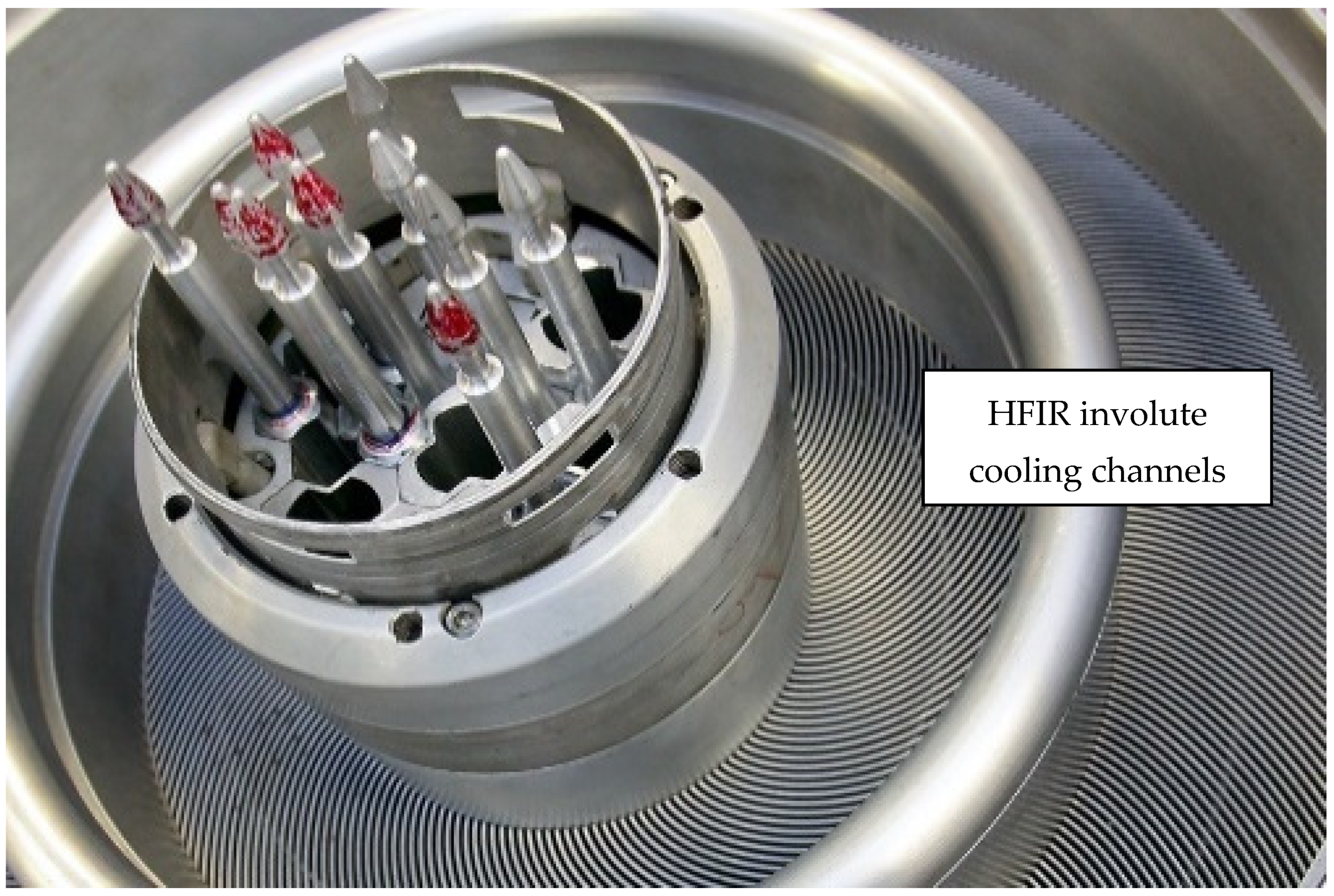
The HFIR, located at the Oak Ridge National Laboratory (ORNL), is a research and test reactor that provides very high neutron flux for a wide variety of applications. These applications range from neutron activation analysis, neutron scattering experiments, material irradiation, and isotope production. Engineering design and safety simulations are routinely used to calculate the kinematic and heat transfer properties of the coolant flow and to evaluate the reactor’s safety margins. However, such calculations must be validated to ensure accuracy. Due to the restrictive geometry of the HFIR core (Figure 1) and the high coolant mass flux necessary to maintain operating temperatures, it is impossible to instrument the flow within the core itself. And it is prohibitively expensive to construct a test loop with similar conditions. To address these issues, a flow database of high-fidelity direct numerical simulation (DNS) was developed [1]. The DNS was computationally intense, resulting in a mesh size of 10 billion elements and necessitating the use of 50 thousand central processing units to solve the discretized Navier–Stokes equations. With the database in hand, the goal at this point of the research is to develop a Reynolds-averaged Navier–Stokes (RANS) turbulence model capable of delivering the accuracy of the DNS results at a fraction of the computational expense. The study explores a novel high y+ wall function-based modeling approach and improves its prediction by modifying the loss term in the dissipation equation. Similar high-fidelity numerical simulations [2], although using different methods, were widely published before.
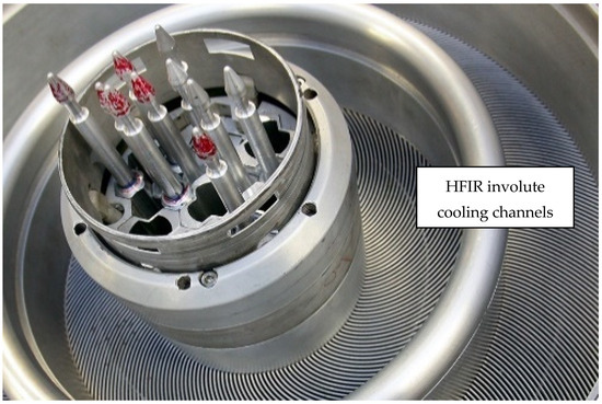
Figure 1.
The HFIR core. The fuel plates are the curved elements arranged in two rings around the central flux trap. The coolant channels are the slots that separate the fuel plates. One of these channels is modeled in this study.
2. Problem Formulation
The code selected for this application was the popular open-source software OpenFOAM [3]. It has grown a large user community over the years because it is readily available, relative to commercial codes, and because of the broad spectrum of existing applications. OpenFOAM can simulate a wide range of problem scales up to a full resolution of turbulence (DNS). For this study, a RANS model was selected that can capture the effects of turbulence on mean flow parameters without necessitating a computationally intense simulation. The k-ω shear-stress transport (SST) model was chosen because of its reputation as a popular, generally accurate model for a wide variety of applications, ranging from aerospace to nuclear thermal hydraulics [4]. The problem was approached in three stages. First, a “blind” application of the RANS model to the HFIR geometry was conducted and compared with the database results to evaluate the model performance, as implemented originally in OpenFOAM. Second, the results were assessed, the discrepancies were determined, the model was reevaluated, and modifications were applied. Third, a series of analyses were performed to generalize the introduced changes for parallel channel flows.
3. Computational Domain and Grid
A domain representing a single HFIR involute cooling channel of around 120 hydraulic diameters in length was computed, which is about half of the physical size (Figure 1). The grid was composed of hexahedral elements with curved edges to capture the involute shape of the channel. For grid generation, a simple domain decomposition was applied with the blockMesh utility provided as part of the OpenFoam package. More information about the mesh generator can be found in the OpenFOAM User Guide [3]. This grid generation method provides full control over the element distribution in any direction. The geometry was specified using a combination of straight lines and high-order splines to match the curved shape of the HFIR channel. In total, 19 interpolation points were used to define each spline, and all arc lengths were verified to ±0.01 mm of the nominal dimensions. A comparison of the DNS [1] and RANS grids is provided in Table 1. The computing load reduction is evident from this comparison.

Table 1.
DNS cyclic grid details compared with the RANS grid expressed in relative units.
3.1. Grid Node Positioning and Boundary Conditions
The grid is significantly longer in the streamwise direction, equivalent to 480δ, because it is intended for an inlet–outlet type of problem and is more representative of the real HFIR channel. The first-to-the-wall layer thickness for both the gapwise and side walls was placed outside of the viscous sublayer. This feature defines the problem as a high y+ RANS problem. Placing the first element outside of the viscous layer saves computational resources and significantly simplifies the engineering modeling of HFIR flow. Otherwise, the layer must be resolved, which imposes an additional computing burden on the simulations, making them often unaffordable in engineering types of simulations.
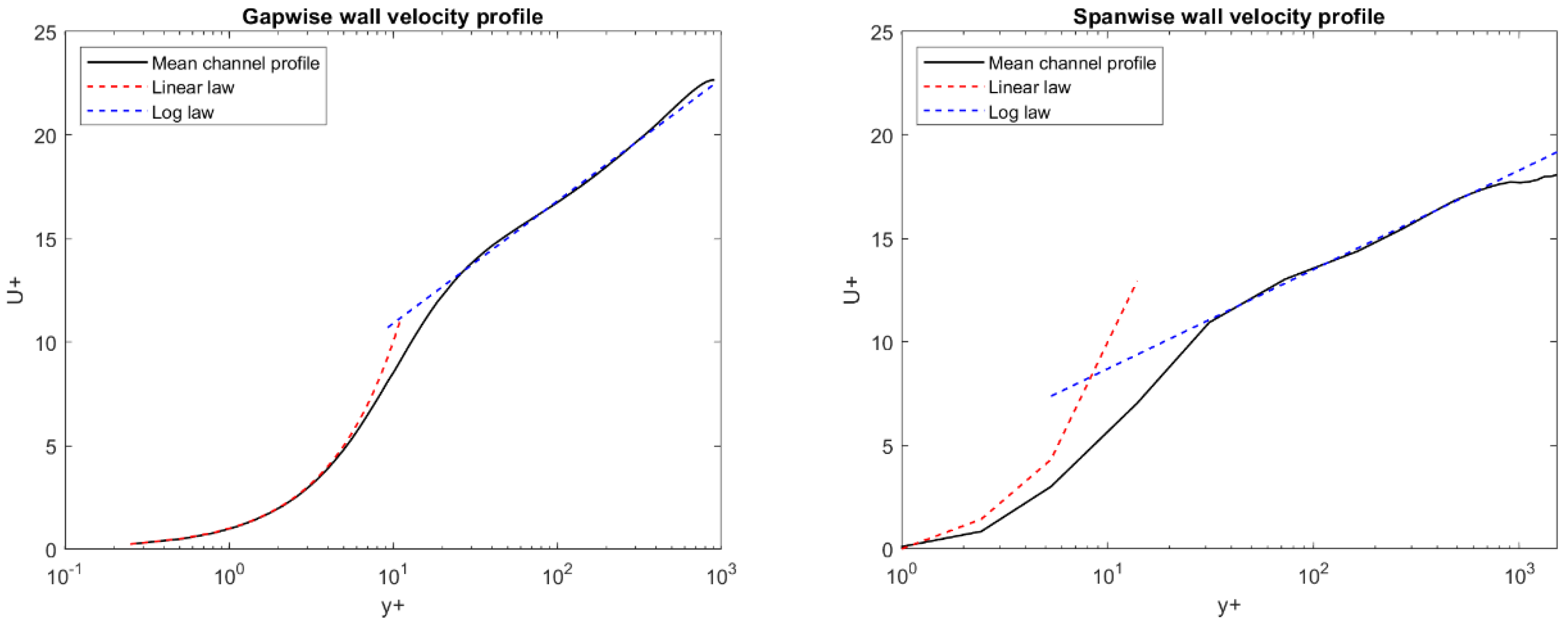
The plots shown in Figure 2, based on the DNS database [1], illustrate the principle. The plots show that the linear (red) dependency between the nondimensional velocity and distance meets the log profile at around y+ = 10. The first node of the RANS grid was placed at y+ = 20 from both walls. The mesh had 532,875 hexagonal cells distributed in streamwise, gapwise, and spanwise directions, as follows: 203 × 21 × 125. The mesh was graded to provide increased resolution near the walls, as is depicted in Figure 3. The boundary conditions applied to this problem are listed in Table 2. The inlet velocity was taken from the HFIR database [1]. The maximum aspect ratio of the grid is 177.
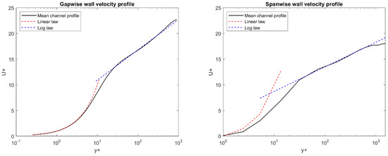
Figure 2.
DNS velocity profiles illustrating extent of viscous sublayer on gapwise wall (left) and spanwise wall (right) from [1].

Figure 3.
RANS grid., channel center (left), and channel corner (right).

Table 2.
Boundary conditions for the RANS problem.
3.2. Grid Convergence
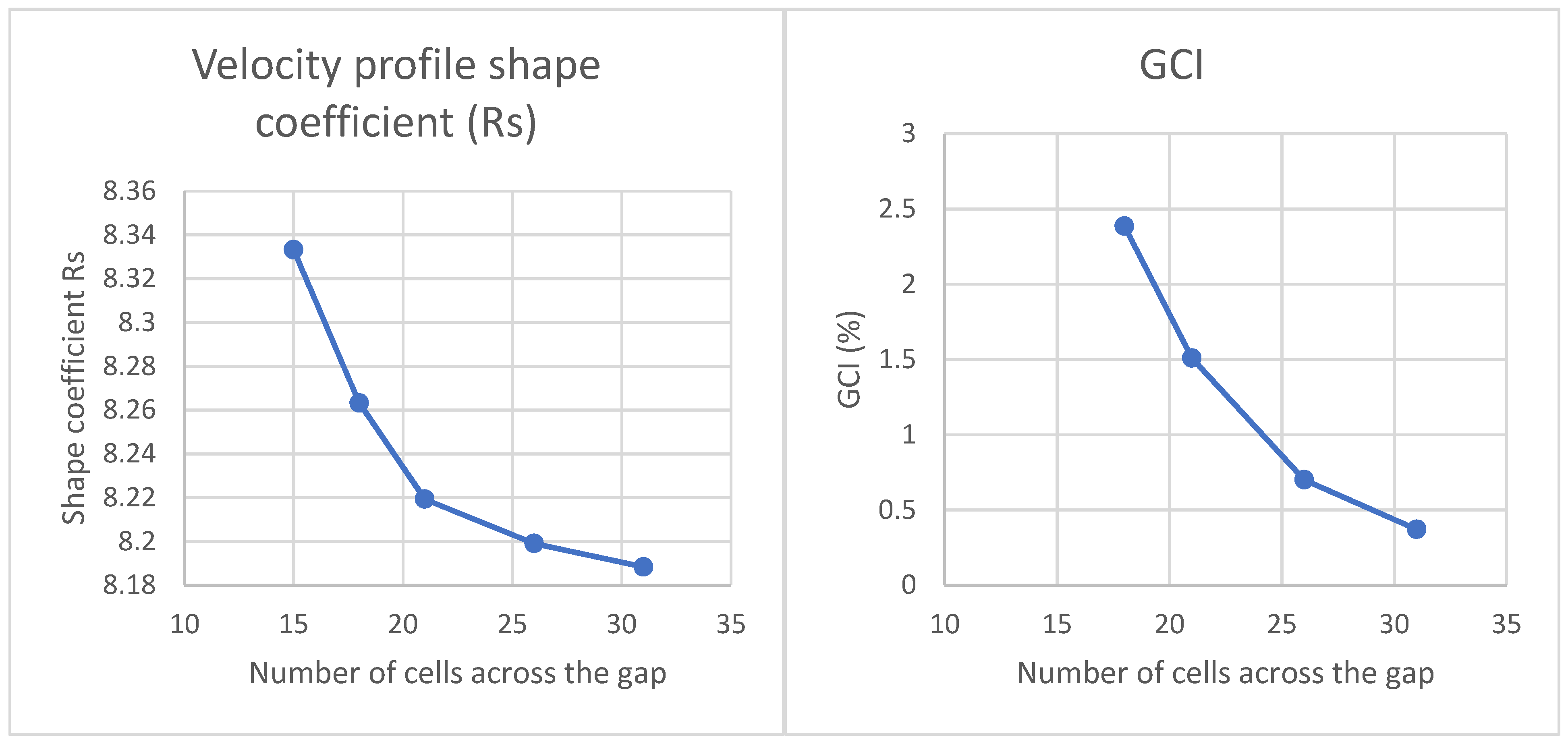
A grid convergence study was conducted to ensure that the grid resolution is properly selected and the estimated uncertainty of the spatial discretization is acceptable. The study was carried out using the grid convergence index (GCI) theory outlined in Roache [5]. As the GCI approaches 0%, the numerical result theoretically approaches the exact solution. GCI is computed by Equation (1):
where Fs is a factor and is equal to 1.25 when comparing more than three meshes, r is the uniform refinement ratio chosen to be 1.2, p is the order of accuracy of the solver equal to 2, and f is a figure of merit to be compared between meshes i and i + 1. Given the focus of the present study on turbulence modeling, the bulk velocity profile shape factor Rs from the relation in Equation (2) was selected as the figure of merit.
where UCL is the centerline velocity and the superscript + denotes wall units. The meshes selected for the convergence study are summarized in Table 3, with the computed Rs and GCI plotted in Figure 4. It is apparent that GCI converges to a very low value with increased refinement, indicating that, as the cell size approaches zero, the exact solution is obtained. Owing to the good convergence exhibited starting with the third mesh, the 532,875-cell mesh was chosen for performing the analysis. Note that the database results indicated that Rs should be 14.2, as opposed to the value of approximately 8.18 to which the RANS model converges, which is one of the initially observed discrepancies.

Table 3.
Summary of meshes used in the grid convergence study.
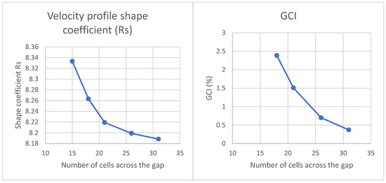
Figure 4.
Results of grid convergence study. Velocity shape factor Rs (left) and computed GCI (right).
4. Menter’s SST RANS Model
This RANS model was selected because it is one of the most popular among the engineering computational fluid dynamics (CFD) applications. The motivation for developing the k-ω SST model was to combine the advantages of the standard k-ε and k-ω models [4]. Specifically, the advantage of the k-ε is its insensitivity to free-stream dissipation values, whereas the k-ω model is much more accurate in the boundary layer by comparison with the test data. The idea behind the SST model is to switch from one model to the other outside the boundary layer. The basic approach is to multiply the k-ε equations by a blending function F1, multiply the k-ω equations by (1 − F1), and add the two together. Additional considerations regarding the formulation of this function are covered in the following sections.
4.1. Turbulent Kinetic Energy (TKE) Equations
The base k-ω SST model implementation in OpenFOAM [3] defines the k equation as shown in Equation (3):
where k is the turbulent kinetic energy (TKE), ω is the specific dissipation rate, is the modified production term, ν is the kinematic viscosity, is a constant, and is the turbulent viscosity. The implementation follows from Menter’s work [6].
Note that the F1 blending function does not make an explicit appearance in this equation since the standard k-ε and k-ω models implement similar κ equations that differ only by a constant (σk). The left side of Equation (3) represents the material derivative of turbulent kinetic energy. The right-side terms are, from left to right, turbulence production, turbulence dissipation, and turbulence viscous diffusion.
The dissipation term requires more attention. Such an implementation presumes that only a fraction of the specific dissipation rate is used to compute the dissipation of TKE. This fraction is well-known as the coefficient beta star (β* = 0.09). By assuming this, the specific dissipation rate ω formulation inherently becomes . The rationale for this conclusion is based on the work of Wilcox [7]. Such a postulate is reflected later in this study, when the results are compared with the database. The specific dissipation rate ω is reduced by a factor of β*.
The production term is implemented with a limit of ten times the dissipation term to prevent turbulence build-up in stagnation regions, as shown in Equation (4). Note that, most of the time, the limiting value is not reached.
The dissipation term is simply a product of the turbulent kinetic energy and the specific dissipation rate with a coefficient equal to β* [8].
The SST model, as implemented in OpenFOAM, employs 12 coefficients applied to the basic conservation equation and to the blending functions. They are given in Table 4 with their default values.

Table 4.
SST model coefficients and their default values.
The coefficient is computed with the F1 blending function to fully switch from the standard k-ε model to the standard k-ω model at the boundary layer because the two models use different coefficients. This implementation is shown in Equation (5). According to this formulation, the coefficient varies in the range of 0.85–1.0.
All coefficients in the k-ω SST model are blended in this manner [4]. The eddy viscosity is computed via a second blending function as shown in Equation (6), to satisfy the framework of an eddy viscosity model without overpredicting shear stress in large adverse pressure gradients [4]:
where S is the square root of S2, where S2 = 2SijSij is defined by Equation (7), and Sij is the symmetry part of the velocity gradient tensor or the strain rate tensor.
By definition, the turbulent viscosity, used as a substitute for the Reynolds stress tensor in the RANS modeling paradigm, is formulated by Equation (8). The database contains all the necessary information for the computation of the true turbulence viscosity, including the Reynolds stress components and the mean velocity derivatives.
where u’ denotes fluctuating velocity components, the overbar denotes averaging, and U capital is a mean velocity.
4.2. Blending Functions
The SST model blends both the TKE and the dissipation rate conservation equations by two blending functions, F1 and F2. They require elevated attention because the formulations depend strongly on k and ω and their distribution across the channel.
4.2.1. F1 Blending Function
The blending function F1 is defined in Equations (9) and (10) [3]:
The meaning behind the terms in Equation (10), as defined in the original paper [4], is worth discussing. The term represents the turbulence length scale divided by the distance to the wall—y. According to Menter, this term should be around 2.5 in the log layer and approach 0 toward the outer boundary layer edge. The term is supposed to maintain the value of F1 at one within the viscous sublayer. This is because it exhibits a roughly constant value near the wall and decays to zero in the log region. The term is proposed as an additional safeguard against a freestream-dependent solution. The term CDkω is defined in Equation (11).
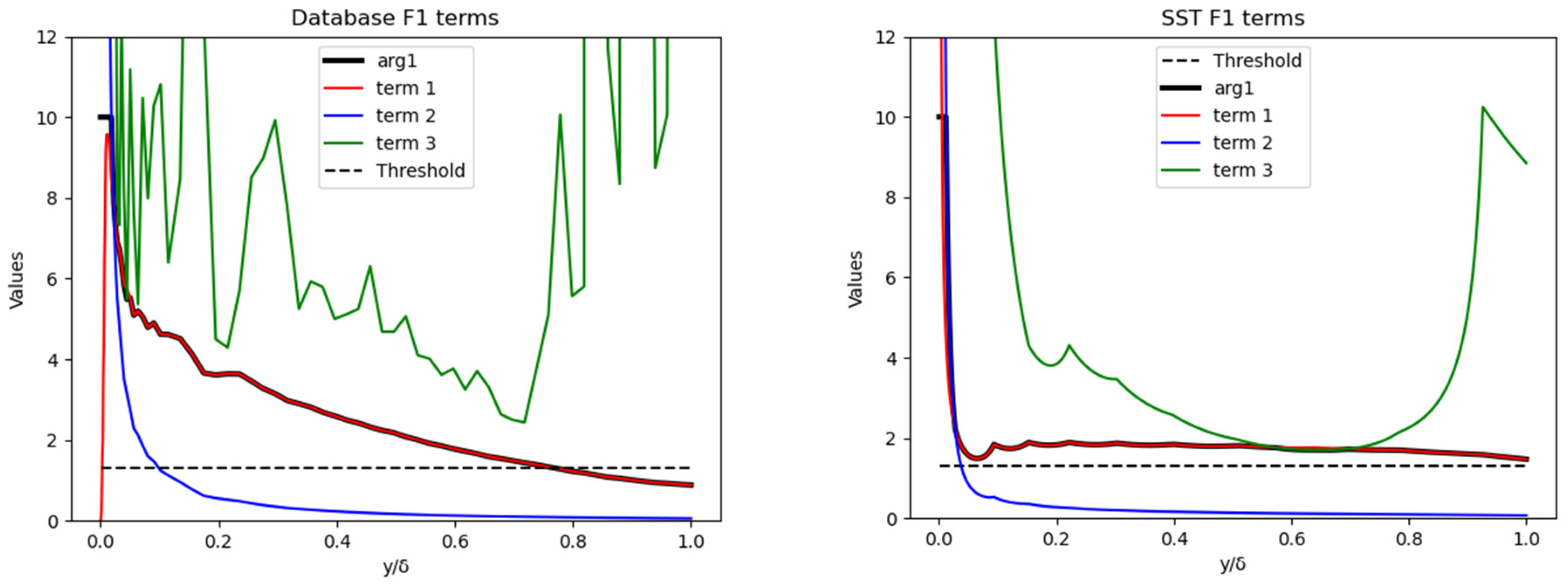
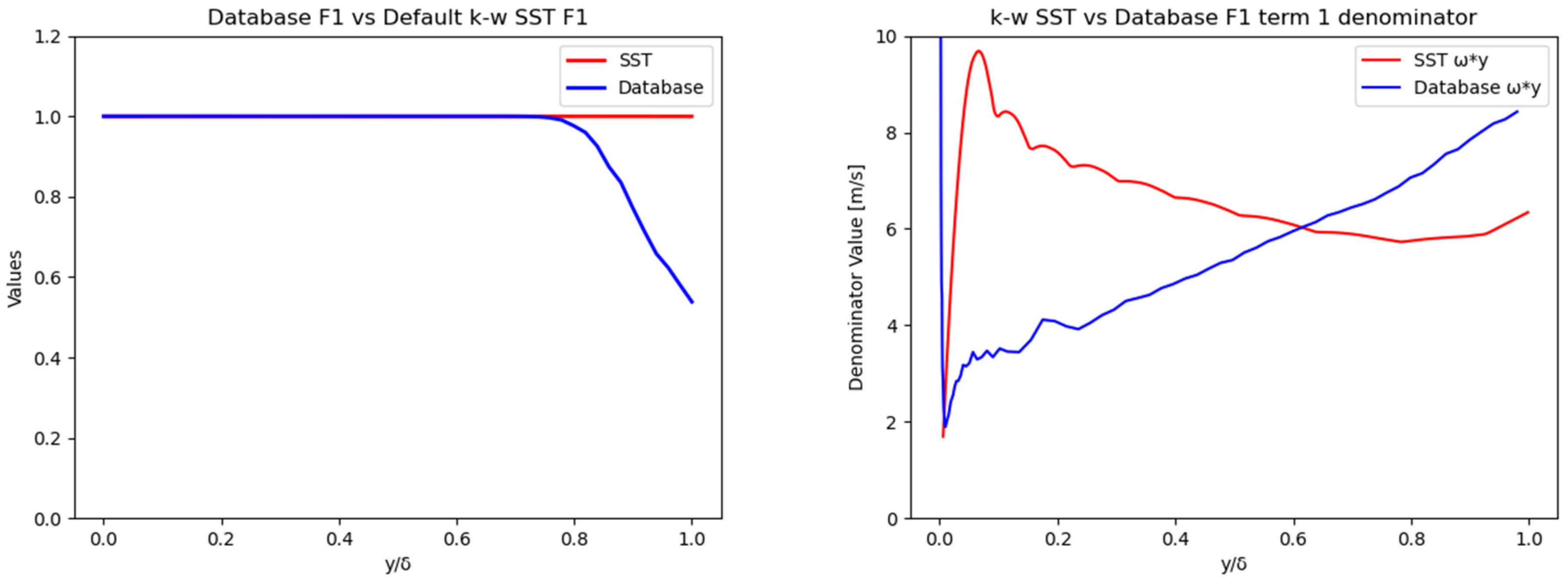
The components and the overall value of arg1 are plotted in Figure 5 for the fully developed turbulent flow in the HFIR channel (right plot) and by using data from the database (left plot). According to the SST model, the blending function F1 takes a value of 1 throughout the whole channel gap, since arg1 is above the threshold of approximately 1.3 (Figure 6, left). This implies that the boundary layer thickness for HFIR flow would be larger than the channel half-width, and therefore, only the k-ω model would be triggered. For most of the channel width, Equation (10) takes the value of the first term, except very close to the wall and in a narrow region around y/δ~0.6. The database result shows a different response. It predicts that some mixing between k-ε and k-ω should occur in the range y/δ = 0.8–1.0. This difference is mostly driven by the denominator value of term 1 in Equation (10) (Figure 6, right plot), which strongly depends on the specific dissipation.
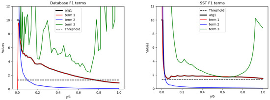
Figure 5.
F1 component distribution in the gap. The left plot shows F1 based on the database results, and the right plot shows F1 as computed in the SST model. The threshold value of arg1, at which F1 becomes noticeably less than 1, is shown as a dashed line.
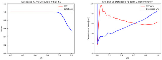
Figure 6.
F1 discrepancy between SST and database (left) and the corresponding difference in the denominator of term 1 (right).
The review of the F1 blending function revealed that mainly the k-ω model should be used for simulating the HFIR flow. The database predicted that some partial (up to 50%) mixing with the k-ε model should happen in the mid-channel. This mixing would only slightly affect the TKE conservation equation, where the factor σκ may vary only in the range of 0.85–0.92. And this factor applies only to the diffusion term of TKE.
4.2.2. F2 Blending Functions
The blending function F2 is defined in Equations (12) and (13) [3]:
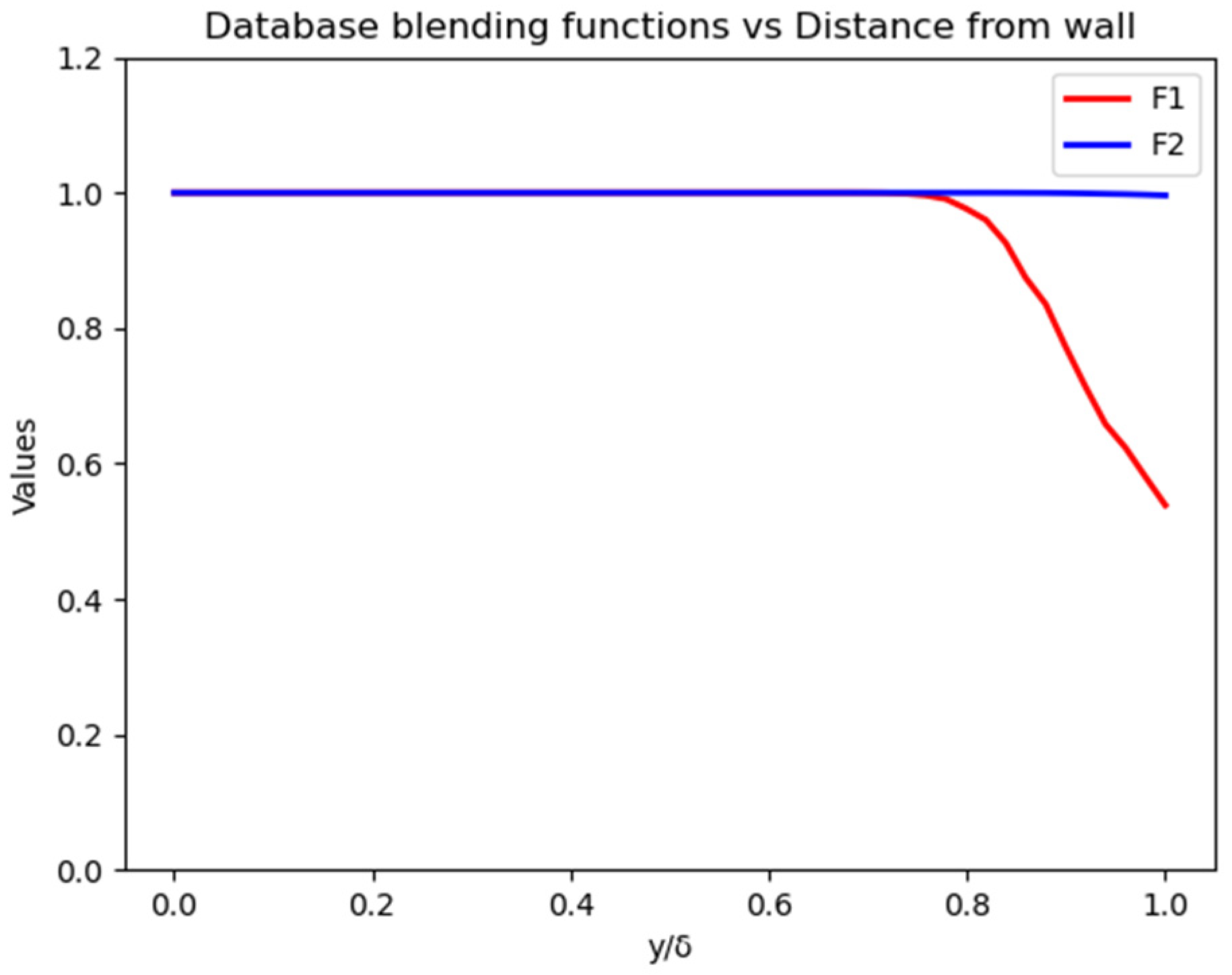
Equation (13) contains similar terms to Equation (10), except for the additional safeguard against freestream dependence, where term 1 is in fact doubled compared with the Equation (10) term 1. It comes as no surprise then that F2 takes a value of one throughout the channel in both the database and SST implementation. This function has limited use only in the expression for the turbulent viscosity given by Equation (6). Both functions are shown in Figure 7.

Figure 7.
F1 and F2 distributions from wall to channel center.
4.3. Specific Dissipation Rate Equation
The base k-ω SST model implementation in OpenFOAM [3] defines the ω equation as shown in Equation (14):
where S is defined in Equation (7), νt is defined in Equation (6), and F1 is defined in Equation (9). The blending coefficients α, β, σω, and γ are defined in Equations (16)–(19).
Equation (14) is to some extent simplified to reduce the complexity of the low-order terms. Based on evaluations by the authors, after a review of the Menter papers [4,6,8], a more comprehensive form of Equation (14) should look like Equation (15):
Two extra κ-derivative terms appear on the right side. However, Menter in [4] explicitly says that these terms are small compared with the ω terms and do not play a major role in the overall balance. Further, in this work, Equation (14) is considered comprehensive enough to allow for a transition between the k-ω and k-ε models by varying only the blending function F1, which is embedded in the free coefficients preceding each of the terms, as shown in Equations (16)–(19).
It was shown earlier that, for HFIR flow, F1 may vary in the range of 0.5–1.0 and only in the mid-channel. It is interesting to evaluate how these variations affect the SST model predictions of the main turbulence properties. This evaluation is carried out below.
5. Baseline SST Model Performance
Initial simulations were executed with the default implementation of the SST model in OpenFOAM. These simulations were intended to provide insights regarding the accuracy of the SST model when it is “blindly” applied to the HFIR problem. Such blind simulations, when the RANS models are used as developed, are commonly encountered in engineering practices.
Because the viscous sublayer was not resolved in the RANS model, the accuracy in the calculation of the first node velocity becomes increasingly important. The method for calculation of the first node velocity in the SST model was examined, and the results are presented briefly in Section 5.1.
5.1. First Node Velocity
When the first-to-the-wall node resides outside of the viscous layer, the SST model estimates the node velocity using the logarithmic law approximation. The velocity is computed as shown by Equation (20) [3].
where k is the von Karman constant equal to 0.41 and E is a roughness coefficient equal to 9.8 for smooth walls. U+ and y+ are the nondimensional velocity and wall distance computed by Equation (21).
To use Equation (21) for computing the dimensional first node velocity U1, the frictional velocity uτ must be known. In OpenFOAM, uτ is iteratively calculated. The initial guess is based on the velocity gradient:
Subsequent iteration over the following equations occurs until they converge to a specified error and iteration tolerance, as shown by Equation (23):
Once the frictional velocity is computed, the first node velocity can be calculated from the logarithmic law. The database provides results for the full velocity profile, including the viscous layer. These results were used to benchmark the first node velocity in the SST model. The velocity computed in the database was fit with a logarithmic expression, which is given by Equation (24).
Table 5 summarizes the results for the frictional and first node velocities from the SST model, the database, and Equation (24), which approximates the database result. The velocity was also computed for both (convex and concave) involute channel walls for completeness.

Table 5.
Comparison of friction velocity and first node velocity.
As seen in Table 5, the values for uτ are acceptably close, keeping in mind that this is an overall quantity. Regarding the U1 calculation, a test was implemented to evaluate the sensitivity of the entire model, including the blending functions, to the first node velocity. Equation (24) was implemented in the SST model, replacing the original Equation (22), and the result is provided in the last row of Table 5. The computed values for U1 are close. Replacing the log expression in the SST model gives little advantage, and it is not worth the programming effort. It can be concluded that the first node velocity calculation, as implemented, is accurate enough for properly simulating the HFIR velocity at that location.
5.2. Blind Model Application
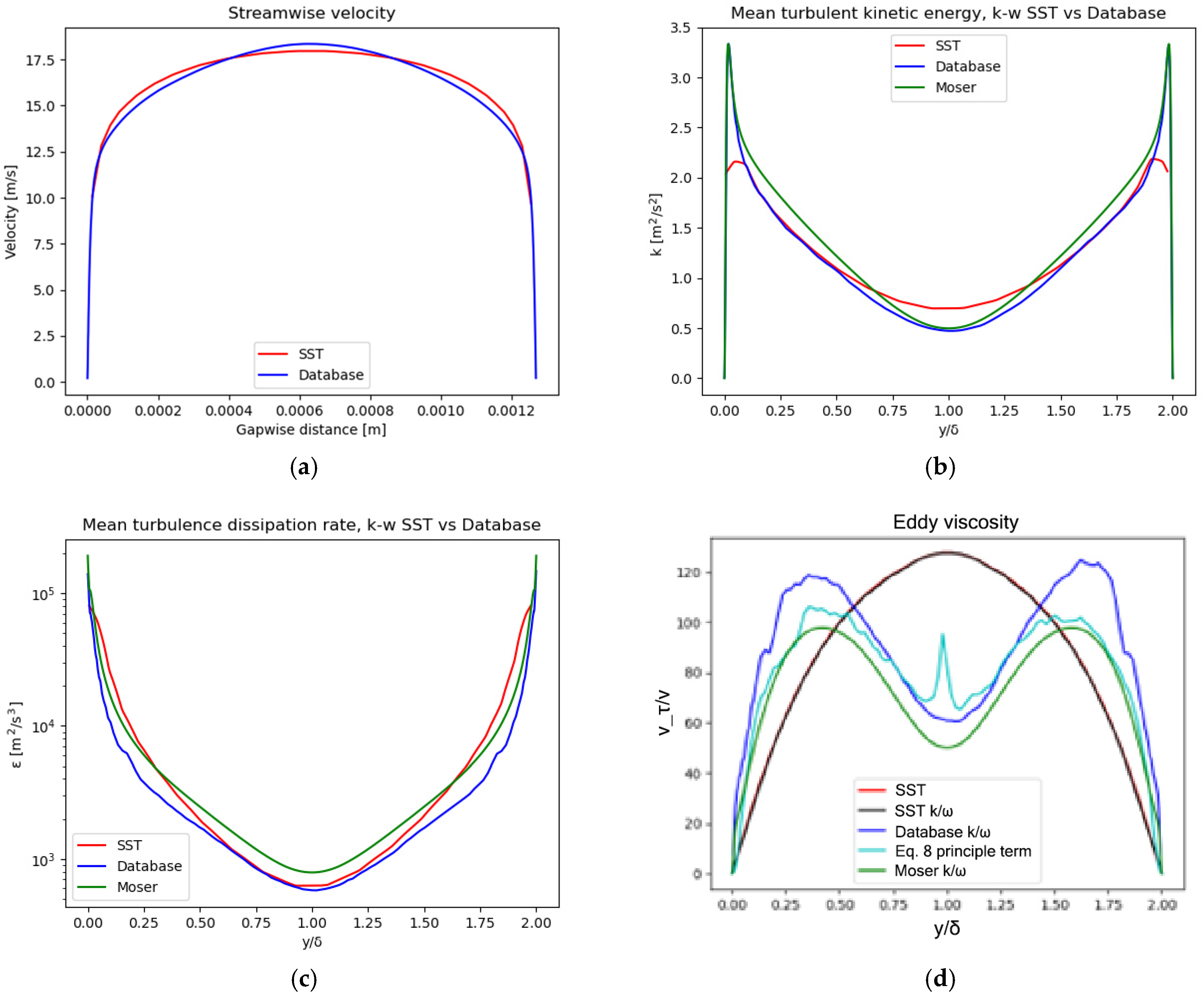
The mean velocity, turbulent viscosity, and main turbulence properties in the channel were computed with the SST model, without any model modification, and are plotted in Figure 8 alongside the database results. It is apparent that the default SST model overpredicts the TKE in the center of the channel and strongly underpredicts it next to the wall, which flattens the velocity profile. The TKE distributions were integrated over the profiles shown in Figure 8b, and the values are very close (database TKE = 0.00153 versus SST TKE = 0.00154). These numbers demonstrate that the total produced turbulence is the same, but the distribution in the channel is different. The RANS grid node spacing, in the range of the peak TKE, has at least 3–5 elements, which eliminates the possibility of smearing the TKE and confirms that it is, in fact, underpredicted by the SST model.
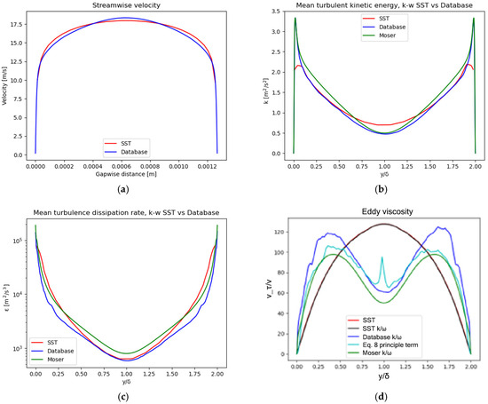
Figure 8.
Comparison of (a) mean velocity, (b) TKE, (c) dissipation, and (d) eddy viscosity profiles computed in the database, in the default SST implementation (red SST) and by simply dividing the k2 from (b) with ε from (c) (black). Data of Moser [9] are plotted in green.
A large discrepancy is observed in the dissipation rate. The plot (Figure 8c) is on a logarithmic scale and in actual units, and the result shows a significant overprediction by the SST model. This discrepancy, combined with the differences in the computation of TKE, leads to a totally different turbulent (eddy) viscosity distribution (Figure 8d). To eliminate any ambiguity, the turbulent viscosity was additionally calculated by simply dividing k by ω (or k2/ε), and the result is plotted in Figure 8d with the black line. As expected, and as shown by the plot, the two denominator formulations are almost identical and produce the same νt distribution.
The database value for νt was calculated from the database values for k and ε plotted in Figure 8b,c. However, the true formulation of the turbulent viscosity, originating in the replacement of the Reynolds stresses in the TKE conservation equation, is given by Equation (8), which is another method of calculating the turbulent viscosity. This was plotted and added to the figure in a light-blue color. The mean velocity derivative tensor and the Reynolds stresses were taken from the database. The result shows values that are lower than the database result based on κ and ε, but the profile still has two expressed humps. This result can be further explained by the slightly lower ε calculated by the database (Figure 8c).
To further verify that the discrepancy between the database and the SST model is, in fact, true, data from Moser [9] were added to Figure 8. Because these data were produced for a distinct set of conditions, they were renormalized for the conditions in the database/SST case. All compared properties deviate, but the νt profile resembles the profile computed by the database, thus confirming its validity.
It is apparent that the result is not satisfactory, and a modification is needed. Turbulent viscosity is the sole property returned from the turbulence model to the Navier–Stokes solver, and it has a major impact on the model’s accuracy. Below, the SST model implemented in OpenFOAM is analyzed to determine the most effective method for correction by using the DNS database previously generated.
5.3. SST Sensitivity to Model Factors
To improve the result, model factor sensitivity was attempted by varying only a single factor at a time. The factor values used in the sensitivity are summarized in Table 6, with their ranges based on the variation of the F1 function. These ranges were expanded by ±50% to amplify the effect.

Table 6.
Summary of coefficient values used in parametric studies.
Multiple runs were performed to evaluate the effects of the model’s factors. The results are not reported in this manuscript for the sake of brevity. This simple range-sweep type of run demonstrated that the SST model prediction cannot be qualitatively improved by varying only a single free model coefficient. In fact, the default values are often the best fit for the properties of interest. To some extent, the results can be improved by adjusting the diffusion coefficients of both TKE and ω, but such adjustments must be very substantial.
Major discrepancies are seen in the wall proximity. It is evident that the first node value in the SST for κ is much lower than in the database. The latter is true for all coefficients, including their variations. The specific dissipation rate response shows the opposite—the SST value of ω is higher at the first node. This poses the question of how these first node values for κ and ω are computed in the SST model. The bounding values of the turbulence properties are discussed in Section 6.
6. Data-Informed SST Model
Before going into the details of the conservation equations, a closer look was taken at the bounding values for κ and ω. The bounding values are the values in the first cell (face) next to the wall. In the current setup, this cell was chosen to be in the log range. This quest stemmed from the coefficients’ sweep sensitivity discussed in the previous section.
6.1. Bounding Values for Major Turbulence Properties
The SST model solves for two turbulence properties, TKE and omega. When the first cell resides in the logarithmic layer, the bounding (or the first cell value) must be computed and imposed at this cell. The OpenFoam documentation does not provide information regarding these formulations. The following discussion is based on the SST model as coded, plus open literature searches.
6.1.1. Omega Bounding Value
The bounding value for ω is set according to Equation (25). The first term is derived from a solution of an equation that applies to the viscous layer, whereas the second term is valid away from the wall. These expressions correspond to Equations (32) and (30) in the Wilcox work [7]. Equation (25) shows an option of “binomial blending”, which is the default in OpenFOAM implementation. There are other blending options; one of them is “stepwise”, in which the terms are applied separately as a function of y+. The blending concept is still to be investigated. But, because it has little justification, further in this analysis, the stepwise option was chosen. With this assumption, only the second term in Equation (25) applies, and its derivation is discussed below.
where the coefficients’ default values are in Table 4, and kappa is the von Karman constant kappa = 0.41
Following Wilcox [7], this term results from the solution of the system of equations formulated according to Equation (26).
This system is formulated for a layer of the flow “far enough from the wall to render the molecular viscosity negligible relative to eddy viscosity, yet close enough for convective effects to be negligible relative to the rate at which the turbulence is being created and destroyed”, as stated in the Wilcox paper. When the velocity is substituted with the log law expression, , and the corresponding derivatives are taken, the resulting solution yields expressions for k and ω:
Replacing the frictional velocity in those expressions produces the second term in Equation (25). It must be noted that the expression for k serves only to compute the frictional velocity in the SST model according to Equation (29). The database-computed bounding value of ω is about two-times lower, suggesting some of the coefficients in Equation (27) are not fully applicable to the HFIR channel flow.
6.1.2. TKE Bounding Value
The SST model provides two options to set the κ bounding value (k1) for the high and low y+ given by Equation (28). The high y+ option is further used in these analyses.
Equation (28) has two components in the brackets. The first one is a function of the cell distance to the wall, which is used to decrease a constant of 8.366. The second is the frictional velocity squared, as computed in the SST model and shown in Equation (29).
Equation (28) is derived through a fit to the so-called “-” model. A detailed explanation can be found in the work by Kalitzen [10]. In that work, the authors solve for the dimensionless and do not explicitly define . The implementation must use the result obtained by Wilcox in Equation (27). Because the frictional velocity is defined by the TKE, the expression becomes implicit. This, together with the overall solution for TKE, which is by default iterative, allows little flexibility for using this expression to modify the TKE bounding value. Instead, the focus was placed on the TKE production term bounding value G1, which is discussed in Section 6.1.3.
6.1.3. TKE Production Bounding Value
The production terms are the first terms on the equation’s right side. The TKE production is given by Equation (4). It has a hard limiter of ten times the dissipation rate. The production is defined after averaging the Navier–Stokes equations as the product of the tensor (G) and the turbulent viscosity. The G formulation is given by Equation (30).
The bounding value of G1 is computed by Equation (31). In the viscous layer, it is zero.
The expression for the log layer can be evaluated if the frictional velocity is known. The first two terms translate to the shear stress at the wall, which can be approximated with . And the last term in the numerator is again the frictional velocity given by Equation (28). Substituting in Equation (31) enables rewriting the G1 bounding expression as
Accounting for the first node positioning, the estimate for G1 is around twice as high as the resulting value from Equation (31).
In the preceding section, the bounding value of ω was determined to be too large in the default SST model. If this value is reduced by a constant multiplicative factor of about 0.4, the SST model generates a better prediction of the dissipation near the wall. However, this reduction of near-wall dissipation generates a larger TKE at the wall. It was found that this result could be corrected by simply reducing the value of by the same amount, about 0.4. This result suggests that, to properly compute the k and ω bounding values, another factor can be applied to the computation of frictional velocity.
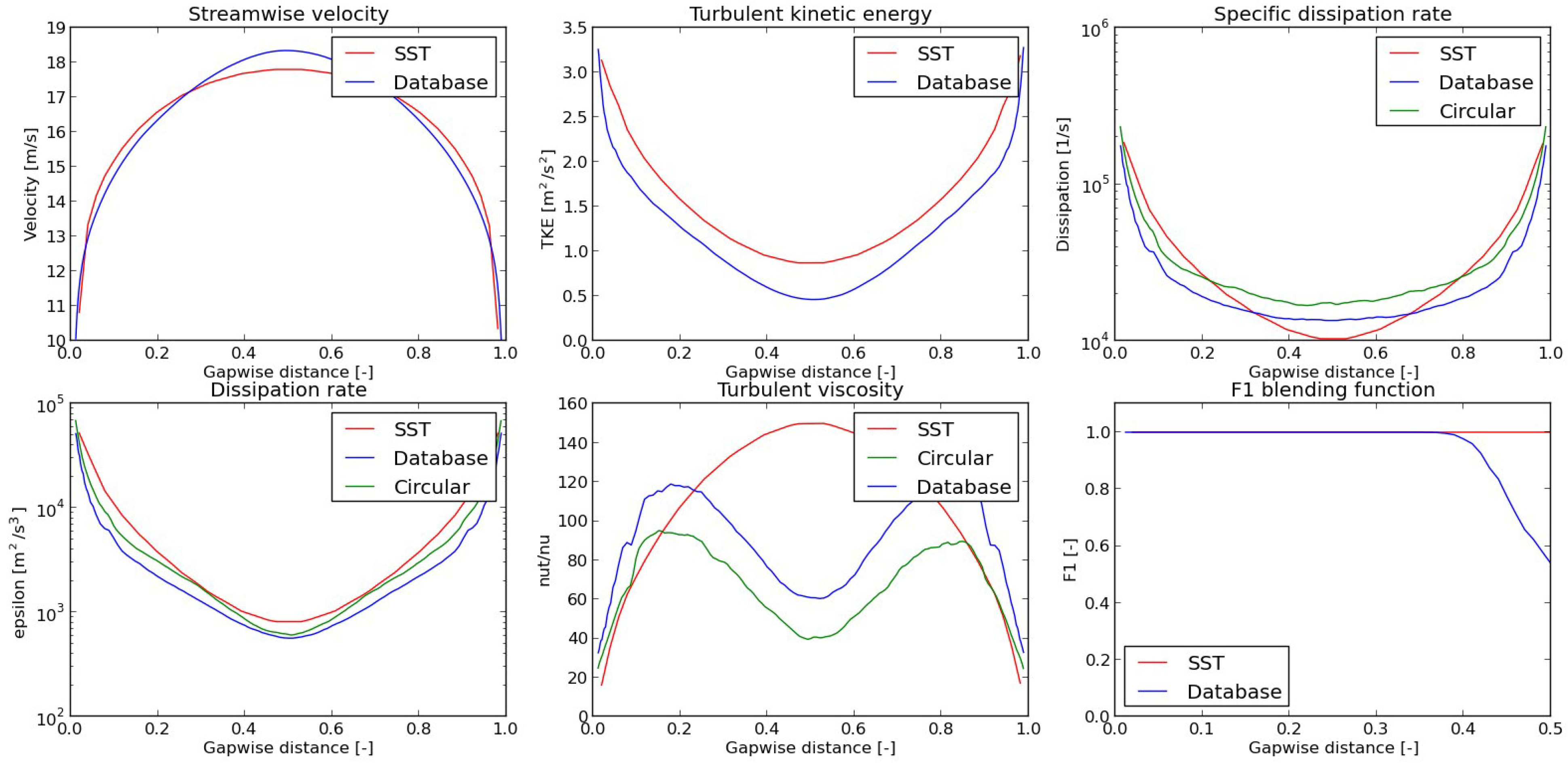
The major turbulence properties were computed and compared with the database after the bounding values for ω and G1 were corrected according to the above derivations. They are depicted in Figure 9. The model is still clearly deficient at predicting the correct profiles for nearly all quantities. The work in this section and the sensitivity study in Section 5.3 demonstrate that better accuracy cannot be obtained by just modifying the model constants and bounding values. This finding suggests that the form of the model equations is inconsistent or at least is not fully capturing the physics involved.
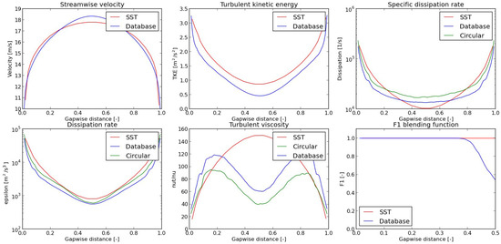
Figure 9.
Major turbulence properties after the bounding values for k and ω have been corrected to match the database.
6.2. Specific Dissipation Rate (ω) Production and Loss
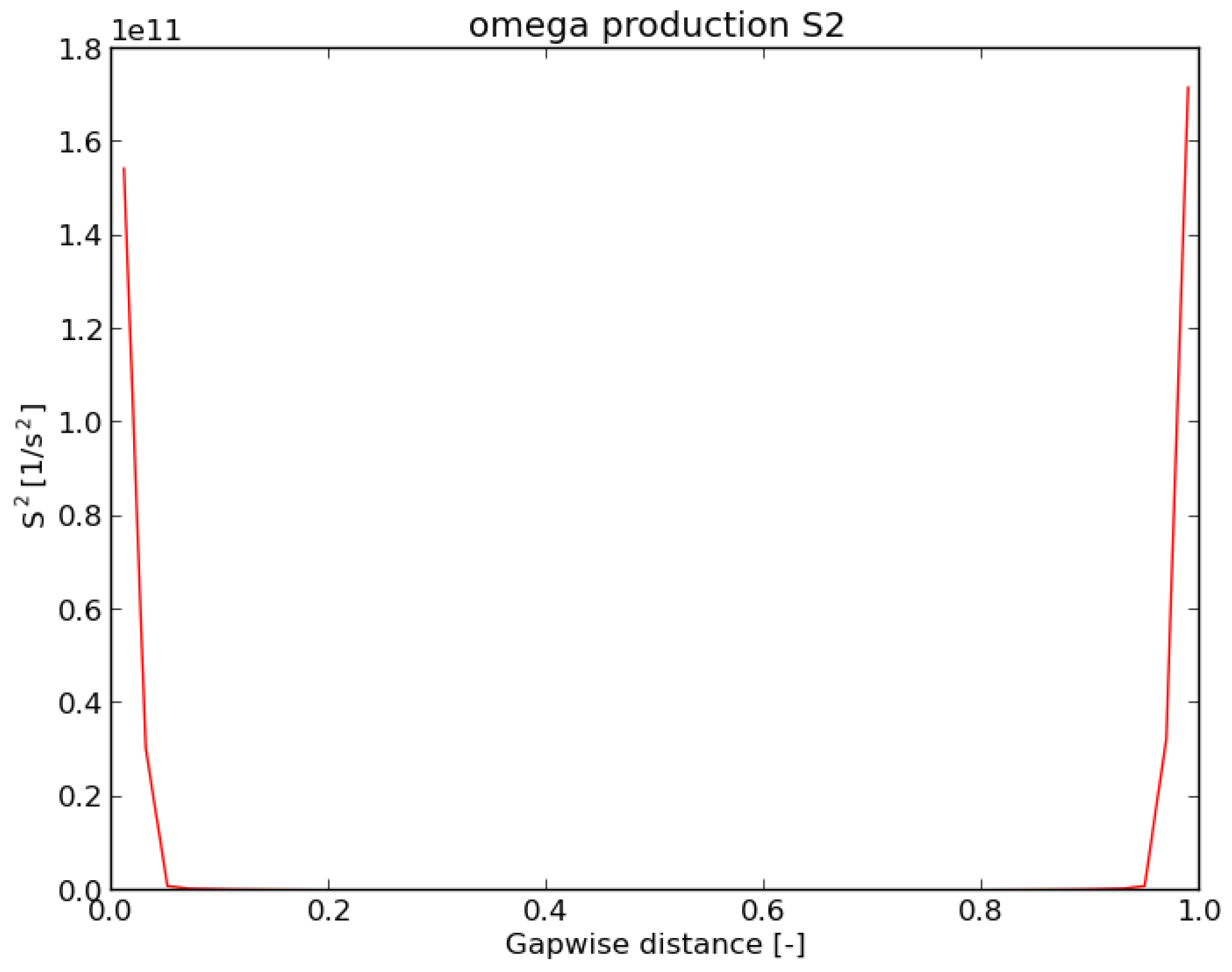
The production of ω is given by Equation (7) and represents the trace of the mean strain rate squared. The production of dissipation is expected to occur in the wall’s proximity, where the maximum shear is taking place. This is well-confirmed by plotting S2 in Figure 10. Practically no dissipation is produced in the bulk of the flow. Such a formulation of the production term was deemed credible and likely is not the cause of improper ω prediction by the model.
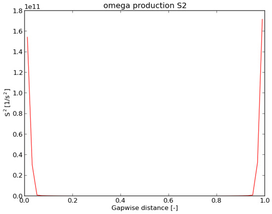
Figure 10.
Omega production distribution in channel.
The loss term is formulated in Equation (14) as omega squared. To understand this loss term formulation, one must go back to the exact dissipation equation and the reasoning used in the original k-ε model. The well-known form of the k-ε dissipation equation originates in the thesis by Hanjalic [11]. By subtracting the RANS momentum equation from the instantaneous Navier–Stokes equation, differentiating with respect to , multiplying by , and then, time averaging, an exact equation for the dissipation
can be derived (Equation (33)):
where and refer to the fluctuating velocity and pressure, and refers to the mean velocity.
Each of these terms on the right side represent forms of either production or destruction of dissipation and are explained in Hanjalic’s thesis. The terms on the right side do not have a closed form, and so, the dissipation equation cannot be solved directly. Multiple assumptions are made to simplify Equation (33) into the form found in the well-known k-ε model (Equation (34)).
Of interest is the term corresponding to the destruction of dissipation due to viscosity, as shown in Equation (35). Hanjalic [11] simply states that this term “may plausibly be expressed in approximate form as”
The original k-ω model is not significantly different from the k-ε model. The difference is that Wilcox simply solves for the specific dissipation instead of the true dissipation. By defining the specific dissipation as and noting that the k-ω model can be derived directly from the standard k-ε model [12]. However, after this variable transformation is performed, there are additional terms that are proportional to the gradient of (as in Equation (15)). If these terms are ignored, one arrives at the original k-ω model by Wilcox. When Wilcox changes variables from , the following transformation occurs to the loss term:
Changing the variables from changes each term’s dimensions to 1/s2. The form of the ω equation really is heavily dependent upon the form of the ε equation and the assumptions that go into modeling each term. It is likely that the loss term was posited based purely on a dimensional analysis. This is explicitly stated in the book by Rebollo and Lewandowski [13]. The authors state that this loss term could be the source of a totally new closure equation but that “a large number of numerical experiments conducted since the work by Launder and Spalding suggest that two closure equations are more than enough, and an additional equation do not bring greater accuracy. This is why we may close [the loss term] using dimensional analysis”.
After variables are changed from ε to ω. The ω2 form of the loss, present in the k-ω and SST models, appears. By reviewing the original literature, one can conclude that the form of the ω loss is derived based solely on a dimensional analysis. This conclusion cannot really be trusted on physical grounds, since it involves no derivation from fundamental theories. Its only justification is that it balances the units of other terms in the equation ( in the case of the ω equation, and in the ε equation). The k-ω and k-ε turbulence models are widely used because of their empirically observed value. If the interest is only in the empirical results, then new expressions for the loss can be suggested, which are not necessarily physical as long as they generate accurate results.
The real implementation of the loss term is implicit and means that ω is decreased by a factor equal to itself, i.e., to ω, which produces the square. This is the major factor leading to the parabolic shape of ω seen in Figure 9. It is evident that the loss is excessive in the mid-channel and insufficient next to the wall when applied to HFIR. Suggesting another dependency for the loss as a linear function of ω and S produces the desired results. The general form of that function is given by Equation (37).
The best result for application to the HFIR was achieved with a = 1 × 10⁻⁵, b = c = 2. In order for this new form to have correct units, the constant a must have units of . This formulation improves the result primarily because of S2 term inclusion. A plausible physical explanation could be because the dissipation is generated and destroyed in the same vicinity of the wall proximity.
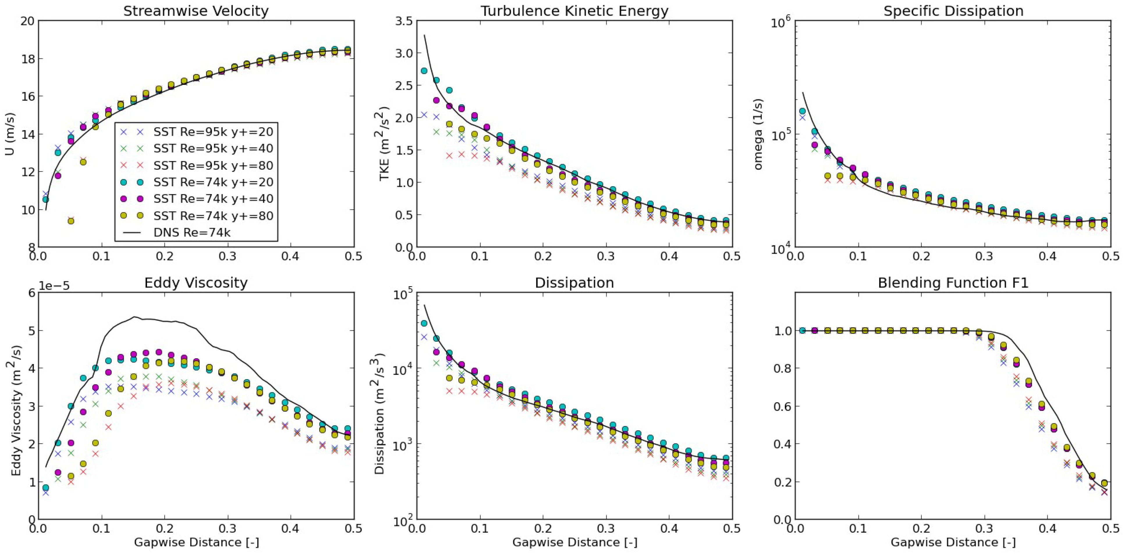
After the implementation of these modifications to the SST model, runs were performed for the estimated limiting HFIR Reynolds (Re) numbers of a minimum of 74,000 and a maximum of 95,000. The database flow conditions were chosen for the minimum Reynolds flow number. Both runs are plotted in Figure 11, with circles for the low Re and crosses for the high Re number. The Re number mostly affects the TKE and the viscosity distributions. In general, the lower Re number run better matches with the database, which is an indication of relevance.
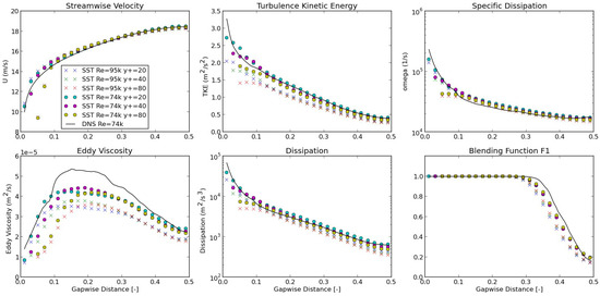
Figure 11.
Modified SST model results for a range of HFIR-specific Reynolds numbers and meshes with different y+. The SST model implementation includes the modified sink term, with and decreased by the same factor.
The effect of the mesh was also tested by running the new SST implementation with different meshes, each with a different for the first node off the wall. Table 7 describes the mesh parameters. The higher meshes use the same total number of cells and the same number of cells across the gap (21), with uniform spacing (no grading). This arrangement results in slightly higher bulk resolution. These results are also shown in Figure 11. The meshes with deviate from the database in the wall proximity but show fair agreement toward the center of the channel. The best results occur for the meshes with a . A lower might also improve performance because the k-ω model is valid within the viscous sublayer, but determining whether that is so was not an objective because it would incur extra computational cost.

Table 7.
Mesh specifications for new SST model tests.
Based on this assessment, it can be concluded that the new SST implementation properly simulates the turbulence of HFIR flow in the entire range of Re numbers with moderate-to-low computational resources and can be used for engineering modeling purposes.
6.3. SST Model Generalization for Channel Flows
In the sections above, changes to the SST model were proposed after analyzing the derivations for certain wall functions and the loss term in the specific dissipation equation. Specifically, it was observed that the default bounding value for TKE production () was low and the bounding value for specific dissipation () was high when the HFIR channel flow was simulated. These values were corrected by reducing each bounding value by the same constant. In the specific dissipation equation, the loss term was modified according to Equation (37). All these changes together produced a model that better captured HFIR profiles of the streamwise velocity and other turbulence quantities.
These modifications were made based on the database simulation at a single HFIR Reynolds number. Therefore, the introduced changes were specific to the dataset used. To further extend the model to general channel flows, more conditions were analyzed at different Reynolds numbers.
The next section reviews an additional study that was carried out to help generalize the model. The model was evaluated on a simple parallel channel geometry and compared against the DNS results reported by Lee and Moser [9] (referred to as “LM” hereinafter). From these tests, additional relationships were derived that helped generalize the model to a wider range of conditions.
A series of tests was performed using a simple parallel channel geometry (Figure 12). The geometry is identical to that of the LM, with a streamwise length of about , a spanwise length of , and a wall-to-wall distance of 2δ.
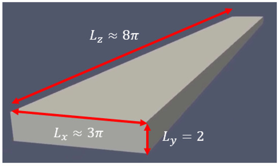
Figure 12.
Parallel-plate geometry for channel flow testing. Units are in half-gap width—δ.
Periodic boundary conditions were applied in the spanwise (x) and streamwise (z) directions. The OpenFOAM mean velocity force option was used to keep the average streamwise velocity constant. This was accomplished by dynamically adjusting the pressure gradient, which was the same method used by the LM. Also following the LM, only the kinematic viscosity was varied to reproduce the corresponding frictional Reynolds (Reτ) number. In the following, the “baseline SST” refers to the original Menter’s formulation, and the “new SST” refers to the modified implementation. For each Reynolds number, the mesh was adjusted to keep the in the range of 20–30.
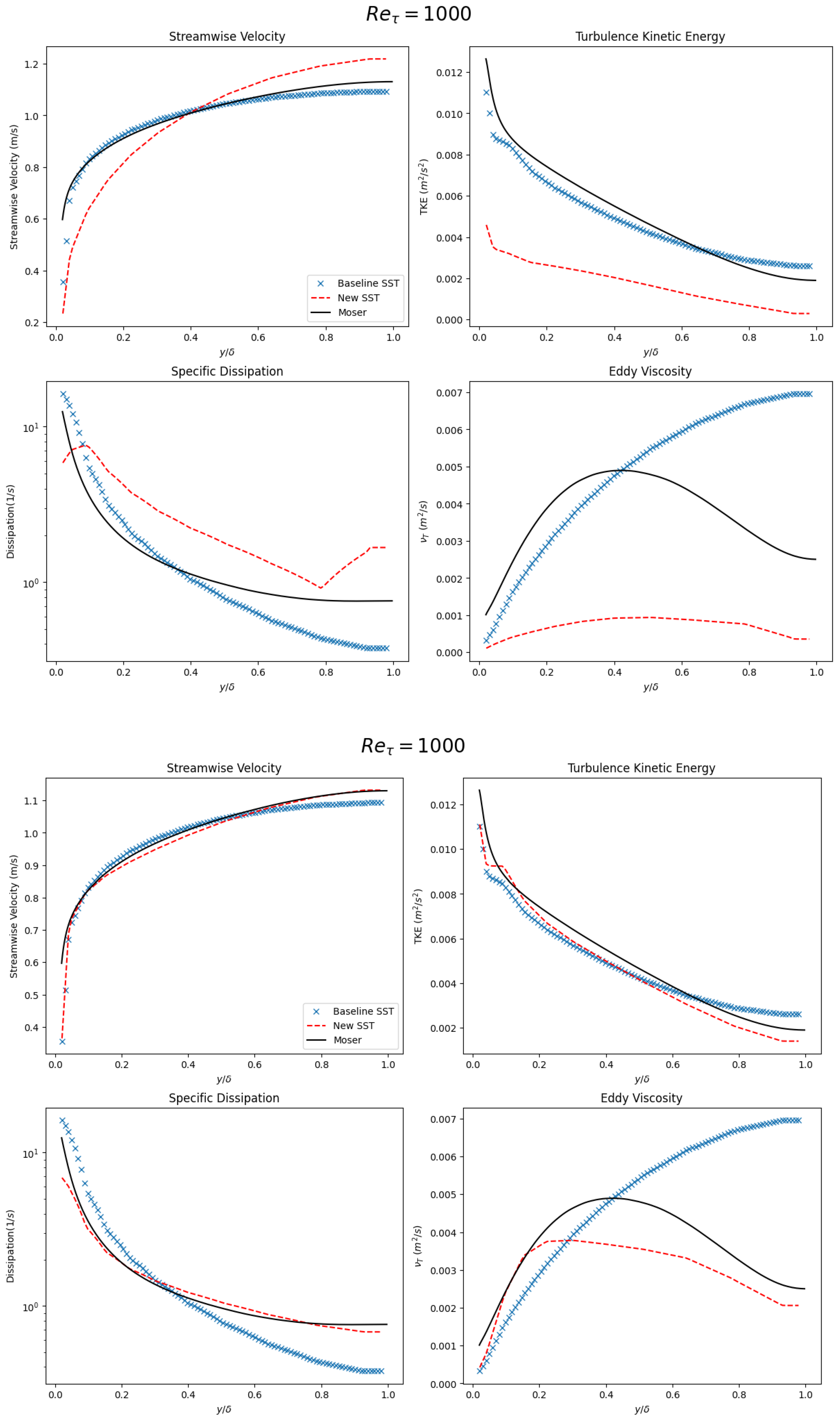
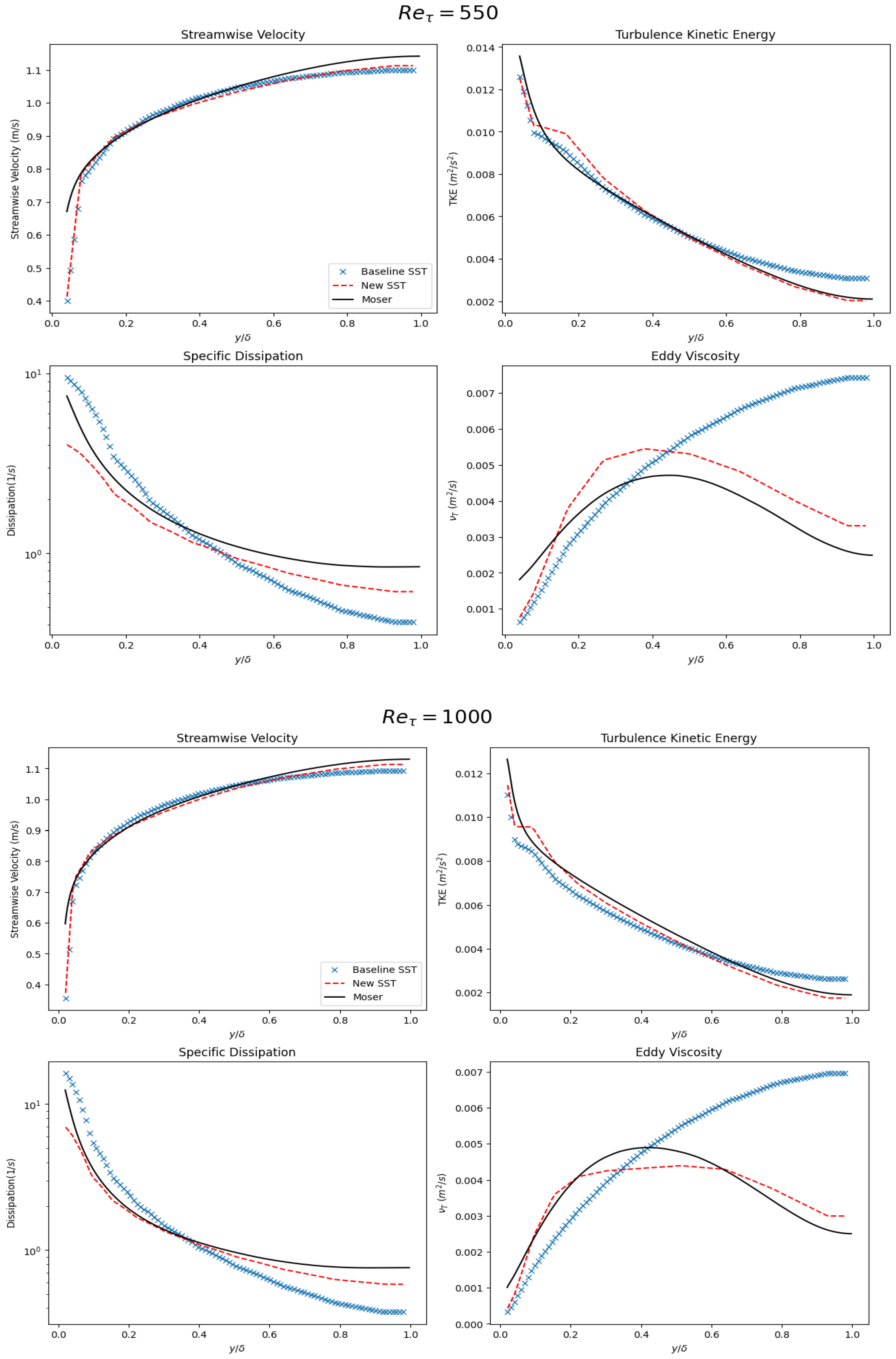
The new model, with the modified loss term given by Equation (37) and the new bounding values for ω and was first tested on the case, which is the closest to the HFIR of 960. This result is shown in the top four plots of Figure 13. Clearly, one or both constants are somehow not dependent on just .
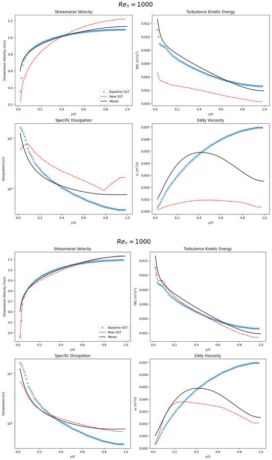
Figure 13.
Application of new model to the LM case of . Top four plots are before and bottom four are after the constant modification.
Attention was given to the constants used in Equation (37). Constant should have units of time in order to balance with the rest of the dissipation equation. An option for providing dimension to constant is to divide by the shear rate at the wall: . For the HFIR case, it was found that an of about 1 × 10⁻⁵ gave the right distribution for omega. The constant 9.37 × 10⁻⁶ s 1 × 10⁻⁵ s gives the right magnitude and units for this term. For the LM case, this constant is equal to about 0.24 s, because of the viscosity difference. This value is vastly different from that of the HFIR case, even though both cases have nearly the same frictional Reynolds number. Application of this new constant formulation produces the desired result, as shown in the bottom four plots of Figure 13.
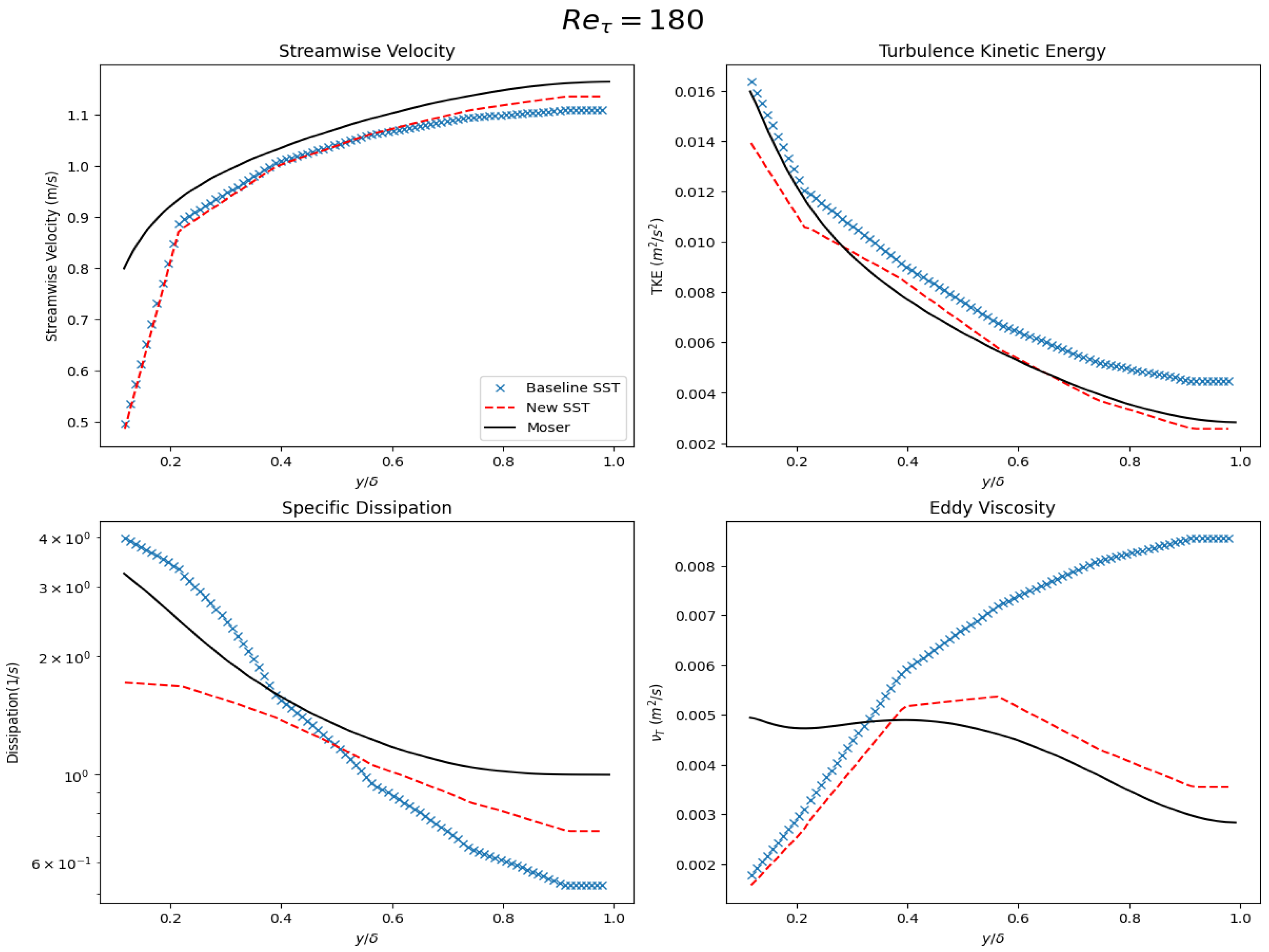
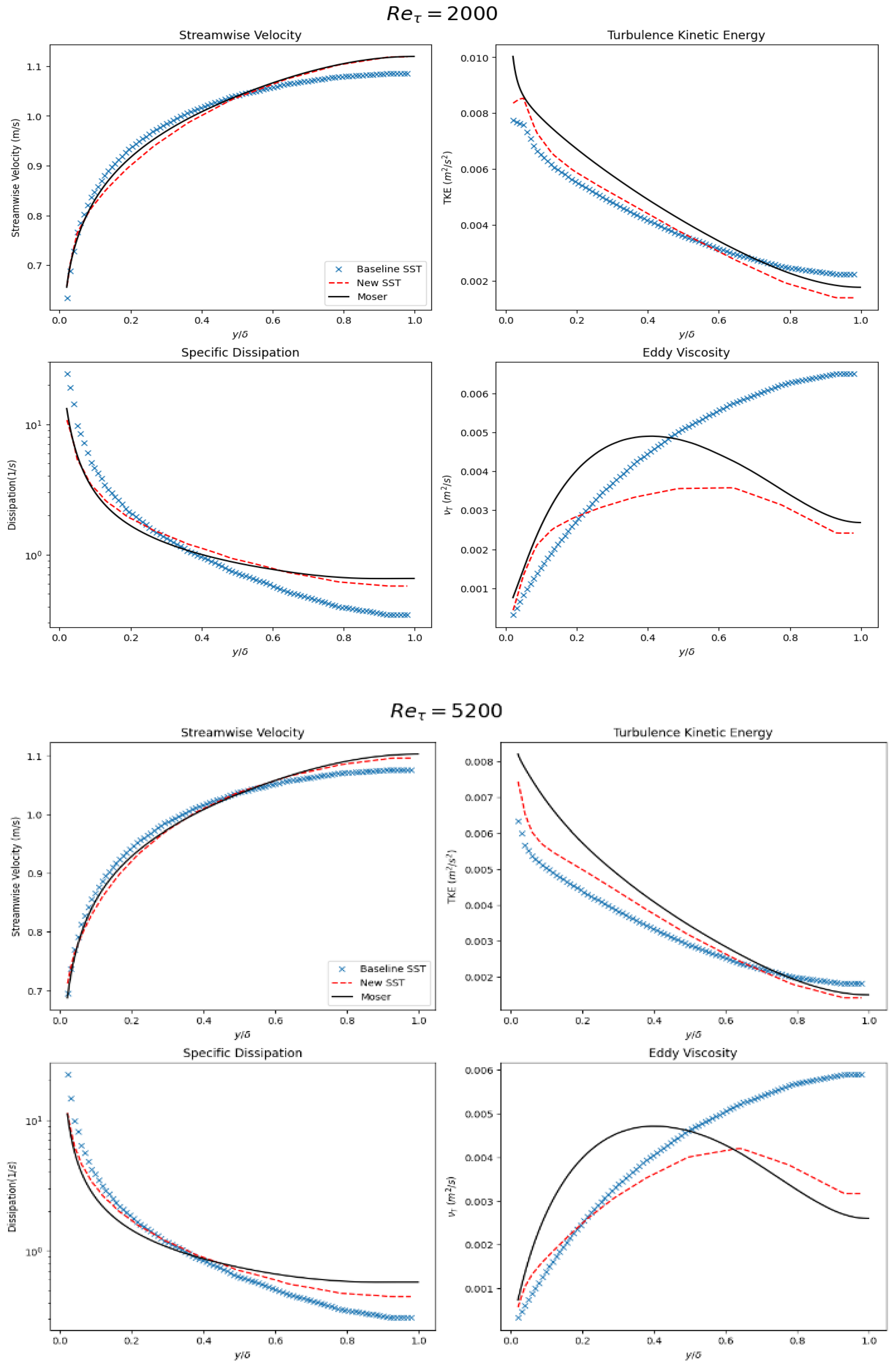
This final implementation was then tested for each of the cases reported by the LM, and the results are shown in Figure 14. The constants used are shown in Table 8. The values of viscosity and friction velocity are the exact values reported by LM. For each run, the amount of the contribution (constant c in Equation (37)) was modified slightly to provide a better fit to the DNS results, but this modification has not been heavily fine-tuned. This contribution increases slightly with , but constant changes more dramatically between the cases. In general, the new model obtains a closer fit to the DNS results. Both the original and the new SST models perform worst for the lower cases. It is interesting to note that the new model improves with higher Reynolds number flows.
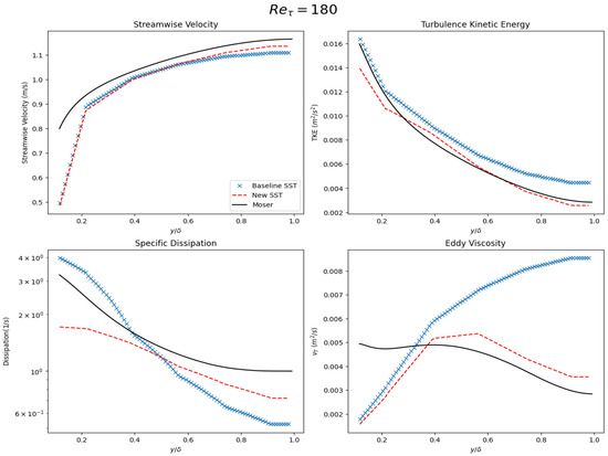
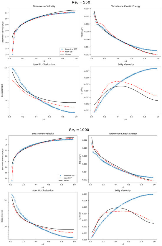
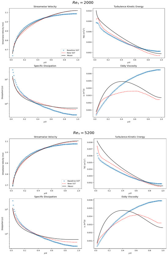
Figure 14.
Results of parallel channel tests. The new SST model is shown by the red dashed line. The original OpenFOAM SST model is shown by the blue crosses, and Moser data are shown by the black solid line.

Table 8.
Constants used in new SST model on each Lee and Moser case and HFIR.
One specific of the model is the need for the frictional velocity to be known beforehand. For many flow configurations, it can be easily estimated using the simple wall shear-stress correlation
where is the Darcy–Weisbach friction factor calculated via the Colebrook–White equation and U is the average streamwise velocity. This calculation gives a friction velocity estimate of simply , which provides a result close to the true friction velocity reported by LM. Using this estimate of instead of the true values results in a negligible change in the new SST model’s performance, and it is not reported here. In the future, the new implementation of the SST model derived here should be assessed against more data for channel flows (including experimental) to confirm its validity. It can be tried equally, as well on other channel geometries, to evaluate performance.
7. Conclusions
This work brings information obtained by high-resolution studies of HFIR flow turbulence to practical use for simplified, but still sufficiently accurate, engineering simulations. A well-known RANS model of turbulence was studied and modified to allow for the implementation of fast, computationally efficient algorithms in any CFD computer code. To achieve high performance, relatively coarse meshing was used, but relevance was demonstrated on meshes with varying y+ between 20 and 80. The runs were performed on a few (4–8) compute cores with meshes of around 0.5 M elements, and each run takes less than 5 min to execute. It was found that introducing changes in the calculation of the properties’ bounding values, and in the dissipation conservation loss term, fundamentally improved the model prediction for channel flows. The accomplishments in this work can be further developed and fine-tuned for specific applications, beyond HFIR. The focus was on the major factors leading to qualitative discrepancies. Those were identified, and methods for correction were offered. The results can be used to compute industrial channel flow turbulence in general, reactor thermal hydraulics, and other relevant applications. Additional validation work might be required to complement that performed in this study.
This study lays a foundation for research on channel flow heat transfer. Proper prediction of turbulence is the key to accurate simulation of the complex thermal phenomena occurring in the narrow HFIR channels, including heat transfer coefficients and channel pressure losses, which are critical for safe reactor operation. The research results have improved the understanding of the flow characteristics and built a foundation to improve reactor performance in the process of transitioning to low-enriched fuels.
Author Contributions
Conceptualization, E.P.; methodology, all; software, N.M. and T.G.; validation, all; writing—original draft preparation, E.P.; writing—review and editing, E.P.; visualization, T.G. and N.M. All authors have read and agreed to the published version of the manuscript.
Funding
This research was funded by Office of Material Management and Minimization (M3) of the US Department of Energy’s National Nuclear Security Administration, grant number DE-AC05-00OR22725.
Data Availability Statement
The data presented in this study are available on request from the ORNL-RRD (Research Reactor Division).
Acknowledgments
The authors would like to acknowledge the support for this work provided by the Office of Material Management and Minimization (M3) of the US Department of Energy’s National Nuclear Security Administration.
Conflicts of Interest
The authors declare no conflict of interest.
Abbreviations
| CFD | computational fluid dynamics |
| DNS | direct numerical simulation(s) |
| GCI | grid convergence index |
| HFIR | high-flux isotope reactor |
| ORNL | Oak Ridge National Laboratory |
| RANS | Reynolds-averaged Navier–Stokes |
| SST | Shear-stress transport (model) |
| TKE | turbulent kinetic energy |
| δ | half gap size used as characteristic length |
| x | streamwise direction |
| y | wall direction |
| z | spanwise direction |
| y+ | nondimensional wall distance (y+ = y uτ/ν) |
| Lx/δ, Lz/δ | domain size in gap units |
| L+x, L+z | domain size in wall units |
| ∆x+, ∆z+ | grid size in wall units |
| ∆yw+, ∆yc+ | normal-to-wall grid size, wall units, at the wall w and in the bulk c |
| Ny | resolution in y direction |
| u, v, w | instantaneous velocity components in the lab (orthogonal) coordinate system |
| U, V, W | mean values of velocity components |
| u′, v′, w′ | fluctuating components of velocity |
| ∂ui/xi | velocity derivatives tensor |
| ∂u′i/xi | fluctuating velocity derivatives tensor |
| uτ | frictional velocity |
| Re | flow Reynolds number |
| Reτ | frictional Reynolds number |
| k | turbulent kinetic energy |
| νt | eddy viscosity |
| ω | specific dissipation rate |
| p | pressure |
| ν | kinematic viscosity |
References
- Popov, E.; Bolotnov, I.; Mecham, N. Numerical Database of HFIR Flow Turbulence, ORNL TM2022/2814; Oak Ridge National Laboratory: Oak Ridge, TN, USA, 2022. [Google Scholar]
- Raisee, M.; Vahedi, N.; Rostamzadeh, A. Prediction of Gas Flow Through Short and Long 2-D Micro and Nano-Channels Using a Generalized Slip Model. In Proceedings of the ASME 2008 6th International Conference on Nanochannels, Microchannels, and Minichannels, Darmstadt, Germany, 23–25 June 2008. [Google Scholar]
- OpenCFD Ltd. OpenFOAM: User Guide. 2019. Available online: https://www.openfoam.com/ (accessed on 8 February 2023).
- Menter, F. Two-Equation Eddy-Viscosity Turbulence Models for Engineering Applications. Am. Inst. Aeronaut. Astronaut. J. 1994, 32, 1598–1605. [Google Scholar]
- Roache, J. Verification of Codes and Calculations. Am. Inst. Aeronaut. Astronaut. 1998, 36, 696–702. [Google Scholar] [CrossRef]
- Menter, F.; Kuntz, M.; Langtry, R. Ten Years of Industrial Experience with the SST Turbulence Model. Turbul. Heat Mass Transf. 2003, 4, 625–632. [Google Scholar]
- Wilcox, D. Reassessment of the Scale-Determining Equation for Advanced Turbulence Models. AIAA J. 1988, 26, 1299–1310. [Google Scholar] [CrossRef]
- Menter, F.; Esch, T. Elements of industrial heat transfer predictions. In Proceedings of the 16th Brazilian Congress of Mechanical Engineering, Uberlândia, Brazil, 26–30 November 2001; pp. 117–127. [Google Scholar]
- Lee, M.; Moser, R. Direct numerical simulation of turbulent channel flow up to Reτ ≈ 5200. J. Fluid Mech. 2015, 774, 395–415. [Google Scholar]
- Kalitzin, G.; Medic, G.; Laccarino, G.; Durbin, P. Near-wall behavior of RANS turbulence models and implications for wall functions. J. Comput. Phys. 2005, 204, 265–291. [Google Scholar]
- Hanjalic, K. Two-dimensional Asymmetric Turbulent Flow is Ducts. Ph.D. Thesis, University of London, London, UK, 1970. [Google Scholar]
- Bredberg, J.; Peng, S.; Davidson, L. An improved k-ω turbulence model applied to recirculating flows. Int. J. Heat Fluid Flow 2002, 23, 731–743. [Google Scholar] [CrossRef]
- Rebollo, T.; Lewandowski, R. Mathematical and Numerical Foundations of Turbulence Models and Applications; Birkhauser: New York, NY, USA, 2014. [Google Scholar]
Disclaimer/Publisher’s Note: The statements, opinions and data contained in all publications are solely those of the individual author(s) and contributor(s) and not of MDPI and/or the editor(s). MDPI and/or the editor(s) disclaim responsibility for any injury to people or property resulting from any ideas, methods, instructions or products referred to in the content. |
© 2025 by the authors. Licensee MDPI, Basel, Switzerland. This article is an open access article distributed under the terms and conditions of the Creative Commons Attribution (CC BY) license (https://creativecommons.org/licenses/by/4.0/).

