Numerical Approximation of the In Situ Combustion Model Using the Nonlinear Mixed Complementarity Method

Abstract

In this work, we study a numerical method to approximate the exact solution of a simple in situ combustion model. To achieve this, we use the mixed nonlinear complementarity method (MNCP), a variation of the Newton method for solving nonlinear systems, incorporating a single Hadamard product in its formulation. The method is based on an implicit finite difference scheme and a mixed nonlinear complementarity algorithm (FDA-MNCP). One of its main advantages is that it ensures global convergence, unlike the finite difference method and the Newton method, which only guarantee local convergence. We apply this theory to an in situ combustion model, reformulating it in terms of mixed complementarity. Additionally, we compare it with the FDA-NCP method, demonstrating that the FDA-MNCP is computationally more efficient when the spatial discretization is refined.

1. Introduction

Several mathematical models in various disciplines, such as engineering, physics, economics and other sciences, involve the study of parabolic-type partial differential equations. These models can lead to mixed complementarity problems [1], as is the case with the in situ combustion model, which is the focus of this work. Other applications of complementarity problems are discussed in [1,2].

Since our objective is to approximate the analytical solution, we develop a numerical method to achieve this goal. This technique is applied to a simplified in situ combustion model, which is reformulated as a mixed complementarity problem.

The model analyzed in this study was initially proposed in [3,4] and later examined in detail in [5]. This model considers the injection of air into a porous medium containing solid fuel and consists of a system of two nonlinear parabolic differential equations. The model is based on the following assumptions: only a small fraction of the available space is occupied by fuel, making porosity changes during the reaction negligible; the solid and gas phases are in local thermal equilibrium, meaning they share the same temperature; heat losses are neglected, which is a reasonable assumption for in situ combustion under field conditions; and finally, pressure variations are assumed to be small compared to the prevailing pressure [6,7].

The main contribution of this work is the study and simulation of a simplified in situ combustion model, applying the Crank–Nicolson method and the FDA-MNCP algorithm [8,9].

We present results demonstrating that the sequence of feasible points generated remains within a feasible region. Additionally, we verify that the directions obtained are feasible and descending for a function associated with the complementarity problem. Furthermore, we provide a proof of global convergence for the FDA-MNCP method, following the approach used for FDA-NCP [10].

We apply the FDA-MNCP method to the in situ combustion problem, describing the discretization procedure using the finite difference technique for the associated mixed complementarity problem. Additionally, we present the numerical results along with the corresponding error analysis, comparing them with the FDA-NCP method. Finally, we provide some conclusions.

2. Physical Problem Modeling

One of the major challenges in extracting fuel from a reservoir is its high viscosity. To reduce the viscosity, techniques such as steam injection or in situ combustion are applied. In situ combustion is an enhanced oil recovery method that involves injecting an oxidizing agent, such as air or oxygen, directly into the reservoir to initiate a combustion reaction. The heat generated by this process reduces the oil’s viscosity, improving its flow toward production wells. In this work, we study a simple model for in situ combustion described in [5]. However, obtaining analytical solutions is impossible, and using the finite difference method in time presents difficulties due to the presence of shock waves [11,12]. To overcome this problem, the system is reformulated as a mixed nonlinear complementarity problem (FDA-MNCP) in time and as a finite difference method in space.

The model examines one-dimensional flows with a combustion wave when an oxidant (air containing oxygen) is injected into a porous medium. Initially, the medium contains a fuel that is essentially immobile, does not vaporize, and has an unlimited supply of oxygen. This scenario applies to solid or liquid fuels with low saturation.

As in [4], we study a simplified model where

• A small part of the available space is occupied by fuel.
• Porosity changes in the reaction are negligible.
• The temperature of the solid and gas are the same (local thermal equilibrium).
• The gas velocity is constant.
• The heat loss is negligible.
• Pressure variations are small compared to the prevailing pressure.

These simplifications are justified by the strong nonlinearity of the Arrhenius factor in the reaction rate, which allows the reaction rate to be neglected as soon as the temperature decreases. This method remains valid as long as most of the reaction occurs at the highest temperatures. One consequence of this assumption is that oxygen is not fully consumed at high temperatures, making its breakthrough possible. In such cases, oxygen comes into contact with fuel downstream of the fast reaction zone, leading to slower reactions in the downstream region. This is the main reason for neglecting reactions at low temperatures, such as in laboratory experiments. However, in field applications, low-temperature oxidation reactions can be relatively fast, while heat losses remain minimal. These factors support the validity of the applied simplifications. For more details, see [3,13].

The model is defined in terms of temporal $\left(t\right)$ and spatial $\left(x\right)$ coordinates and includes the heat balance equation, the molar balance equation for immobile fuels, and the ideal gas law.

$$\begin{array}{ccc}\hfill C_m{\displaystyle \frac{\partial T}{\partial t}}+{\displaystyle \frac{\partial }{\partial x}}\left(C_g\rho u(T-T_{res})\right)& =& \lambda {\displaystyle \frac{{\partial }^{2}T}{\partial x^2}}+Q_r{W}_r,\hfill \end{array}$$

(1)

$$\begin{array}{ccc}\hfill {\displaystyle \frac{\partial {\rho }_f}{\partial t}}& =& -{\mu }_f{W}_r,\hfill \end{array}$$

(2)

$$\begin{array}{ccc}\hfill \rho & =& {\displaystyle \frac{P}{TR}},\hfill \end{array}$$

(3)

where T [K] is the temperature, $\rho \left[{\displaystyle \frac{\mathrm{mol}}{{\mathrm{m}}^3}}\right]$ is the molar density of the gas, and ${\rho }_f\left[{\displaystyle \frac{\mathrm{mol}}{{\mathrm{m}}^3}}\right]$ is the molar concentration of the immobile fuel. The set of parameters along with their typical values are given in Table 1.

Table 1. Dimensional parameters for in situ combustion and their typical values [4].

Symbol	Physical Quantity	Value	Unit
$T_{res}$	Initial reservoir temperature	273	[K]
$C_m$	Heat capacity of porous medium	2 × 106	[J/m3K]
$c_g$	Heat capacity of gas	27.42	[J/molK]
$\lambda$	Thermal conductivity of porous medium	0.87	[J/(msK)]
$Q_r$	Enthalpy of the fuel in $T_{res}$	4 × 105	[J/mol]
$u_{inj}$	Darcy speed for gas injection (200 m/dia)	0.0023	[m/s]
$E_r$	Activation energy	58,000	[J/mol]
$K_p$	Pre-exponential parameter	500	1/s
R	Ideal gas constant	8.314	[J/molK]
P	Prevailing pressure (1 atm)	101,325	[Pa]
${\rho }_f^{res}$	Initial molar density of fuel	372	[mol/m3]

As in [4], for simplicity, we assume ${\mu }_f={\mu }_g={\mu }_0=1$. This assumption is valid because, in the combustion reaction, ${\mu }_f$ moles of immobile fuel react with ${\mu }_0$ moles of oxygen, reproducing ${\mu }_g$ moles of gaseous products and, potentially, nonreactive solid products, as in the reaction $\mathrm{C}+{\mathrm{O}}_2\to {\mathrm{CO}}_2.$ Since the amount of oxygen is unlimited, the reaction rate $W_r$ is defined as

$$W_r=k_p{\rho }_{f}exp\left({\displaystyle \frac{-E_r}{RT}}\right).$$

(4)

The variables to be determined are the temperature $\left(T\right)$ and the molar concentration of the immobile fuel $\left({\rho }_f\right)$. Since the equations are not yet dimensionless, we follow the approach outlined in [4] to derive their dimensionless form:

$$\begin{array}{ccc}\hfill {\displaystyle \frac{\partial \theta }{\partial t}}+u{\displaystyle \frac{\partial \left(\rho \theta \right)}{\partial x}}& =& {\displaystyle \frac{1}{P_{e_T}}}{\displaystyle \frac{{\partial }^2\theta }{\partial x^2}}+\mathrm{\Phi }(\theta ,\eta ).\hfill \end{array}$$

(5)

$$\begin{array}{ccc}\hfill {\displaystyle \frac{\partial \eta }{\partial t}}& =& \mathrm{\Phi }(\theta ,\eta ),\hfill \end{array}$$

(6)

where $\rho ={\displaystyle \frac{{\theta }_0}{\theta +{\theta }_0}},\mathrm{\Phi }=\beta (1-\eta )exp\left({\displaystyle \frac{-E}{\theta +{\theta }_0}}\right)$, with the dimensionless constants:

$$P_{E_T}={\displaystyle \frac{x^{★}}{\lambda ∆T^{★}}},\beta ={\rho }_f^{★}{k}_p{Q}_r,E={\displaystyle \frac{E_r}{R∆T^{★}}},{\theta }_0={\displaystyle \frac{T_{res}}{∆T^{★}}},u={\displaystyle \frac{u_{inj}{t}^{★}}{x^{★}}}.$$

(7)

Here, $P_{e_T}$ is the Peclet number for thermal diffusion, u represents the dimensionless thermal wave velocity, E is a rescaled activation energy, and ${\theta }_0$ is a scaled reservoir temperature. The initial conditions for the reservoir are

$$t=0;x\ge 0:\theta =0,\eta =0,$$

and the injection conditions are

$$t\ge 0;x=0:\theta =0,\eta =1.$$

3. Description of the FDA-MNCP Method for the Simple In Situ Combustion Model

We now provide a detailed description of the finite difference scheme for the in situ combustion model using the FDA-MNCP method. To achieve this, we employ a mesh and apply the Crank–Nicolson method to approximate the spatial derivatives, taking advantage of its well-known benefits, such as unconditional stability [14]. Thus,

$$\begin{array}{ccc}\hfill {\partial }_t\theta (x_m,t_{n+\frac{1}{2}})& =& {\displaystyle \frac{{\theta }_m^{n+1}-{\theta }_m^n}{k}}.\hfill \end{array}$$

(8)

$$\begin{array}{ccc}\hfill {\partial }_{xx}\theta (x_m,t_{n+\frac{1}{2}})& =& {\displaystyle \frac{{\theta }_{m+1}^{n+1}-2{\theta }_m^{n+1}+{\theta }_{m-1}^{n+1}}{2h^2}}+{\displaystyle \frac{{\theta }_{m+1}^n-2{\theta }_m^n+{\theta }_{m-1}^n}{2h^2}}.\hfill \end{array}$$

(9)

$$\begin{array}{ccc}\hfill {\partial }_{x}F(\theta (x_m,t_{n+\frac{1}{2}}))& =& {\displaystyle \frac{F_{m+1}^{n+1}-F_{m-1}^{n+1}}{4h}}+{\displaystyle \frac{F_{m+1}^n-F_{m-1}^n}{4h}}.\hfill \end{array}$$

(10)

$$\begin{array}{ccc}\hfill \mathrm{\Phi }(\theta (x_m,t_{n+\frac{1}{2}}))& =& {\displaystyle \frac{{\mathrm{\Phi }}_m^{n+1}+{\mathrm{\Phi }}_m^n}{2}}.\hfill \end{array}$$

(11)

Considering the Dirichlet conditions at point $x_0$:

$$\theta (x_0,t)=0,\eta (x_0,t)=1,$$

and the Neumann conditions at point $x_M$:

$${\displaystyle \frac{\partial \theta }{\partial x}}(x_M,t)=0,{\displaystyle \frac{\partial \eta }{\partial x}}(x_M,t)=0.$$

As given in [15], the value at $x_0$ is known at all times, whereas the value at $x_M$ is not. Thus,

$${\theta }_0^{n+1}={\theta }_0^n,{\eta }_0^{n+1}={\eta }_0^n,\mathrm{for}\mathrm{all}n\in \mathbb{N}.$$

(12)

The boundary condition at $x_M$ is given by

$${\displaystyle \frac{\partial \theta }{\partial x}}(x_M,t)=0⟹{\displaystyle \frac{{\theta }_{M+1}^n-{\theta }_{M-1}^n}{2h}}=0;$$

therefore,

$${\theta }_{M+1}^n={\theta }_{M-1}^n⟹F_{M+1}^n=F_{M-1}^n,\mathrm{for}\mathrm{all}n\in \mathbb{N}.$$

(13)

This defines the structure of the FDA-MNCP method:

$$\begin{array}{c}\hfill \theta \ge 0;{\displaystyle \frac{\partial \theta }{\partial t}}+u{\displaystyle \frac{\partial \left(\rho \theta \right)}{\partial x}}-{\displaystyle \frac{1}{P_{e_T}}}{\displaystyle \frac{{\partial }^2\theta }{\partial x^2}}-\mathrm{\Phi }(\theta ,\eta )\ge 0.\end{array}$$

(14)

$$\begin{array}{c}\hfill {\displaystyle \frac{\partial \eta }{\partial t}}-\mathrm{\Phi }(\theta ,\eta )=0.\end{array}$$

(15)

To derive the discrete form of (14), we substitute (8)–(11) into (14) to obtain

$$\begin{array}{c}\hfill -2\mu H{\theta }_{m-1}^{n+1}+(4+4\mu H){\theta }_m^{n+1}-2\mu H{\theta }_{m+1}^{n+1}+\lambda [F_{m+1}^{n+1}-F_{m-1}^{n+1}]-2k{\mathrm{\Phi }}_m^{n+1}\ge \\ \hfill \ge 2\mu H{\theta }_{m-1}^n+(4-4\mu H){\theta }_m^n+2\mu H{\theta }_{m+1}^n+\lambda [F_{m+1}^n-F_{m-1}^n]+2k{\mathrm{\Phi }}_m^n.\end{array}$$

(16)

The scheme is valid for $m=1,2,\dots ,M$ at points where the values are unknown. At the boundary points, for $m=1$, substituting (12) into (16) we obtain

$$\begin{array}{c}\hfill (4+4\mu H){\theta }_1^{n+1}-2\mu H{\theta }_2^{n+1}+\lambda [F_2^{n+1}-F_0^{n+1}]-2k{\mathrm{\Phi }}_1^{n+1}\ge \\ \hfill \ge (4-4\mu H){\theta }_1^n+2\mu H{\theta }_2^n-\lambda [F_2^n-F_0^n]+2k{\mathrm{\Phi }}_1^n+4\mu H{\theta }_0^n,\end{array}$$

(17)

and for $n=M$, we replace (13) in (16) to obtain

$$\begin{array}{c}\hfill -4\mu H{\theta }_{M-1}^{n+1}+(4+4\mu H){\theta }_M^{n+1}-2k{\mathrm{\Phi }}_M^{n+1}\ge 4\mu H{\theta }_{M-1}^n+(4-4\mu H){\theta }_M^n+2k{\mathrm{\Phi }}_M^n.\end{array}$$

(18)

Thus, (16) is valid for all $m=2,\dots ,M-1$. By combining expressions (17) and (18), we obtain the following inequality for the variable ${\theta }^{n+1}$:

$$\begin{array}{c}\hfill G^n({\theta }^{n+1},{\eta }^{n+1})=A{\theta }^{n+1}+\lambda P({\theta }^{n+1},{\eta }^{n+1})-2k\mathrm{\Phi }({\theta }^{n+1},{\eta }^{n+1})-LD({\theta }^n,{\eta }^n)\ge 0,\end{array}$$

(19)

where $LD=B{\theta }^n-\lambda P({\theta }^n,{\eta }^n)+2k\mathrm{\Phi }({\theta }^n,{\eta }^n)+UR$ is known at every instant of time.

Furthermore,

$$A=\left[\begin{array}{cccccccc}4+4\mu H& -2\mu H& 0& 0& \dots & 0& 0& 0\\ -2\mu H& 4+4\mu H& -2\mu H& 0& \dots & 0& 0& 0\\ 0& -2\mu H& 4+4\mu H& -2\mu H& & 0& 0& 0\\ ⋮& & & & \ddots & & & ⋮\\ 0& 0& 0& 0& & -2\mu H& 4+4\mu H& -2\mu H\\ 0& 0& 0& 0& & 0& -4\mu H& 4+4\mu H\end{array}\right],$$

(20)

$$B=\left[\begin{array}{cccccccc}4-4\mu H& 2\mu H& 0& 0& \dots & 0& 0& 0\\ 2\mu H& 4-4\mu H& 2\mu H& 0& \dots & 0& 0& 0\\ 0& 2\mu H& 4-4\mu H& 2\mu H& & 0& 0& 0\\ ⋮& & & & \ddots & & & ⋮\\ 0& 0& 0& 0& & 2\mu H& 4-4\mu H& 2\mu H\\ 0& 0& 0& 0& & 0& 4\mu H& 4-4\mu H\end{array}\right],$$

(21)

$$P^n=P\left({\theta }^n\right)=\left[\begin{array}{c}{F}_2^n-F_0^n\\ F_3^n-F_1^n\\ F_4^n-F_2^n\\ ⋮\\ F_M^n-F_{M-2}^n\\ 0\end{array}\right],{\mathrm{\Phi }}^n=\mathrm{\Phi }\left({\theta }^n\right)=\left[\begin{array}{c}{\mathrm{\Phi }}_1^n\\ {\mathrm{\Phi }}_2^n\\ {\mathrm{\Phi }}_3^n\\ ⋮\\ {\mathrm{\Phi }}_{M-1}^n\\ {\mathrm{\Phi }}_M^n\end{array}\right],$$

(22)

$${\theta }^n=\left[\begin{array}{c}{\theta }_1^n\\ {\theta }_2^n\\ {\theta }_3^n\\ ⋮\\ {\theta }_{M-1}^n\\ {\theta }_M^n\end{array}\right],UR=\left[\begin{array}{c}4\mu H{\theta }_0^n\\ 0\\ 0\\ ⋮\\ 0\\ 0\end{array}\right],$$

(23)

where $A,B\in {\mathbb{R}}^{M\times M};{\theta }^n,P^n,{\mathrm{\Phi }}^n\in {\mathbb{R}}^M.$ Similarly, to obtain the discrete form of (15), we substitute (8)–(11) into (15) to obtain

$$\begin{array}{c}\hfill Diag\left(2\right){\eta }_m^{n+1}-k{\mathrm{\Phi }}_m^{n+1}=Diag\left(2\right){\eta }_m^n+k{\mathrm{\Phi }}_m^n.\end{array}$$

(24)

The difference scheme is valid for all $m=1,2,\dots ,M$ at points where the values are unknown.

At the boundary points, for $m=1$, substituting (12) into (24), we obtain

$$2{\eta }_1^{n+1}-k{\mathrm{\Phi }}_1^{n+1}=2{\eta }_1^n+k{\mathrm{\Phi }}_1^n.$$

(25)

For $m=M$, we substitute (13) into (24) to obtain

$$\begin{array}{c}\hfill 2{\eta }_M^{n+1}-k{\mathrm{\Phi }}_M^{n+1}=2{\eta }_M^n+k{\mathrm{\Phi }}_M^n.\end{array}$$

(26)

Therefore, (24) is valid for all $m=2,\dots ,M-1$. By combining expressions (25) and (26), we obtain the following inequality for the variable ${\eta }^{n+1}$:

$$Q({\theta }^{n+1},{\eta }^{n+1})=Diag\left(2\right){\eta }^{n+1}-k\phi ({\theta }^{n+1},{\eta }^{n+1})-LDQ({\theta }^n,{\eta }^n),$$

(27)

where $LDQ=Diag\left(2\right){\eta }^n+k\phi ({\theta }^n,{\eta }^n)$ is known at every instant of time.

Furthermore,

$$Diag\left(2\right)=\left[\begin{array}{cccccccc}2& 0& 0& 0& \dots & 0& 0& 0\\ 0& 2& 0& 0& \dots & 0& 0& 0\\ 0& 0& 2& 0& & 0& 0& 0\\ ⋮& & & & \ddots & & & ⋮\\ 0& 0& 0& 0& & 0& 2& 0\\ 0& 0& 0& 0& & 0& 0& 2\end{array}\right],$$

(28)

$${\phi }^n=\phi (\theta ,{\eta }^n)=\left[\begin{array}{c}{\phi }_1^n\\ {\phi }_2^n\\ {\phi }_3^n\\ ⋮\\ {\phi }_{M-1}^n\\ {\phi }_M^n\end{array}\right],{\eta }^n=\left[\begin{array}{c}{\eta }_1^n\\ {\eta }_2^n\\ {\eta }_3^n\\ ⋮\\ {\eta }_{M-1}^n\\ {\eta }_M^n\end{array}\right].$$

(29)

Therefore, the discrete form of (14) and (15) are given by (19) and (27).

$$\begin{array}{ccc}\hfill G^n({\theta }^{n+1},{\eta }^{n+1})•{\theta }^{n+1}& =& 0,\hfill \end{array}$$

(30)

$$\begin{array}{ccc}\hfill Q^n({\theta }^{n+1},{\eta }^{n+1})& =& 0,\hfill \end{array}$$

(31)

and must comply with

$${\theta }^{n+1}\ge 0.$$

(32)

Thus, combining (19), (27), (30), and (32) forms a mixed complementarity problem, which can be solved using the FDA-MNCP algorithm.

The numerical results obtained from the implementation of the algorithm in MATLAB R2023b are presented in the following section.

4. Comparison of FDA-MNCP and FDA-NCP Methods

We now present the numerical results of the simulations performed in MATLAB for the FDA-MNCP method. In this simulation, we considered the space and time intervals as $[x_0,x_M]=[0,0.05]$ and $[t_0,t_N]=[0,1]$, respectively. The number of subintervals in time was kept constant at $N={10}^5$; that is, $k=∆t={10}^{-5}$ while the number of subintervals in space was set to $M=50,100,200,400$. For the FDA-MNCP method, we used an error tolerance of ${10}^{-8}$.

The values of the dimensionless parameters in (7) are

$$\begin{array}{c}\hfill x^{★}=9.1\times {10}^4\left[\mathrm{m}\right],t^{★}=1.48\times {10}^8\left[\mathrm{s}\right],∆T^{★}=74.4\left[\mathrm{K}\right],\\ \hfill u^{★}=6.1\times {10}^{-4},P_{e_T}=1406,\beta =7.44\times {10}^{10},\\ \hfill E=93.8{\theta }_0=3.67u=3.76.\end{array}$$

Using the previously defined input data, we obtained Figure 1, Figure 2, Figure 3 and Figure 4, which illustrate the results obtained by Algorithm 1 and Algorithm 5 from [4] for the FDA-MNCP and FDA-NCP methods, respectively [10].   

Algorithm 1: implementation FDA-MNCP

Step 1.$n=0$ and $N=1/∆t.$ Step 2. To obtain ${\theta }^{n+1}$ and ${\eta }^{n+1}$, we apply the method $FDA-MNCP$ to solve the mixed complementarity problem. $$\begin{array}{c}\hfill G^n({\theta }^{n+1},{\eta }^{n+1})•{\theta }^{n+1}=0,{\theta }^{n+1}\ge 0,\\ \hfill Q^n({\theta }^{n+1},{\eta }^{n+1})=0\end{array}$$ (33) with $$\begin{array}{c}\hfill G^n({\theta }^{n+1},{\eta }^{n+1})=A{\theta }^{n+1}+\lambda P({\theta }^{n+1},{\eta }^{n+1})-2k\mathrm{\Phi }({\theta }^{n+1},{\eta }^{n+1})-LD({\theta }^n,{\eta }^{n+1})\ge 0,\\ \hfill Q({\theta }^{n+1},{\eta }^{n+1})=Diag\left(2\right)·{\eta }^{n+1}-k\phi ({\theta }^{n+1},{\eta }^{n+1})-LDQ({\theta }^n,{\eta }^{n+1})=0,\end{array}$$ where the matrices $A,B$ and the vectors $P,\mathrm{\Phi }$, and $\phi$ are given in (20), (21), (22), and (29). Step 3. If $n=N$, then END;   else $n=n+1$, and return to Step 2

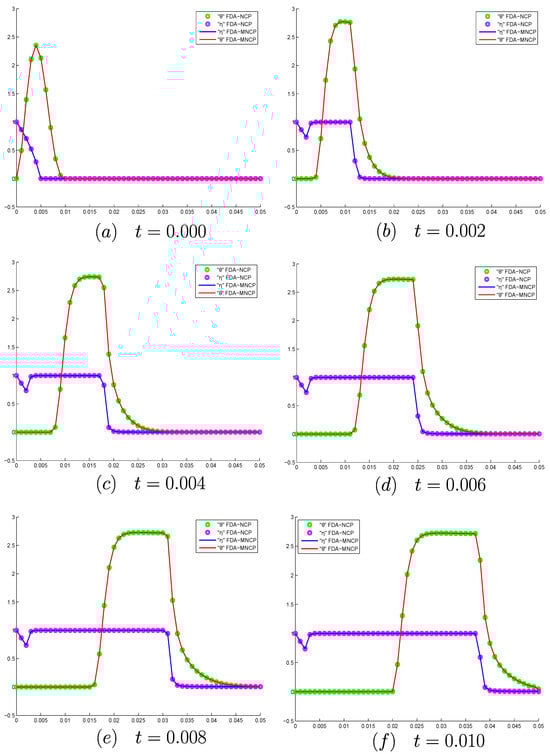
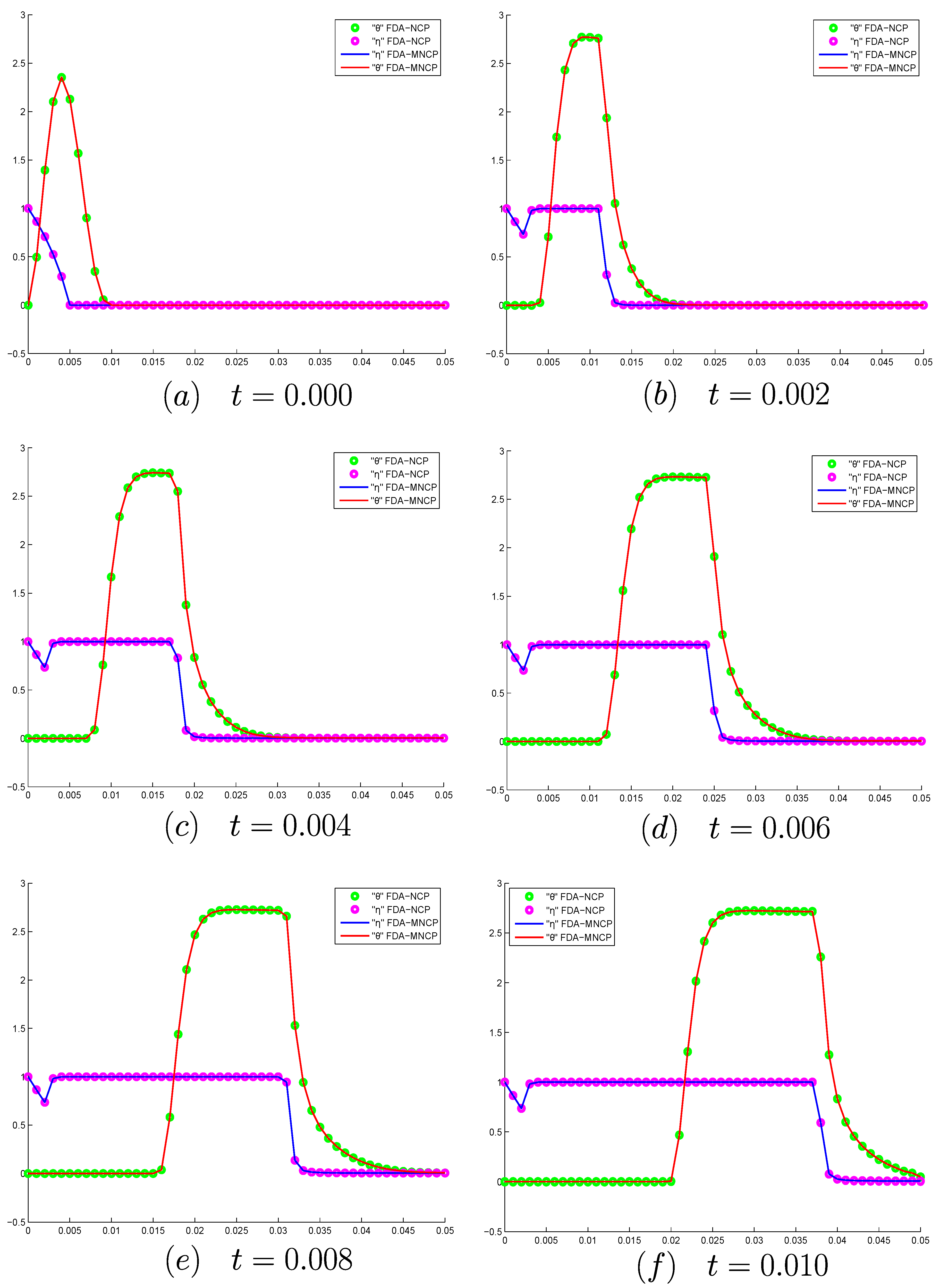
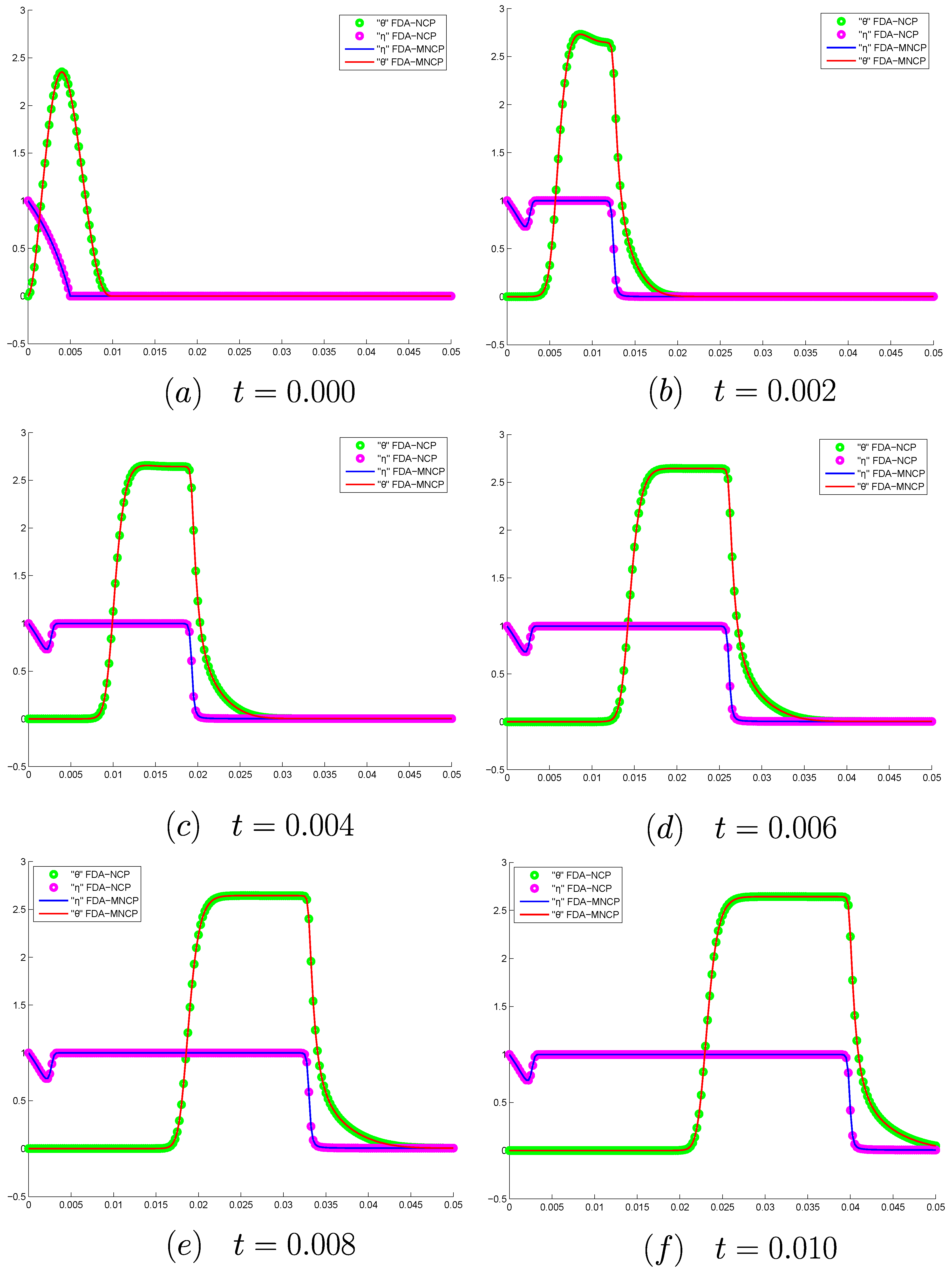
Figure 1. Comparison of the FDA-MNCP and FDA-NCP methods for M = 50 at time instants t = 0.000, 0.002, 0.004, 0.006, 0.008, 0.010. The values of $\theta$ are represented by green dots and a solid red line, and the values of $\eta$ are represented by pink dots and a solid blue line.

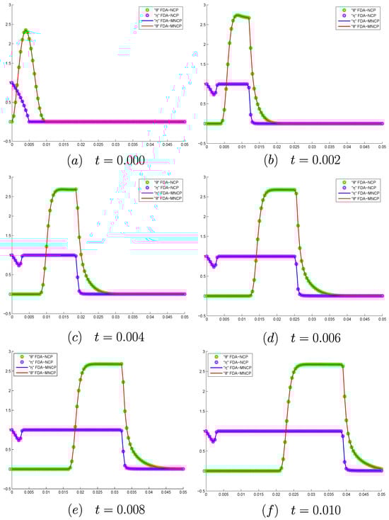
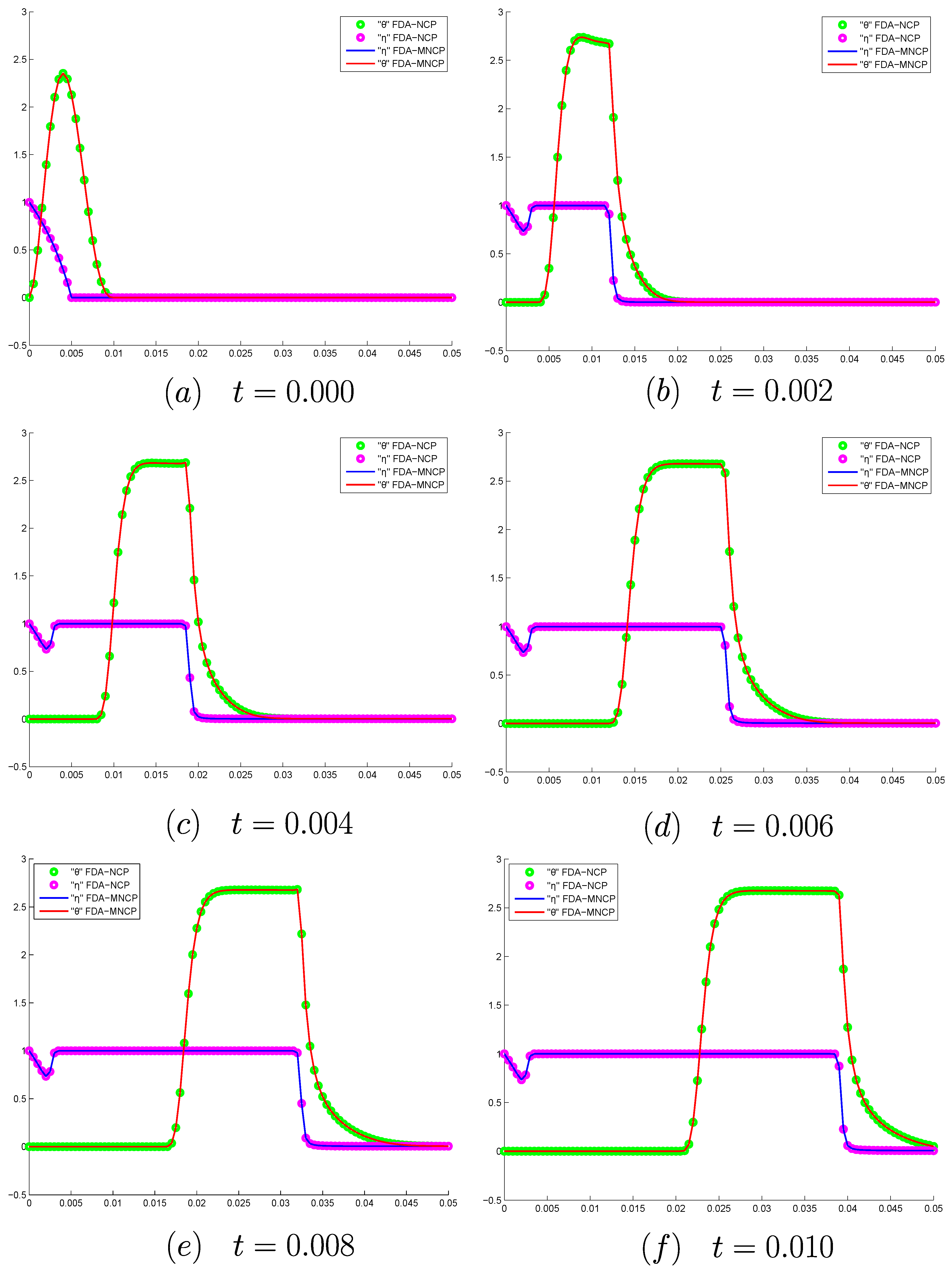
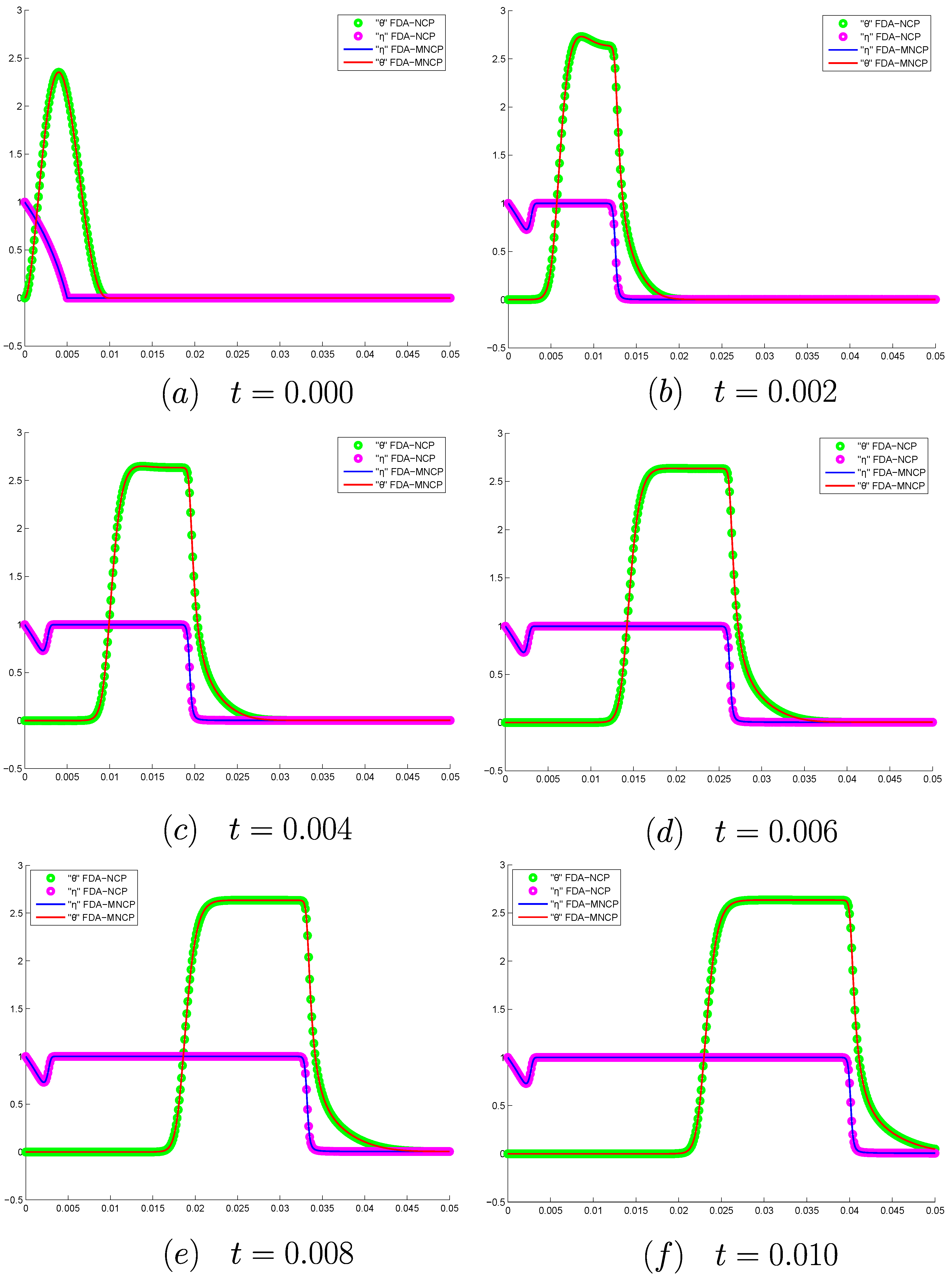
Figure 2. Comparison of the FDA-MNCP and FDA-NCP methods for M = 100 at times t = 0.000, 0.002, 0.004, 0.006, 0.008, 0.010. The values of $\theta$ are represented by green dots and a solid red line, and the values of $\eta$ are represented by pink dots and a solid blue line.

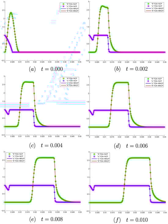
Figure 3. Comparison of the FDA-MNCP and FDA-NCP methods for M = 200 at times t = 0.000, 0.002, 0.004, 0.006, 0.008, 0.010. The values of $\theta$ are represented by green dots and a solid red line, and the values of $\eta$ are represented by pink dots and a solid blue line.

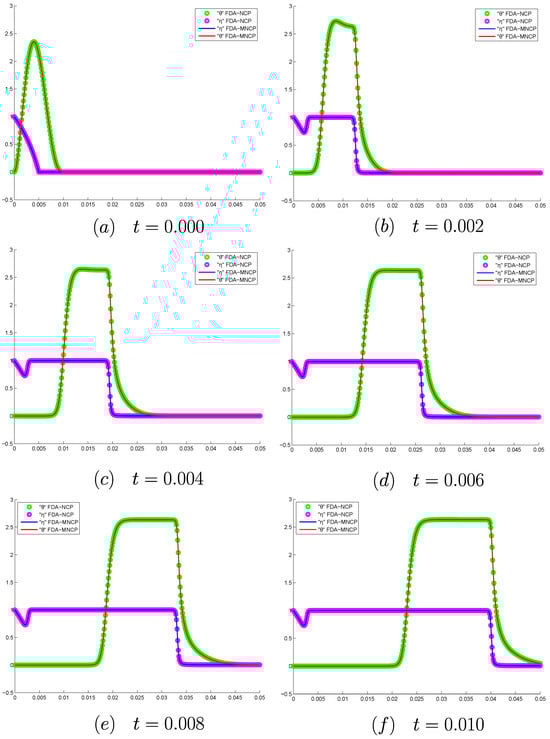
Figure 4. Comparison of the FDA-MNCP and FDA-NCP methods for M = 400 at times t = 0.000, 0.002, 0.004, 0.006, 0.008, 0.010. The values of $\theta$ are represented by green dots and a solid red line, and the values of $\eta$ are represented by pink dots and a solid blue line.

As shown in Figure 1, Figure 2, Figure 3 and Figure 4, the results obtained using the FDA-MNCP and FDA-NCP methods exhibit a strong agreement, as observed at the time instances indicated in the figures. In Figure 5, the differences between the two methods can be observed.

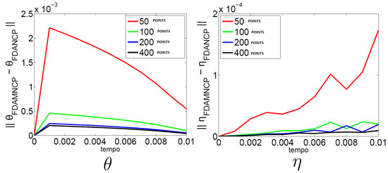
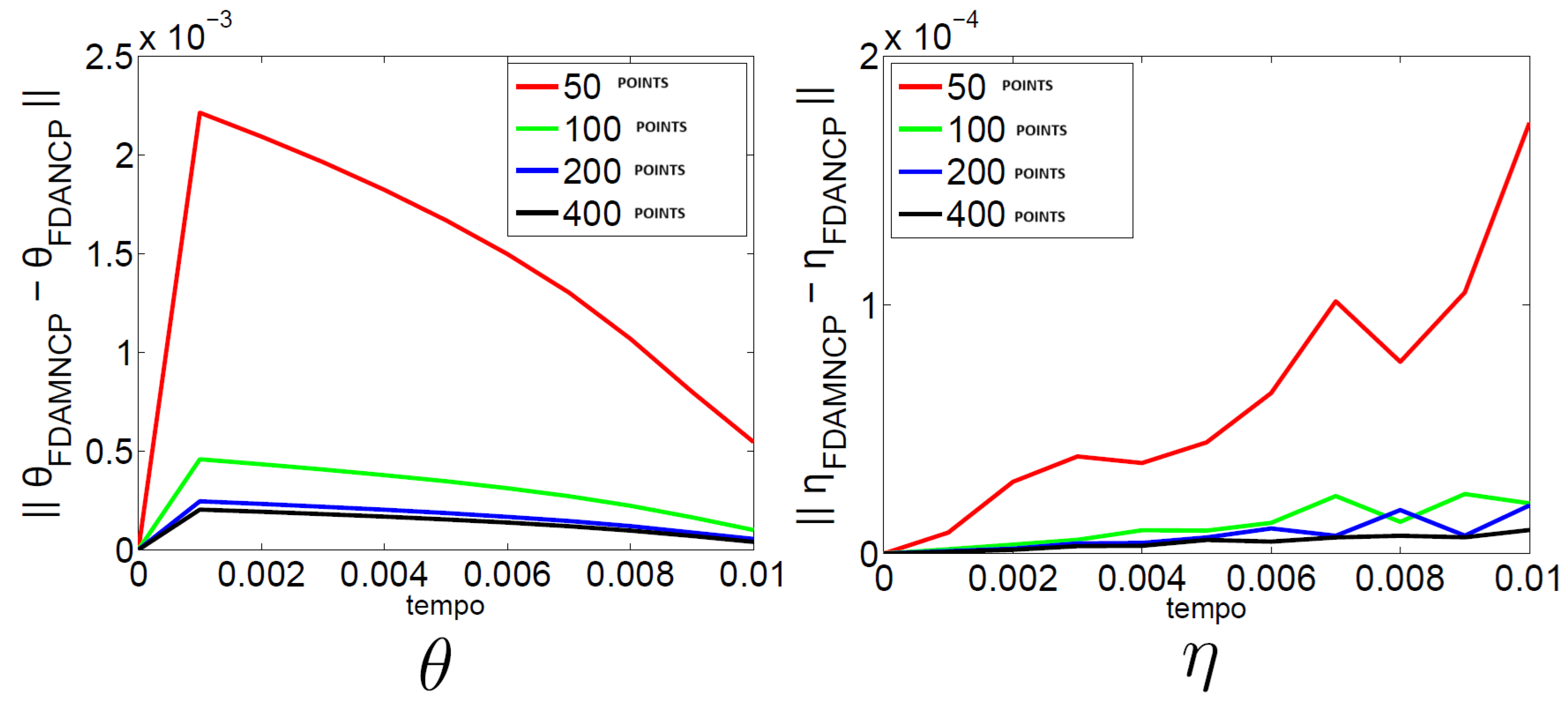
Figure 5. Difference between FDA-MNCP and FDA-NCP methods.

The differences between the solutions for $\theta$ and $\eta$ are very small as the number of points increases, demonstrating strong agreement between the FDA-MNCP and FDA-NCP methods [10].

Below, we present four tables comparing the computational time for $M=50,100,20,400$ using the FDA-MNCP method and the FDA-NCP method studied in [4].

As shown in Table 2, the computational time required by the FDA-MNCP method is approximately twice that of the FDA-NCP method when the x -axis is partitioned into 50 points. Additionally, the number of iterations for the FDA-MNCP method at the given time steps is higher than that of the FDA-NCP method. However, as the number of points in the mesh increases, the computational cost decreases. With 200 points, the cost is reduced by approximately $40\%$, and with 400, it is reduced by approximately $80\%$.

Table 2. Comparison of the computational process time with $M=50$ for the FDA-MNCP and FDA-NCP methods. $t\left(n\right)$ is the time measured in seconds that the method took to find the solution at time t.

	FDA-MNCP					FDA-NCP
$\mathit{t}$	$\mathit{t}\mathbf{\left(}\mathit{n}\mathbf{\right)}$	Iter	BL(t)	$\mathbf{\left[}\mathit{S}\mathbf{\right]}$	$\mathbf{[}\mathbf{\nabla }\mathit{S}\mathbf{]}$	$\mathit{t}\mathbf{\left(}\mathit{n}\mathbf{\right)}$	Iter	BL(t)	$\mathit{F}$	$\mathbf{\nabla }\mathit{F}$
0.001	0.401	33	1.0	43	34	0.194	20	1.0	43	40
0.002	0.411	34	0.8	44	35	0.194	20	1.0	43	40
0.003	0.406	34	1.0	43	35	0.199	20	1.0	43	40
0.004	0.386	32	0.8	41	33	0.184	20	1.0	43	40
0.005	0.385	32	0.8	41	33	0.178	21	1.0	45	42
0.006	0.406	34	0.8	43	35	0.198	21	1.0	45	42
0.007	0.395	33	0.8	42	34	0.193	21	1.0	45	42
0.008	0.403	33	0.8	43	34	0.229	21	1.0	45	42
0.009	0.390	32	0.8	42	33	0.169	21	1.0	45	42
0.010	0.405	33	0.8	44	34	0.173	21	1.0	45	42

In Table 3, we can also observe that the computational time required by the FDA-MNCP method is slightly higher than that of the FDA-NCP method, as is the number of iterations. However, as shown in the following tables, increasing the number of points in the spatial discretization leads to a reduction in the computational cost.

Table 3. Comparison of the computational process time with $M=100$ for the FDA-MNCP and FDA-NCP methods. t(n) is the time measured in seconds that the method took to find the solution at time t.

	FDA-MNCP					FDA-NCP
$\mathit{t}$	$\mathit{t}\mathbf{\left(}\mathit{n}\mathbf{\right)}$	Iter	BL(t)	$\mathbf{\left[}\mathit{S}\mathbf{\right]}$	$\mathbf{[}\mathbf{\nabla }\mathit{S}\mathbf{]}$	$\mathit{t}\mathbf{\left(}\mathit{n}\mathbf{\right)}$	Iter	BL(t)	$\mathit{F}$	$\mathbf{\nabla }\mathit{F}$
0.001	0.912	36	0.8	47	37	0.555	21	1.0	45	42
0.002	0.885	36	0.8	46	37	0.519	21	1.0	45	42
0.003	0.870	37	0.8	47	38	0.515	21	1.0	45	42
0.004	0.892	35	0.64	46	36	0.494	21	1.0	45	42
0.005	0.831	34	0.8	44	35	0.486	21	1.0	45	42
0.006	0.793	34	0.8	43	35	0.508	21	1.0	45	42
0.007	0.790	34	0.8	43	35	0.457	21	1.0	45	42
0.008	0.894	36	0.64	49	37	0.515	21	1.0	45	42
0.009	0.869	35	0.8	46	36	0.507	21	1.0	45	42
0.010	0.839	35	0.8	46	36	0.479	21	1.0	45	42

In Table 4, we observe that when the number of partitions is increased to 200, the computational time required by the FDA-MNCP method becomes shorter than that of the FDA-NCP method, although the number of iterations remains higher.

Table 4. Comparison of the computational process time with $M=200$ for the FDA-MNCP and FDA-NCP methods. t(n) is the time measured in seconds that the method took to find the solution at time t.

	FDA-MNCP					FDA-NCP
$\mathit{t}$	$\mathit{t}\mathbf{\left(}\mathit{n}\mathbf{\right)}$	Iter	BL(t)	$\mathbf{\left[}\mathit{S}\mathbf{\right]}$	$\mathbf{[}\mathbf{\nabla }\mathit{S}\mathbf{]}$	$\mathit{t}\mathbf{\left(}\mathit{n}\mathbf{\right)}$	Iter	BL(t)	$\mathit{F}$	$\mathbf{\nabla }\mathit{F}$
0.001	1.771	36	0.8	47	37	3.223	21	1.0	45	42
0.002	1.852	38	0.8	48	39	3.185	21	1.0	45	42
0.003	1.969	37	0.8	46	38	3.129	21	1.0	45	42
0.004	1.995	38	0.8	47	39	3.245	21	1.0	45	42
0.005	1.771	37	0.8	46	38	3.143	21	1.0	45	42
0.006	1.785	37	1.0	45	38	3.122	21	1.0	45	42
0.007	1.787	37	0.8	47	38	3.205	21	1.0	45	42
0.008	1.778	37	0.8	47	38	3.241	21	1.0	45	42
0.009	2.001	36	0.8	46	37	3.346	22	1.0	47	44
0.010	1.685	35	0.8	45	36	3.396	22	1.0	47	44

From Table 5, we observe that as the number of partitions increases significantly, the computational time required by the FDA-MNCP method becomes much lower than that of the FDA-NCP method [10]. This is because, in the FDA-MNCP method, the calculation of $\nabla S$ requires only half the computations compared to the calculation of $\nabla F$ in the FDA-NCP method [10], despite the higher number of iterations. Additionally, we note that the number of iterations remains relatively consistent across the previously presented tables.

Table 5. Comparison of the computational process time with $M=400$ for the FDA-MNCP and FDA-NCP methods. $t\left(n\right)$ is the time measured in seconds that the method took to find the solution at time t.

	FDA-MNCP					FDA-NCP
$\mathit{t}$	$\mathit{t}\mathbf{\left(}\mathit{n}\mathbf{\right)}$	Iter	BL(t)	$\mathbf{\left[}\mathit{S}\mathbf{\right]}$	$\mathbf{[}\mathbf{\nabla }\mathit{S}\mathbf{]}$	$\mathit{t}\mathbf{\left(}\mathit{n}\mathbf{\right)}$	Iter	BL(t)	$\mathit{F}$	$\mathbf{\nabla }\mathit{F}$
0.001	4.497	37	0.8	48	38	33.127	21	1.0	45	21
0.002	4.337	37	1.0	46	38	33.174	21	1.0	45	21
0.003	4.533	38	0.8	47	39	33.034	21	1.0	45	21
0.004	4.494	39	0.8	48	40	33.398	21	1.0	45	21
0.005	4.429	37	1.0	45	38	34.722	22	1.0	47	22
0.006	4.329	37	1.0	45	38	34.652	22	1.0	47	22
0.007	4.523	39	0.8	49	40	34.777	22	1.0	47	22
0.008	4.530	39	0.8	49	40	34.802	22	1.0	47	22
0.009	4.459	37	0.8	47	38	34.824	22	1.0	47	22
0.010	4.315	37	1.0	48	38	34.571	22	1.0	47	22

5. Error Analysis

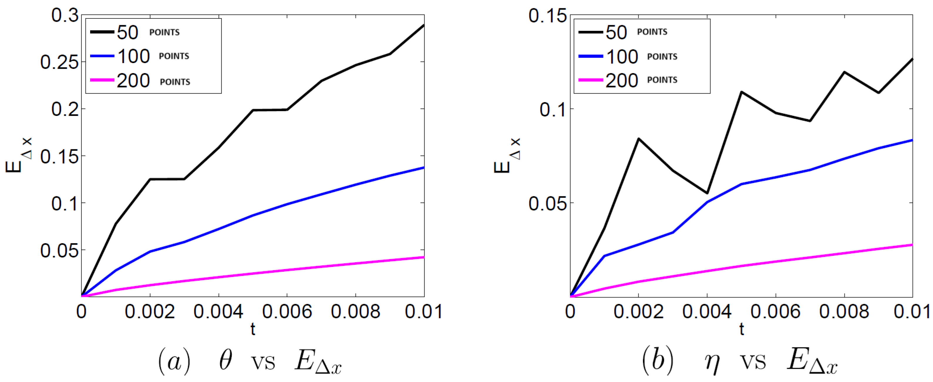
In this section, we describe the numerical study of the relative error for the FDA-MNCP method at each time step and for $E_{∆x}$, where $∆x=h,h/2,h/4$. The length of the time subinterval was kept constant at $∆t=k={10}^{-5}$ and $h={\displaystyle \frac{1}{50}}$, and the results were compared with those of the FDA-NCP method [4].

Table 6 and Table 8 present the relative error results for the FDA-MNCP method, while Table 7 and Table 9 show the relative error for the FDA-NCP method. These results are illustrated in Figure 6 and Figure 7.

Table 6. Relative error for $\theta$ with FDA-MNCP and $h={\displaystyle \frac{1}{50}}$ for the time instants t indicated in the first column.

t	${\mathit{E}}_{\mathit{h}}$	${\mathit{E}}_{\frac{\mathit{h}}{2}}$	${\mathit{E}}_{\frac{\mathit{h}}{4}}$	$\frac{{\mathit{E}}_{\mathit{h}}}{{\mathit{E}}_{\frac{\mathit{h}}{2}}}$	$\frac{{\mathit{E}}_{\frac{\mathit{h}}{2}}}{{\mathit{E}}_{\frac{\mathit{h}}{4}}}$
0.00100000	0.07757130	0.02809022	0.00730451	2.76	3.85
0.00200000	0.12495960	0.04805076	0.01233415	2.60	3.90
0.00300000	0.12512590	0.05824369	0.01679689	2.15	3.47
0.00400000	0.15843617	0.07200921	0.02080162	2.20	3.46
0.00500000	0.19817638	0.08645161	0.02467447	2.29	3.50
0.00600000	0.19866653	0.09841438	0.02840411	2.02	3.46
0.00700000	0.22936049	0.10892940	0.03195340	2.11	3.41
0.00800000	0.24606770	0.11916519	0.03538988	2.06	3.37
0.00900000	0.25789027	0.12872004	0.03877097	2.00	3.32
0.01000000	0.28886846	0.13735367	0.04209700	2.10	3.26

Table 7. Relative error for $\theta$ with FDA-NCP and $h={\displaystyle \frac{1}{50}}$ for the time instants t indicated in the first column.

t	${\mathit{E}}_{\mathit{h}}$	${\mathit{E}}_{\frac{\mathit{h}}{2}}$	${\mathit{E}}_{\frac{\mathit{h}}{4}}$	$\frac{{\mathit{E}}_{\mathit{h}}}{{\mathit{E}}_{\frac{\mathit{h}}{2}}}$	$\frac{{\mathit{E}}_{\frac{\mathit{h}}{2}}}{{\mathit{E}}_{\frac{\mathit{h}}{4}}}$
0.001	0.07753953	0.02808885	0.00730328	2.76	3.85
0.002	0.12490382	0.04804832	0.01233527	2.60	3.89
0.003	0.12507648	0.05824052	0.01679940	2.15	3.47
0.004	0.15841526	0.07200834	0.02080540	2.20	3.46
0.005	0.19818512	0.08645353	0.02467944	2.29	3.50
0.006	0.19869586	0.09841770	0.02841001	2.02	3.46
0.007	0.22940100	0.10893437	0.03196011	2.10	3.41
0.008	0.24613384	0.11917200	0.03539747	2.07	3.37
0.009	0.25797041	0.12872819	0.03877948	2.00	3.32
0.010	0.28897837	0.13736335	0.04210642	2.10	3.26

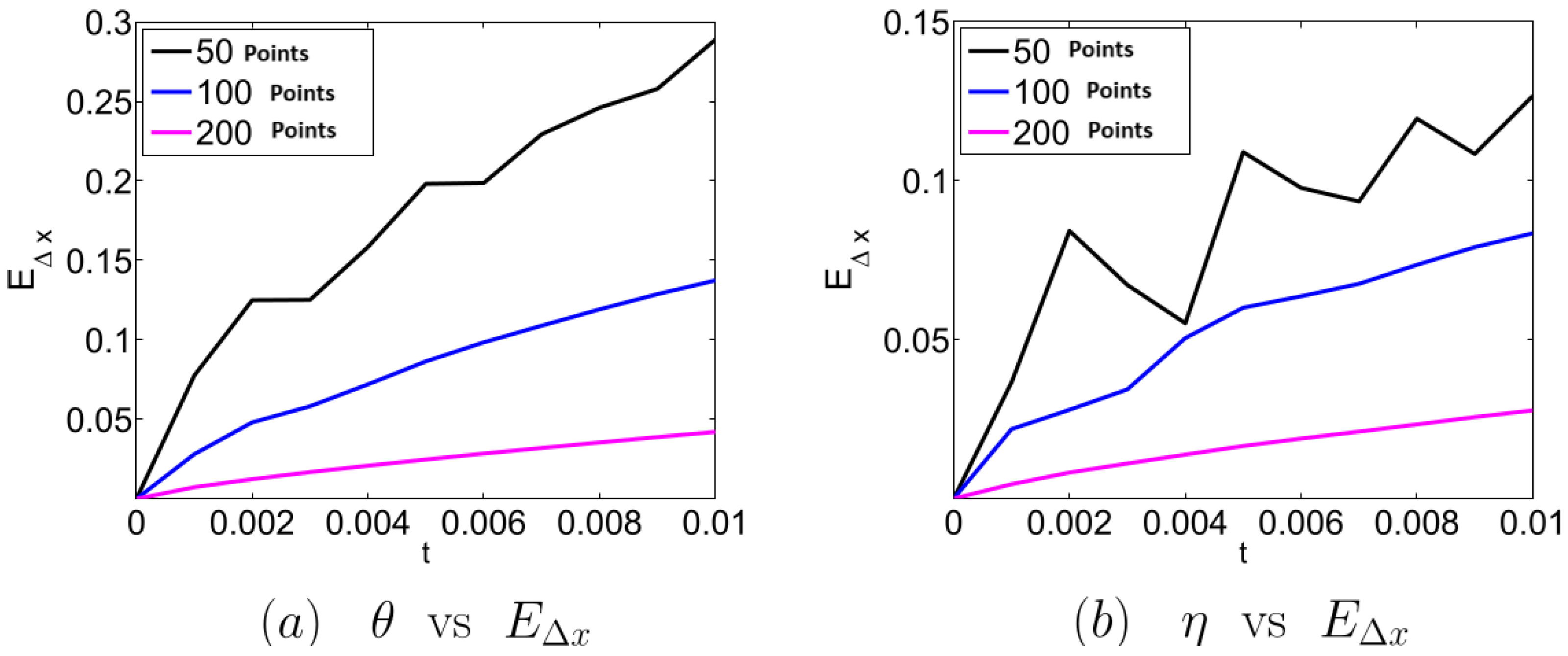
Figure 6. Time $\left(t\right)vs.E_{∆x}$. relative method error. Here, $∆x={\displaystyle \frac{1}{50}},{\displaystyle \frac{1}{100}},{\displaystyle \frac{1}{200}}$.

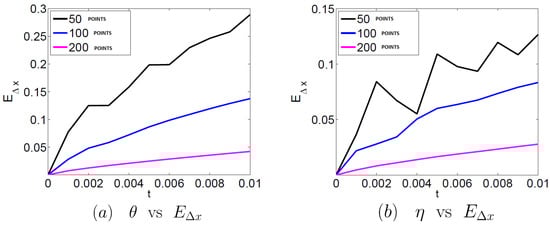
Figure 7. Time $\left(t\right)vs.E_{∆x}$. relative method error FDA-NCP. Here, $∆x={\displaystyle \frac{1}{50}},{\displaystyle \frac{1}{100}},{\displaystyle \frac{1}{200}}$.

As shown in Figure 6 and Figure 7, the relative errors for the FDA-MNCP and FDA-NCP methods are very similar. This is further confirmed by the following tables, which present the relative error for $\theta$ and $\eta$ using $h=1/50$.

In Table 6 and Table 7, we see that the relative errors $E_h,E_{\frac{h}{2}},E_{\frac{h}{4}}$ for $\theta$ of both the FDA-MNCP method and the FDA-NCP method are very similar since they are the same in the first three decimal places; that is, the error does not increase, but the computational cost is reduced as the points in the discretization increase.

Similarly, in Table 8 and Table 9 we see that $E_h,E_{\frac{h}{2}},E_{\frac{h}{4}}$ for $\eta$ of both the FDA-MNCP method and the FDA-NCP method are very similar, since the first three decimal places are the same.

Table 8. Relative error for $\eta$ with FDA-MNCP and $h={\displaystyle \frac{1}{50}}$ for the instants of time t indicated in the first column.

t	${\mathit{E}}_{\mathit{h}}$	${\mathit{E}}_{\frac{\mathit{h}}{2}}$	${\mathit{E}}_{\frac{\mathit{h}}{4}}$	$\frac{{\mathit{E}}_{\mathit{h}}}{{\mathit{E}}_{\frac{\mathit{h}}{2}}}$	$\frac{{\mathit{E}}_{\frac{\mathit{h}}{2}}}{{\mathit{E}}_{\frac{\mathit{h}}{4}}}$
0.00100000	0.03656879	0.02183277	0.00451877	1.67	4.83
0.00200000	0.08417410	0.02792488	0.00819559	3.01	3.41
0.00300000	0.06717364	0.03432880	0.01103677	1.96	3.11
0.00400000	0.05513563	0.05046208	0.01381861	1.09	3.65
0.00500000	0.10897196	0.06002542	0.01653614	1.82	3.63
0.00600000	0.09771893	0.06361601	0.01887177	1.54	3.37
0.00700000	0.09347666	0.06753455	0.02105732	1.38	3.21
0.00800000	0.11948456	0.07350345	0.02332175	1.63	3.15
0.00900000	0.10838295	0.07908666	0.02560247	1.37	3.09
0.01000000	0.12663557	0.08343716	0.02775604	1.52	3.01

Table 9. Relative error for $\eta$ with FDA-NCP and $h={\displaystyle \frac{1}{50}}$ for the instants of time t indicated in the first column.

t	${\mathit{E}}_{\mathit{h}}$	${\mathit{E}}_{\frac{\mathit{h}}{2}}$	${\mathit{E}}_{\frac{\mathit{h}}{4}}$	$\frac{{\mathit{E}}_{\mathit{h}}}{{\mathit{E}}_{\frac{\mathit{h}}{2}}}$	$\frac{{\mathit{E}}_{\frac{\mathit{h}}{2}}}{{\mathit{E}}_{\frac{\mathit{h}}{4}}}$
0.001	0.03656752	0.02183277	0.00451876	1.67	4.83
0.002	0.08415103	0.02792385	0.00819578	3.01	3.41
0.003	0.06714517	0.03432836	0.01103751	1.96	3.11
0.004	0.05513010	0.05046448	0.01382034	1.09	3.65
0.005	0.10898570	0.06002658	0.01653867	1.82	3.63
0.006	0.09776211	0.06361489	0.01887480	1.54	3.37
0.007	0.09351854	0.06753575	0.02106120	1.38	3.21
0.008	0.11952653	0.07350797	0.02332674	1.63	3.15
0.009	0.10846255	0.07909222	0.02560830	1.37	3.09
0.010	0.12671978	0.08344353	0.02776237	1.52	3.01

6. Conclusions

• We proposed solving the simple in situ combustion model using a numerical method based on an implicit finite difference scheme and a nonlinear mixed complementarity algorithm. We hypothesize that this approach may also be applicable to parabolic problems, which can be reformulated as mixed complementarity problems, as demonstrated for system (1).
• In this work, we demonstrated that the feasible interior point algorithm FDA-MNCP is an effective technique for numerically solving mixed complementarity problems.
• In the existing literature, the problem is formulated as a complementarity problem using two Hadamard products. However, this approach has the drawback of requiring the solution of large linear systems. In our formulation, only a single Hadamard product is used, resulting in smaller systems and, consequently, lower computational costs. This can be observed in the tables.
• We solved the in situ combustion model (1) using the nonlinear mixed complementarity algorithm and compared it to the FDA-NCP method. The results show that both solutions are very similar, as observed in Figure 1, Figure 2, Figure 3 and Figure 4. This suggests that the method can be applied to both parabolic and hyperbolic problems that can be formulated as mixed complementarity problems.
• The FDA-MNCP method has the advantage of supporting a larger number of spatial discretization points, as demonstrated in Table 4 and Table 5. It can also be observed that it is computationally faster than the FDA-NCP method when the spatial discretization is increased.
• Regarding the relative errors, Table 6 and Table 8 provide strong evidence of the convergence of the mixed complementarity algorithm applied to our formulation. This is further illustrated in Figure 5, which shows a reduction in linear growth as the mesh is refined.

References

- Chapiro, G.; Mazorche, S.R.; Herskovits, J.; Roche, J.R. Solution of the Non-linear Parabolic Problems using Nonlinear Complementarity Algorithm. (FDA-NCP). MecŃica Comput. 2010, 29, 2141–2153. [Google Scholar]
- Ferris, M.C.; Pang, J.S. Engineering and Economic Applications of Complementarity Problems; Society for Industrial and Applied Mathematics, SIAM: Philadelphia, PA, USA, 1997; Volume 39. [Google Scholar]
- Chapiro, G.; Mailybaev, A.A.; Souza, A.J.; Marchesin, D.; Bruining, J. Asymptotic approximation of long-time solution for low-temperature filtration combustion. Comput. Geosci. 2012, 16, 799–808. [Google Scholar]
- Ramirez Gutierrez, A. Application of the Nonlinear Complementarity Method for the Study of In Situ Oxygen Combustion. Master’s Thesis, Universidade Federal de Juis de Fora, Juiz de Fora, Brazil, 2013. [Google Scholar]
- Chapiro, G.; Ramirez, G.A.E.; Herkovits, J.; Mazorche, S.R.; Pereira, W.S. Numerical solution of a class of moving boundary problems with a nonlinear complementarity approach. J. Optim. Theory Appl. 2016, 168, 534–550. [Google Scholar]
- Bruining, J.; Marchesin, D.; Duijn, C.V. Steam injection into water-saturated porous rock. Comput. Appl. Math. 2003, 22, 359–395. [Google Scholar]
- Dake, L.P. Fundamentals of Reservoir Engineering; Elsevier: Amsterdam, The Netherlands, 1983. [Google Scholar]
- Burden, R.L.; Faires, J.D. Numerical Analysis, 9th ed.; Brooks/Cole—CENGAGE Learning: Boston, MA, USA, 2010. [Google Scholar]
- Dennis, J.E., Jr.; Schnabel, R.B. Numerical Methods for Unconstrained Optimization and Nonlinear Equations; Prentice-Hall: Hoboken, NJ, USA, 1983. [Google Scholar]
- Herskovits, J.; Mazorche, S. A feasible directions algorithm for nonlinear complementarity problems and applications in mechanics. Struct. Multidiscip. Otimiz. 2009, 37, 435–446. [Google Scholar]
- Serre, D. Systems of Conservation Laws 1. Hyperbolicity, Entropies, Shock Waves; Cambridge University Press: Cambridge, UK, 1999. [Google Scholar]
- Smoller, J. Shock Waves and Reaction-Diffusion Equations, 2nd ed.; Springer: Berlin/Heidelberg, Germany, 1994; 327p. [Google Scholar]
- Zeldovich, Y.B.; Barenblatt, G.I.; Librovich, V.B.; Makhviladze, G.M. The Mathematical Theory of Combustion and Explosion; Consultants Bureau: New York, NY, USA, 1985. [Google Scholar]
- Mayers, D.; Morton, K. Numerical Solution of Partial Differential Equations; Cambridge University Press: Cambridge, UK, 2005. [Google Scholar]
- Tannehill, J.C.; Anderson, D.A.; Pletcher, R.H. Computational Fluid Mechanics and Heat Transfer; Minkowycz, W.J., Sparrow, E.M., Eds.; CRC Press: Boca Raton, FL, USA, 1997. [Google Scholar]
Disclaimer/Publisher’s Note: The statements, opinions and data contained in all publications are solely those of the individual author(s) and contributor(s) and not of MDPI and/or the editor(s). MDPI and/or the editor(s) disclaim responsibility for any injury to people or property resulting from any ideas, methods, instructions or products referred to in the content. |
© 2025 by the authors. Licensee MDPI, Basel, Switzerland. This article is an open access article distributed under the terms and conditions of the Creative Commons Attribution (CC BY) license (https://creativecommons.org/licenses/by/4.0/).