Numerical Study of Flow Downstream a Step with a Cylinder Part 1: Validation of the Numerical Simulations

Abstract

The backward-facing step flow (BFSF) is a classical problem in fluid mechanics, hydraulic engineering, and environmental hydraulics. The nature of this flow, consisting of separation and reattachment, makes it a problem worthy of investigation. In this study, divided into two parts, the effect of a cylinder placed downstream of the step on the 2D flow structure was investigated. In Part 1, the classical 2D BFSF was validated by using OpenFOAM. The BFSF characteristics (reattachment, recirculation zone, velocity profile, skin friction coefficient, and pressure coefficient) were validated for a step-height Reynolds number in the range from 75 to 9000, covering both laminar and turbulent flow. The numerical results at different Reynolds numbers of laminar flow and four RANS turbulence models (standard k-ε, RNG k-ε, standard k-ω, and SST k-ω) were found to be in good agreement with the literature data. In laminar flow, the average error between the numerical results and experimental data for velocity profiles and reattachment lengths and the skin friction coefficient were lower than 8.1, 18, and 20%, respectively. In turbulent flow, the standard k-ε was the most accurate model in predicting pressure coefficients, skin friction coefficient, and reattachment length with an average error lower than 20.5, 17.5, and 6%, respectively. In Part 2, the effect on the 2D flow structure of a cylinder placed at different horizontal and vertical locations downstream of the step was investigated.

1. Introduction

The backward-facing step flow (BFSF) is one of the most important benchmarks in fluid mechanics. Moreover, due to the wake dynamics of the BFSF, it is considered to be an optimal separated flow geometry in hydraulic engineering and environmental hydraulics. Such a flow is characterized by flow separation and reattachment induced by a sharp expansion of the configuration [1]. It involves the most important features of a separated flow, such as free shear flow, separation and recirculation zone, reattachment, and redeveloping boundary layer. Such flow structures are presented in many applications, such as flow over aircraft and around buildings, flow in a bottom cavity, and stepped open channel flows. For environmental applications, the presence of the step at the bottom of rivers or lakes is of interest because of localized recirculation zones and transverse flows downstream of the step. One of the earliest attempts to study flow over a BFSF was done experimentally by Abbott and Kline [2]. Their results focused on the velocity profiles and the effects of different Reynolds numbers on flow properties. In particular, Armaly et al. [3], experimentally investigated the effect of step-height Reynolds number on flow separation by measurements of velocity distributions and the reattachment length over a wide range of Reynolds numbers (70 to 8000); hence, it covered laminar, transition, and turbulent regimes. In recent years, there have been many experimental studies carried out, with various BFS designs. It is widely acknowledged that the backward-facing step flow is controlled by the Reynolds number based on the step height (h) and the inlet velocity (U), the expansion ratio (ER) between the height of the outlet and the step of the channel, and the step angle.

It should be noted that the investigation of BFS flow from the laminar region to the turbulent region is different. The geometric parameters showed different effects on the flow separation and reattachment process. Many studies were focused on the reattachment length and the parametric effects on it, such as ER, and Reynolds number effect [4,5,6,7,8,9]. Flow behavior over BFS geometry for varying expansion ratios was investigated experimentally [6] to understand the flow separation and reattachment. The results showed that the primary recirculation length increased nonlinearly with an increasing expansion ratio at a constant Reynolds number. The effect of laminar Reynolds number for varying expansion ratios to understand the flow separation and reattachment by Biswas et al. [10]. The reattachment length increases with an increase in the expansion ratio and Reynolds numbers, whereas in turbulent flow such length is independent of the step-height Reynolds number for low expansion ratios and increases as the expansion ratio increases [6,11,12,13]. As such, many experimental [3,14,15,16,17,18,19,20,21] studies have been performed in laminar and turbulent regimes. Chen et al. [22] reviewed the recent theoretical, experimental, and numerical developments about BFSF. In addition to those theoretical challenges with the separation and reattachment length explained herein, there are also many issues with other features of the BFS study, such as wall pressure coefficient and skin friction. It is generally reported that both the pressure coefficient (C_p) and skin friction coefficient (C_f) show a drop near the step and then gradually increase again in the downward flow. The skin friction coefficient (C_f) is strongly dependent on the step-height Reynolds number [16].

During the last several decades, computer simulations of physical processes have been used in scientific research and the analysis and design of engineered systems. Several computational studies [10,23,24,25,26,27,28,29,30,31,32,33,34,35] have been performed to examine the influence of backward-facing step geometry in laminar and turbulent regimes. Two-equation eddy-viscosity models appear to be preferred among turbulence models because they incorporate significantly more turbulence physics and less special empiricism than algebraic models while avoiding numerical implementation difficulties and excessive computational cost when compared to other more complex models [36]. For a long time, various RANS turbulence models were used for investigating two-dimensional separating and reattaching flow [37].

One conventional approach is to solve the Reynolds-averaged Navier–Stokes (RANS) equations, such as the widely used k-ε model. Some research has been done on different turbulence models about the reattachment length of backward-facing step flow [29,36,38,39,40]. Recently, Wang et al. [41] used k-ε and LES models for a backward-facing step at Reynolds number 9000. The results showed that the LES model could not effectively simulate the boundary layer near the wall areas without extremely fine mesh, and it tends to overestimate separation at the top wall. These resulted in static pressure, mean velocity, and turbulent kinematic energy showing a larger peak value when compared to other methods.

The flow past a cylinder is a classical benchmark in fluid mechanics. In fluid mechanics, the interactions of step and cylinder are of interest because the flow over a backward-facing step could be controlled by using additional elements like a cylinder. In environmental applications, cylindrical obstacles such as large wood may be trapped near the step, altering the turbulent properties of the flow. In this study, divided into two parts, the effect of a cylinder placed downstream of the step on the 2D flow structure was investigated. In Part 1, the classical 2D BFSF was validated, and in Part 2, the effect on the 2D flow structure of a cylinder placed at different horizontal and vertical locations downstream of the step was studied.

Nowadays, numerical simulation is used to solve problems not only to find a solution but also to ensure quality. Validation is the assessment of the accuracy and reliability of a computational simulation by comparison with experimental data [42,43]. In the present study, two-dimensional numerical simulations were performed by using the open-source code Open-Source Field Operation and Manipulation (OpenFOAM). The study is divided into two parts. Part 1 presents a 2D validation procedure for CFD simulations of a backward-facing step flow (BFSF). The flow characteristics such as reattachment, recirculation zone, velocity profile, skin friction coefficient, and pressure coefficient were validated for a step height-based Reynolds number in the laminar and turbulent flow. Moreover, four RANS turbulence models, such as standard k-ε, RNG k-ε, standard k-ω, and SST k-ω were comparatively evaluated. Part 1 is organized as follows: Section 2 reports the numerical methodology including geometry and mesh generation. In addition, the governing equations, boundary conditions, and numerical schemes are presented for laminar and turbulent. Section 3 reports comparison results of the present numerical simulation, such as reattachment length, recirculation zone, velocity profile, skin friction, and pressure coefficient, with literature experimental data and numerical results. The results of the validation are summarized in Section 4. Finally, the conclusions are presented in Section 5.

In Part 2, the two-dimensional classical BFSF geometry was modified by adding a cylinder placed at different locations downstream of the step. The flow structure in such modified BFSF was investigated in both laminar and turbulent regimes.

2. Set-Up of the Numerical Simulations

Computational fluid dynamics (CFD) is increasingly used to study a wide variety of complex environmental fluid mechanics (EFM) processes. However, the accuracy and reliability of CFD modeling and the correct use of CFD results can easily be compromised [44]. Numerical simulations were performed by using the open-source code OpenFOAM v 2112. The OpenFOAM is a software based on a finite volume approach. In the present study, several numerical simulations were performed. The overall steps of numerical modeling of this study are illustrated in Figure 1.

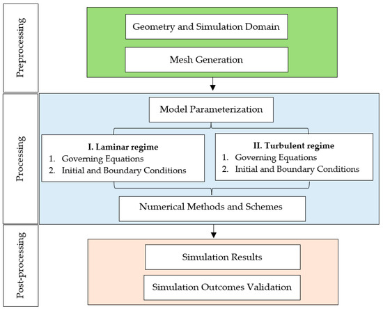
Figure 1. Flowchart of the numerical modeling procedures.

2.1. Geometry and Simulation Domain

In Part 1, for validation, we consider a two-dimensional, classically backward-facing step flow, namely BFSF 1. The geometry was considered by following the geometry experimentally studied by Armaly et al. [3] and Wang et al. [1] with an expansion ratio (ER = h₂/h₁ = 2). The computational domain of the present study consists of a total longitudinal length of 56h (L_u = 6h, L_d = 50h, and L_u and L_d are, respectively, the length upstream and downstream of the step). Based on Biswas et al. [10], a distance of five times the channel height upstream of the step (Lu ≥ 5h₁, h₁ = h) was verified to be sufficient. At the outlet of the computational domain, the flow was fully developed. The sketch of the BFSF is presented in Figure 2.

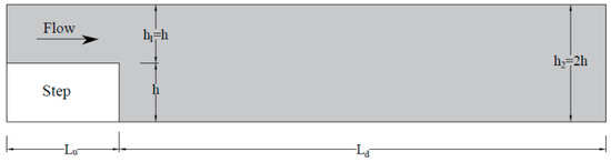
Figure 2. Schema of backward-facing step flow (BFSF) (not to scale).

2.2. Mesh Generation

During the preprocessing phase of the CFD modeling, the geometry and domain for the mesh were created. In OpenFOAM, geometries for internal flows are typically created by using a meshing tool known as blockMesh, which creates fully structured hexahedral meshes. In this study, the structured rectangular hexahedral mesh was considered. Structured meshing is generally more straightforward to implement, faster to execute, and tends to be more accurate than unstructured ones [45]. Moreover, structured meshes require more regular memory access; consequently, the latency during simulations is lower [46]. To ensure the validity and accuracy of the solution scheme, several grid sizes were examined. Mesh independence was assessed and validated by using experimental data. Meshes of different sizes were applied, and the reattachment lengths were compared to the corresponding experimental data [1]. The sensitivity of the model to certain parameters was extensively discussed. The test of the grid independence was performed by computing the dimensionless reattachment length Lr/h, in a Re_h = 544 for five different grids (see Table 1). It was found that the computed results were independent of the number of grid points and the relative error between the third and the fourth grid was very small and could be neglected to decrease effort and computational time. Given the accuracy and duration of the computation, a total number of 129200 cells were selected.

Table 1. Grid independence test results.

Grid No.	Number of Cells	Lr/h	Differences with Experimental Data
Mesh 1	86,000	10.77	22.95%
Mesh 2	95,200	11.2	19.9%
Mesh 3	104,000	11.5	17.76%
Mesh 4	129,200	11.81	15.56%
Mesh 5	132,000	11.82	15.49%

The cell size near the walls and step was fine to have enough resolution. The mesh was gradually refined toward the bottom and step, as shown in Figure 3, to enhance the accuracy near the bottom wall to ensure that the dimensionless distance (y+) remained within the viscous sublayer. In addition, the mesh was refined near the cylinder to properly resolve the separation of boundary layers.

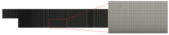
Figure 3. General view of the grid and zoom of the grid near the bottom wall.

2.3. Model Parameterization

For the simulation, water with density ρ = 997 Kg/m³ and dynamic viscosity (μ) 8.905 × 10⁻⁴ N·s/m² was selected as fluid. The Reynolds number based on the step height (h) was defined as ${\mathrm{Re}}_{\mathrm{h}}= \frac{\mathrm{Uh}}{\mathsf{\upsilon }}$. According to Armaly et al. [3], in the BFSF, the laminar regime occurs for step-height Reynolds numbers Re_h < 900, the transitional regime is in the range 900 < Re_h < 4950 and the turbulent regime is Re_h > 4950. The present study was carried out in the Reynolds number range covering laminar and turbulent flows. Table 2 lists the values of Reynolds numbers that were tested in this study.

Table 2. Range of Reynolds numbers based on step height (Re_h) for the classical backward-facing step flow with an expansion ratio (ER = h₂/h₁ = 2) in laminar flow.

Reh (Step Height)	75	158	336	420	544	672	755
Run	BFSF 1–L1	BFSF 1–L2	BFSF 1–L3	BFSF 1–L4	BFSF 1–L5	BFSF 1–L6	BFSF 1–L7

2.4. Laminar Flow

2.4.1. Governing Equations

Continuity and momentum equations for two-dimensional (2D) flow in the laminar regime for an incompressible isothermal fluid (with constant density) can be written as:

Mass equation	$\frac{\partial \mathrm{u}}{\partial \mathrm{x}}+\frac{\partial \mathrm{v}}{\partial \mathrm{y}}=0$	(1)
Momentum equation	$\left(\frac{\partial \mathrm{u}}{\partial \mathrm{t}}+\mathrm{u}\frac{\partial \mathrm{u}}{\partial \mathrm{x}}+\mathrm{v}\frac{\partial \mathrm{u}}{\partial \mathrm{y}}\right)={ \mathrm{g}}_{\mathrm{x}}- \frac{1}{\rho }\frac{\partial \mathrm{p}}{\partial \mathrm{x}}+\mathsf{\upsilon }\left(\frac{{\partial }^2\mathrm{u}}{\partial {\mathrm{x}}^2}+\frac{{\partial }^2\mathrm{u}}{\partial {\mathrm{y}}^2}\right)$ $\left(\frac{\partial \mathrm{v}}{\partial \mathrm{t}}+\mathrm{u}\frac{\partial \mathrm{v}}{\partial \mathrm{x}}+\mathrm{v}\frac{\partial \mathrm{v}}{\partial \mathrm{y}}\right)={ \mathrm{g}}_{\mathrm{y}}-\frac{1}{\rho }\frac{\partial \mathrm{p}}{\partial \mathrm{y}}+\mathsf{\upsilon }\left(\frac{{\partial }^2\mathrm{v}}{\partial {\mathrm{x}}^2}+\frac{{\partial }^2\mathrm{v}}{\partial {\mathrm{y}}^2}\right)$,	(2)

where υ is kinematic viscosity, p is the pressure, u and v are velocity components in the x and y directions, and g is the acceleration of gravity.

2.4.2. Initial and Boundary Conditions

Boundary conditions were assigned at the inlet, the outlet, and the walls. A parabolic velocity profile was assigned to the inlet. A summary of these boundary conditions which were used for the laminar regime is given in Table 3.

Table 3. Boundary conditions of the backward-facing step in the laminar regime.

Boundary Type Description	Inlet	Outlet	Wall (Upper Wall, Bottom Wall)
Pressure (p)	zeroGradient	fixedValue	zeroGradient
Velocity (u)	fixedValue	zeroGradient	noSlip

2.5. Turbulent Flow

2.5.1. Governing Equations and Turbulence Modeling

The most widely applied approach to simulate a turbulent flow is based on the time averaging, herein Reynolds-averaging, of the Navier–Stokes equations, leading to the Reynolds-averaged N-S (RANS) equations. OpenFOAM offers a large range of methods and models to simulate the turbulence, including the RANS. RANS mass and momentum conservation laws for two-dimensional flow for an incompressible isothermal fluid (with constant density) can be written as

Mass equation	$\frac{\partial \overline{\mathrm{u}}}{\partial \mathrm{x}}+\frac{\partial \overline{\mathrm{r}}}{\partial \mathrm{y}}=0$	(3)
Momentum equation	$\frac{\partial \overline{\mathrm{u}}}{\partial \mathrm{t}}+\overline{\mathrm{u}}\frac{\partial \overline{\mathrm{u}}}{\partial \mathrm{x}}+\overline{\mathrm{v}}\frac{\partial \overline{\mathrm{u}}}{\partial \mathrm{y}}={ \mathrm{g}}_{\mathrm{x}}-\frac{1}{\rho }\frac{\partial \overline{\mathrm{p}}}{\partial \mathrm{x}}+\mathsf{\upsilon }{\nabla }^2\overline{\mathrm{u}}+\frac{\partial }{\partial \mathrm{x}}\left({\mathsf{\upsilon }}_{\mathrm{t}}\frac{\partial \overline{\mathrm{u}}}{\partial \mathrm{x}}\right)+\frac{\partial }{\partial \mathrm{y}}\left({\mathsf{\upsilon }}_{\mathrm{t}}\frac{\partial \overline{\mathrm{u}}}{\partial \mathrm{y}}\right)$ $\frac{\partial \overline{\mathrm{u}}}{\partial \mathrm{t}}+\overline{\mathrm{u}}\frac{\partial \overline{\mathrm{u}}}{\partial \mathrm{x}}+\overline{\mathrm{v}}\frac{\partial \overline{\mathrm{u}}}{\partial \mathrm{y}}={ \mathrm{g}}_{\mathrm{x}}-\frac{1}{\rho }\frac{\partial \overline{\mathrm{p}}}{\partial \mathrm{x}}+\mathsf{\upsilon }{\nabla }^2\overline{\mathrm{u}}+\frac{\partial }{\partial \mathrm{x}}\left({\mathsf{\upsilon }}_{\mathrm{t}}\frac{\partial \overline{\mathrm{u}}}{\partial \mathrm{x}}\right)+\frac{\partial }{\partial \mathrm{y}}\left({\mathsf{\upsilon }}_{\mathrm{t}}\frac{\partial \overline{\mathrm{u}}}{\partial \mathrm{y}}\right)$,	(4)

where $\overline{\mathrm{p}}$ is the mean fluid pressure, $\overline{\mathrm{u}}$ and $\overline{\mathrm{v}}$ are the mean velocity components, and υ_t is the turbulent eddy kinematic viscosity.

The simplest RANS models are based on the concept of the eddy viscosity (υ_t) introduced by Boussinesq in 1887 [47], giving a relation between the Reynolds stress tensor and the average velocity gradient tensor [48]. Different turbulence models estimate υ_t based on different turbulent variables. In this study, four RANS turbulence models, such as standard k-ε, RNG k-ε, standard k-ω, and SST k-ω were comparatively applied.

The standard k-ε model is the most widely applied turbulence model. It is a two-equation model that includes two extra transport equations to represent the turbulent properties of the flow: the turbulent kinetic energy (k) and the turbulent energy dissipation (ε), together with a specification for the eddy viscosity (υ_t). Its formulation is presented as

$$\frac{\partial \mathrm{k}}{\partial \mathrm{t}}+{\overline{\mathrm{u}}}_{\mathrm{j}}\frac{\partial \mathrm{k}}{\partial {\mathrm{x}}_{\mathrm{j}}}=\frac{\partial }{\partial {\mathrm{x}}_{\mathrm{j}}}\left[\left(\mathsf{\upsilon }+\frac{{\mathsf{\upsilon }}_{\mathrm{t}}}{{\mathsf{\sigma }}_{\mathrm{k}}}\right)\frac{\partial \mathrm{k}}{\partial {\mathrm{x}}_{\mathrm{j}}}\right]-{\mathsf{\upsilon }}_{\mathrm{t}}\frac{\partial {\overline{\mathrm{u}}}_{\mathrm{i}}}{\partial {\mathrm{x}}_{\mathrm{j}}}\left(\frac{\partial {\overline{\mathrm{u}}}_{\mathrm{i}}}{\partial {\mathrm{x}}_{\mathrm{j}}}+\frac{\partial {\overline{\mathrm{u}}}_{\mathrm{j}}}{\partial {\mathrm{x}}_{\mathrm{i}}}\right)-\mathsf{\epsilon }$$

(5)

$$\frac{\partial \mathsf{\epsilon }}{\partial \mathrm{t}}+{\overline{\mathrm{u}}}_{\mathrm{j}}\frac{\partial \mathsf{\epsilon }}{\partial {\mathrm{x}}_{\mathrm{j}}}-\frac{\partial }{\partial {\mathrm{x}}_{\mathrm{j}}}\left[\left(\mathsf{\upsilon }+\frac{{\mathsf{\upsilon }}_{\mathrm{t}}}{{\mathsf{\sigma }}_{\mathsf{\epsilon }}}\right)\frac{\partial \mathsf{\epsilon }}{\partial {\mathrm{x}}_{\mathrm{j}}}\right]={\mathrm{C}}_1\frac{\mathsf{\epsilon }}{\mathrm{k}}{\mathsf{\upsilon }}_{\mathrm{t}}\frac{\partial {\overline{\mathrm{u}}}_{\mathrm{i}}}{\partial {\mathrm{x}}_{\mathrm{j}}}\left(\frac{\partial {\overline{\mathrm{u}}}_{\mathrm{i}}}{\partial {\mathrm{x}}_{\mathrm{j}}}+\frac{\partial {\overline{\mathrm{u}}}_{\mathrm{j}}}{\partial {\mathrm{x}}_{\mathrm{i}}}\right)-{\mathrm{C}}_2\frac{{\mathsf{\epsilon }}^2}{\mathrm{k}}$$

(6)

$${\mathsf{\upsilon }}_{\mathrm{t}}={\mathsf{\rho }\mathrm{C}}_{\mathsf{\mu }}\frac{\mathrm{k}}{\mathsf{\epsilon }},$$

(7)

where k is turbulent kinetic energy, and ε is the turbulent kinetic energy dissipation rate, whereas C₁, C₂, C_µ, σ_k, and σ_ɛ are constants, and their values are listed in Table 4 [49].

Table 4. Values of the constants of the standard k-ε model.

C1	C2	Cµ	σk	σɛ
1.44	1.92	1.3	1	1.3

The RNG k-ε model was developed by using renormalization group (RNG) methods by Yakhot et al. [50] to renormalize the Navier–Stokes equations. The RNG version adds a term for the ɛ equation, which is known to be responsible for differences in its performance. It is a two-equation transport model for k and ε. The RNG k-ε model formulation differs from that of the standard k-ɛ in the values of the parameters. The standard k-ω model is a two-equation model developed by Wilcox [51] with an approach similar to the k-ε model. It applies the same expression for the turbulent kinetic energy k but it considers the rate of dissipation of energy per unit volume and time, called the specific dissipation rate ω, instead of the turbulent energy dissipation (ε). In the k-ω model, the turbulent viscosity is computed by

$${\mathsf{\upsilon }}_{\mathrm{t}}=\frac{\mathrm{k}}{\mathsf{\omega }}.$$

(8)

The shear stress transport (SST) k-ω model is a two-equation eddy-viscosity model. It is similar to the standard k-ω although the former includes several improvements and other constant variables. It is a hybrid model combining the k-ω and the k-ε models. This method effectively blends the accurate formulation of the k-ω model in the near-wall region with the free-stream independence of the k-ε model in the far-field region, away from the wall. The SST formulation switches to a k-ε behavior in the freestream and thereby avoids the common k-ω problem that the model is too sensitive to the inlet free-stream turbulence properties.

2.5.2. Initial and Boundary Conditions

In turbulent flow, the standard k-ε, RNG k-ε, standard k-ω, and SST k-ω turbulence models were employed. The Reynolds number based on the step height (h) was Re_h = 9000. Table 5 lists all runs in turbulent flow over backward-facing step flow.

Table 5. Runs of turbulent flow over the classical backward-facing step at different turbulence models.

Run	Reh (Step Height)	Turbulence Model
BFSF 1–T1	9000	Standard k-ε
BFSF 1–T2	9000	RNG k-ε
BFSF 1–T3	9000	Standard k-ω
BFSF 1–T4	9000	SST k-ω

The initial values of turbulent kinetic energy (k) and dissipation rate (ε) can be estimated by [49]

$$\mathrm{k}=\frac{3}{2} {\left(\left|{\mathrm{u}}_{\mathrm{reff}}\right|{\mathrm{T}}_{\mathrm{i}}\right)}^2$$

(9)

$$\mathsf{\epsilon }=\frac{{0.09}^{0.75}{\mathrm{k}}^{1.5}}{\mathrm{l}},$$

(10)

where u_reff is the inlet flow velocity, l = 0.07L (L is the characteristic inlet scale (m)), and T_i is the turbulent intensity (5%). In omega-based models, the initial value of the specific dissipation rate ω can be estimated by

$$\mathsf{\omega }=\frac{{\mathrm{k}}^{0.5}}{{0.09}^{0.25}\mathrm{l}}.$$

(11)

Initial values for pressure (p = 0) and velocity (U = 0.801 m/s) were used. In addition, the initial values of turbulence quantities were calculated by using Equations (9)–(11), where k = 0.002406 m²/s², ɛ = 0.0277 m²/s³, and ω = 124.82 l/s.

Boundary conditions were assigned at the inlet, the outlet, and the walls. In the turbulent regime, several boundary conditions were required. A summary of these boundary conditions, which were used for the turbulent regime, is given in Table 6.

Table 6. Boundary conditions of the backward-facing step in the turbulent regime.

Boundary Type Description		Inlet	Outlet	Upper Wall/Bottom Wall
Pressure	P (kg/s·m2)	zeroGradient	fixedValue	zeroGradient
Velocity	u (m/s)	fixedValue	inletOutlet	noSlip
Turbulence qantities	k (m2/s2)	fixedValue	zeroGradient	kqRWallFunction
	ε (m2/s3)	fixedValue	zeroGradient	epsilonWallFunction
	ω (1/s)	fixedValue	zeroGradient	omegaWallFunction

2.5.3. Numerical Methods and Numerical Schemes

The governing equations were discretized based on the finite-volume method (FVM). The numerical integration was conducted by using the pressure-implicit with splitting of operators (PISO) algorithm. PISO is a pressure-velocity calculation procedure for the Navier–Stokes equations. The time term was discretized by using second-order backward and Euler schemes. In the laminar regime, the terms of the equations are discretized by using a Gaussian linear scheme in all cases. However, the discretization schemes for the turbulence kinetic energy (k), turbulent kinetic energy dissipation rate (ε), and specific dissipation rate (ω) were implemented by using a Gaussian upwind scheme. The transient solvers icoFoam and pisoFoam were used for the laminar and turbulent flow, respectively. To ensure convergence to the numerical solutions, all residuals were required to be dropped below a value of 10⁻⁶. Moreover, to ensure the stability of simulations, time steps were automatically modified, so that maximum Courant numbers always remained below 0.8.

3. Results

3.1. Laminar Flow

3.1.1. Recirculation Zone and Reattachment Length

The most important characteristics of the backward-facing step flow are flow separation and reattachment. The adverse pressure gradient due to the sudden expansion at the edge of the step, induced flow separation. A sketch of the 2D backward-facing step flow is shown in Figure 4.

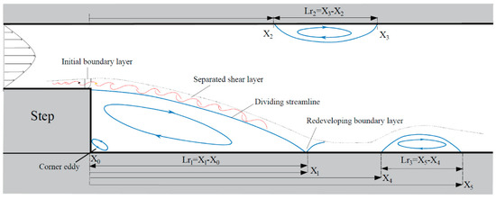
Figure 4. Sketch of the flow over the backward-facing step.

In the classical BFSF, the flow pattern involves several different flow regions: initial boundary layer, separated free shear layer, corner eddy, primary recirculation zone on the bottom wall, second recirculation zone on the upper wall, redeveloping boundary layer, and third recirculation zone on the bottom wall, as shown in Figure 4. The physics of separation regions could be described as follows: flow separated at the step (X₀) and reattached to the bottom wall (X₁). This is the primary recirculation zone having a length of Lr₁, which increased as Re_h increased. In addition to the primary recirculation zone (Lr₁), a second recirculation zone (Lr₂) near the upper wall for Re_h > 300 was reported in previous studies [3]. Point X₂ shows the starting location of the second recirculation zone and point X₃ is its corresponding end on the upper wall. Erturk [25] found that with an expansion ratio of 2 for Re_h > 1275, a third recirculating zone (Lr₃) was observed between points X₄ and X₅ with length Lr₃. Its length Lr₃ increased as Re_h increased. However, Armaly et al. [3] found that the third recirculation region (Lr₃) was in the early part of the transitional flow, and it was not observed for Re_h > 1725. Cherdron et al. [52] and Sparrow and Kaljes [53] suggested that the third recirculation zone was caused by vortex shedding from the edge of the step. These vortices were thought to approach the wall, and the third recirculation zone might be due to the sharp change of flow direction that eddies experience [3]. Table 7 lists the value of the normalized location of starting and ending recirculation zones in the BFSF.

Table 7. The reattachment and separation points of the recirculation zones vs. Re_h in laminar flow.

Run	BFSF 1–L1	BFSF 1–L2	BFSF 1–L3	BFSF 1–L4	BFSF 1–L5	BFSF 1–L6	BFSF 1–L7
X1/h	2.88	5.25	9.15	10.4	11.5	12.5	13.37
X2/h	-	-	7.8	8.65	8.9	10.2	10.62
X3/h	-	-	10.65	14.15	18.6	21.5	23.1

Figure 5 compares the primary recirculation zone (Lr₁) with experimental data of Armaly et al. [3], Lee and Mateescu [14], and Tihon et al. [19], as well as numerical studies of Gualtieri [23] and Erturk [25].

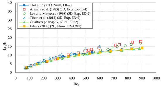
Figure 5. Dimensionless primary reattachment length Lr₁/h vs. Re_h in laminar flow (Exp, experimental study; Num, numerical study; 2D, two-dimensional; 3D, three-dimensional; ER, expansion ratio) [3,14,19,23,25].

The present two-dimensional computational results diverge from the reported three-dimensional experimental data and tend to underestimate the increase of the primary reattachment length with increasing Re_h. Gualtieri [23] reported that for Re_h > 300, the onset of three-dimensional flow produces a disagreement between physical and computational results. Table 8 shows the average errors in predicting reattachment length in comparison with literature data. The average error between the present numerical results and literature numerical and experimental data was lower than 18% and 5%, respectively.

Table 8. Average errors (%) between numerical results of the reattachment lengths with literature data.

References	Armaly et al. [3]	Lee and Mateescu [14]	Tihon et al. [19]	Gualtieri [23]	Erturk [25]
Average error	<18%	<13%	<13%	<5%	<3%

3.1.2. Vertical profiles of the streamwise velocity

The dimensionless u-velocity distributions (u/U_max, where U_max is the maximum inlet velocity) profiles at different Reynolds numbers were compared quantitatively with available literature data. As examples, two vertical velocity profiles at Re_h = 75 and 672 are presented in Figure 6 and Figure 7.

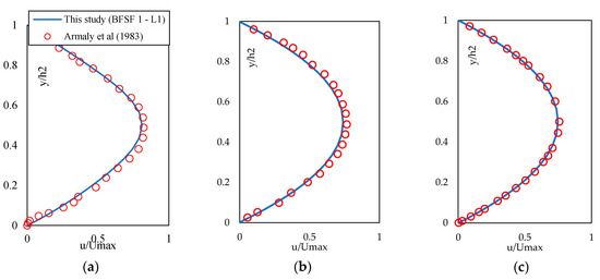
Figure 6. Dimensionless u-velocity profiles (u/U_max) at Re_h = 75. (a) x/h = 4.8, (b) x/h = 12.04, (c) x/h = 30.31 [3].

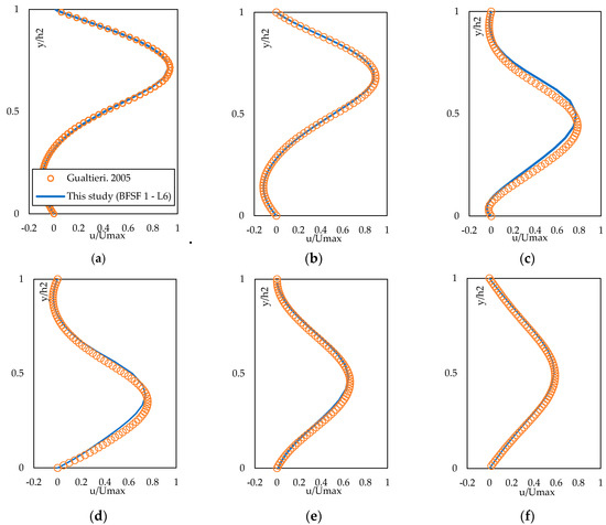
Figure 7. Dimensionless u-velocity profiles (u/U_max) at Re_h = 672. (a) x/h = 5, (b) x/h = 7.5, (c) x/h = 12, (d) x/h = 15, (e) x/h = 22.5, (f) x/h = 30 [23].

The locations were chosen at different locations, including recirculation zones at the upper and bottom walls. The u-velocity profiles showed that the flow separated at the step, resulting in recirculation regions downstream of the step, and then redeveloped into a fully developed parabolic velocity profile in the larger channel. This coincides with data reported in the literature [3]. The u-velocity distributions were compared quantitatively at different locations of the domain downstream of the step with the experimental data of Armaly et al. [3] and the numerical results of Gualtieri [23]. The results were consistent with the literature data and the average error between numerical and literature data for ranges of Reynolds numbers were lower than 8.1%.

3.1.3. Skin Friction Distribution

The boundary layer is associated with important characteristics such as the skin friction coefficient. The skin friction coefficient, C_f, is a dimensionless quantity derived from the averaged wall shear stress (τ_w) as

$${\mathrm{C}}_{\mathrm{f}}=\frac{{2\mathsf{\tau }}_{\mathrm{w}}}{{\mathsf{\rho }\mathrm{u}}^2}.$$

(12)

The distribution of the skin friction coefficient (C_f) at the bottom wall was calculated. The minimum peak of the skin friction coefficient (C_{f, min}) compared with the experimental data and numerical results of Tihon et al. [19] in Figure 8. For comparison, in Figure 8, the Reynolds numbers were modified by the Reynolds number of Tihon et al. [19].

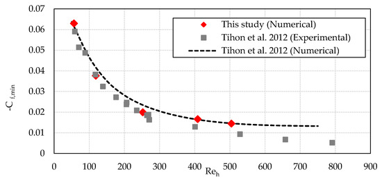
Figure 8. Dimensionless C_{f, min} vs. Re_h in laminar flow [19].

The minimum peak of the skin friction coefficient (C_{f, min}) was observed inside the primary recirculation zone. The average error between the numerical results of this study and the literature experimental and numerical results [19] was lower than 20% and 8.5%, respectively.

3.2. Turbulent Flow

3.2.1. Recirculation Zone and Reattachment Length

As in laminar flow, the flow separated at the sharp corner of the step and reattached downstream at the bottom wall. The reattachment lengths of the 2D BFSF in four turbulence models (standard k-ε, RNG k-ε, standard k-ω, and SST k-ω,) were compared with literature experimental data [1,3,54,55,56] and numerical results [1,30,57,58,59,60,61,62,63,64]. The data were plotted in Figure 9 as the normalized reattachment length by the step height against the Reynolds number (Re_h).

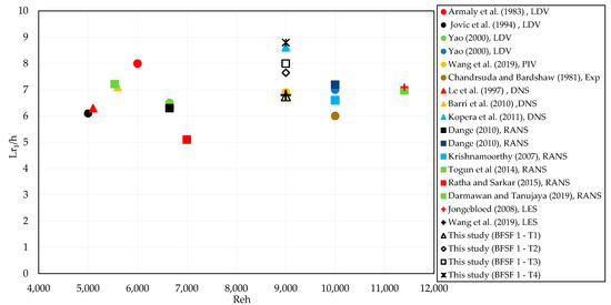
Figure 9. Dimensionless primary reattachment length (Lr₁/h) vs. Re_h in turbulent flow [1,3,30,54,55,56,57,58,59,60,61,62,63,64].

In the turbulent flow over the backward-facing step, the reattachment length is independent of the step-height Reynolds number- and is mostly between 5 and 8 times the step height. This is consistent with the present study. The present numerical results were compared with experimental data and numerical results [1] at Re_h = 9000 and ER = 2. Table 9 lists the value of the reattachment lengths in the BFSF.

Table 9. Reattachment length in past numerical and experimental works.

Case	Reh	ER	Lr1/h	Remarks *
This study (BFSF 1–T1)	9000	2	6.75	Num, 2D
This study (BFSF 1–T2)	9000	2	7.65	Num, 2D
This study (BFSF 1–T2)	9000	2	8	Num, 2D
This study (BFSF 1–T2)	9000	2	8.8	Num, 2D
Kopera et al. [30]	9000	2	8.62	Num, 3D
Araujo and Rezende [29]	9000	2	6.34	Num, 2D
Wang et al. [1]	9000	2	6.9	Exp, 3D
Wang et al. [1]	9000	2	6.7	Num, 2D

* Exp, experimental study; Num, numerical study; 2D, two-dimensional; 3D, three-dimensional.

The most accurate model in predicting Lr₁ was the standard k-ε, followed by RNG k-ε, standard k-ω, and SST k-ω. The average error between the standard k-ε model with the experimental and two-dimensional numerical results [1] was lower than 3% and 6%, respectively.

3.2.2. Vertical Profiles of the Streamwise Velocity

The distribution of the u-velocity of the 2D BFSF in different turbulence models was compared with previous studies [1,30] at different locations (Figure 10).

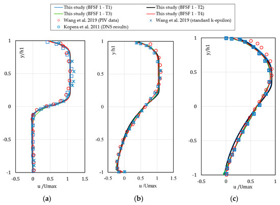
Figure 10. Dimensionless u-velocity (u/U_max) vertical profiles at (a) x/Lr₁ = 0.06, (b) x/Lr₁ = 0.46, (c) x/Lr₁ = 0.93, [1,30].

The first location (x/Lr₁ = 0.06) velocity was found near the step, consistent with the PIV data by Wang et al. [1]. The negative velocity in location x/Lr₁ = 0.46, represented the presence of inverse flow in the primary recirculation zone. In x/Lr₁ = 0.93, the standard k-ω, SST k-ω, and RNG k-ε models presented negative velocity because their Lr₁ was the largest among all models. The average error of velocity profiles between the present numerical results and literature experimental data [1] is shown in Table 10.

Table 10. Average errors (%) between numerical results of the velocity profiles with experimental data [1].

Turbulence Models	Standard k-ε	RNG k-ε	Standard k-ω	SST k-ω
Average error	<9.88%	<10.05%	<9.31%	<8.8%

The average error between the present two-dimensional numerical results and literature experimental data [1] was from 8.8% to 10.05%. The most accurate model in predicting velocity profiles was the SST k-ω, followed by the standard k-ω, standard k-ε, and RNG k-ε. The SST k-ω model was already recommended for cases with adverse pressure gradient and flow separation because it combines the advantages of the standard k-ω and standard k-ε models [29].

3.2.3. Skin Friction Distribution

The distribution of skin friction coefficient (C_f) at the bottom wall for different turbulence models were compared with literature data [8,15,30,65] in Figure 11.

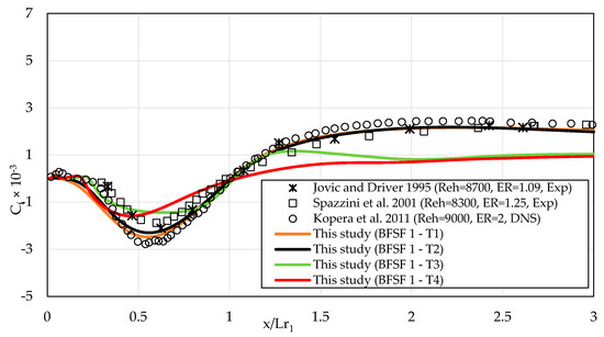
Figure 11. Longitudinal distribution of C_f at the bottom wall downstream of the step [15,30,65].

The results were compared with the available numerical result [30] at Re_h = 9000 and ER = 2. The distribution of skin friction in the standard k-ε and RNG k-ε turbulence models was consistent with that of the literature experimental data [15,65] and numerical results [30]. The average error was lower than 17.5%. The most accurate model in predicting skin friction coefficient was the standard k-ε, followed by RNG k-ε, standard k-ω, and SST k-ω. The standard k-ω, and SST k-ω were not good enough to capture the skin friction coefficient near the bottom wall.

As laminar flow, the C_f decreased and reached the minimum peak in the recirculation zone and gradually recovers to positive values after the reattachment point. A minimum peak of the skin friction coefficient was observed within the recirculating region. Tihon et al. [16] found that the minimum peak of skin friction inside of the recirculation zone was Reynolds number-dependent as

$${\mathrm{C}}_{\mathrm{f},\min }=-0{.38 \mathrm{Re}}_{\mathrm{h}}{}^{-0.57}.$$

(13)

The minimum peak of skin friction C_{f, min} obtained from the standard k-ɛ model was compared with the experimental data [15,16] and numerical results [26,37] (Figure 12). The present numerical results fit well with equation 13 and the literature data.

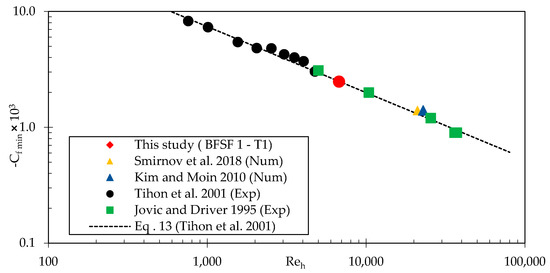
Figure 12. Dimensionless minimum peak of the skin friction coefficient (C_{f, min}) vs. (Re_h), [15,16,26,37].

3.2.4. Static Pressure Coefficient

One of the most important characteristics of the bottom wall is the pressure coefficient. The wall static pressure coefficient is defined as

$${\mathrm{C}}_{\mathrm{p}}=\frac{{\mathrm{P}-\mathrm{P}}_0}{0{.5\rho \mathrm{u}}^2},$$

(14)

where P is the wall static pressure in any location and P₀ is the reference wall static pressure measured at x = −4h, y = 1.5h (h is step height) upstream of the step as suggested by Kopera et al. [30].

The static pressure increased starting from the corner of the bottom wall. The distribution of pressure farther downstream of the step remained relatively stable in the flow recovery process. According to Kim et al. [39], to normalize the variations due to the different expansion ratios of BFSF, the normalized pressure coefficient (C*_p) was defined as

$${\mathrm{C}*}_{\mathrm{p}}=\frac{{\mathrm{C}}_{\mathrm{p}}{-\mathrm{C}}_{\mathrm{p}, \min }}{{\mathrm{C}}_{\mathrm{p}, \mathrm{Bc}}{-\mathrm{C}}_{\mathrm{p}, \min }},$$

(15)

where C_{p, min} is the minimum pressure coefficient and ${\mathrm{C}}_{\mathrm{p}, \mathrm{BC}}=\frac{2}{\mathrm{ER}}(1-\frac{1}{\mathrm{ER}}$) is the Borda–Carnot pressure coefficient [39]. The normalized pressure coefficients (C*_p) against the location scaled with the reattachment position, were compared in Figure 13.

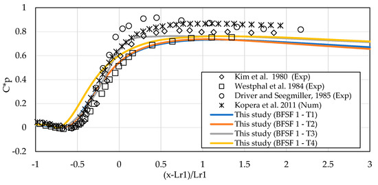
Figure 13. Longitudinal normalized pressure coefficient (C*_p) at the bottom wall downstream of the step [30,39,66,67].

The C*_p values computed by the different turbulence models at the bottom wall agreed with literature experimental data [39,66,67] and numerical results [30]. A sharp increase of pressure was observed in the reattachment zone (from x = 3h to x = 7h), consistent with the literature results [30,39,66,67]. The distribution of pressure farther downstream remained relatively stable in the flow recovery process. The most accurate model in predicting normalized pressure coefficients was the standard k-ε followed by standard k-ω, RNG k-ε, and SST k-ω with an average error lower than 20.5%.

4. Discussion

Flow over a backward-facing step could be found in many engineering applications in which there is a recirculation zone or sudden change in pressure. In Part 1 of this two-part paper, laminar and turbulent backward-facing step flow (BFSF) were studied. To validate the results herein, several study cases were conducted, and the numerical results were compared with literature numerical and experimental data. The following conclusions can be drawn.

• Laminar backward-facing step flow was investigated for a wide range of Reynolds numbers 75 ≤ Re_h ≤ 755 and the simulated reattachment lengths, velocity profiles, and skin frictions were compared with the available literature data. The average error between the present numerical results and literature numerical and experimental data for reattachment lengths and velocity profiles was lower than 8.1% and 18%, respectively. In addition, the average error in predicting the skin friction coefficient was lower than 20%.
• In turbulent flow, the simulated reattachment lengths, velocity profiles, skin friction coefficients, and pressure coefficient from several RANS models, standard k-ε, RNG k-ε, standard k-ω, SST k-ω, were compared with the available literature data. The most accurate model for predicting reattachment lengths, skin friction coefficient, and pressure coefficients was the standard k-ε model with an average error lower than 6, 17.5, and 20.5%, respectively.

5. Conclusions

In the present study, two geometries were comparatively considered, namely the classical BFSF (BFSF 1) and a BFSF with a cylinder placed downstream of the step (BFSF 2), in both laminar and turbulent flow to investigate how the cylinder modifies the classical two-dimensional BFSF structure by using the open-source code OpenFOAM. In Part 1, the results of the numerical study were validated by available literature data. First, the numerical results in laminar flow were found to be in good agreement with the literature experimental and numerical results. Secondly, the RANS model can predict the mean 2D flow structures of BFSF well. In turbulent flow, four turbulence models (standard k-ε, RNG k-ε, standard k-ω, and SST k-ω) were comparatively applied. Considering the accuracy and the calculation time of the models, only the standard k-ɛ model was used for the study of the effect of a cylinder placed downstream of the step. In Part 2, the effect on the 2D flow structure of a cylinder placed at different horizontal and vertical locations downstream of the step was investigated for both laminar and turbulent flow.

References

- Wang, F.-F.; Wu, S.-Q.; Zhu, S.-L. Numerical simulation of flow separation over a backward-facing step with high Reynolds number. Water Sci. Eng. 2019, 12, 145–154. [Google Scholar] [CrossRef]
- Abbott, D.E.; Kline, S.J. Experimental Investigation of Subsonic Turbulent Flow Over Single and Double Backward Facing Steps. J. Basic Eng. 1962, 84, 317–325. [Google Scholar] [CrossRef]
- Armaly, B.F.; Durst, F.; Pereira, J.C.F.; Schönung, B. Experimental and theoretical investigation of backward-facing step flow. J. Fluid Mech. 1983, 127, 473–496. [Google Scholar] [CrossRef]
- Kuehn, D.M. Effects of Adverse Pressure Gradient on the Incompressible Reattaching Flow over a Rearward-Facing Step. AIAA J. 1980, 18, 343–344. [Google Scholar] [CrossRef]
- Ötügen, M. Expansion ratio effects on the separated shear layer and reattachment downstream of a backward-facing step. Exp. Fluids 1991, 10, 273–280. [Google Scholar] [CrossRef]
- Durst, F.; Tropea, C. Flows over two-dimensional backward—Facing steps. In Structure of Complex Turbulent Shear Flow; Springer: Berlin/Heidelberg, Germany, 1983; pp. 41–52. [Google Scholar]
- Adams, E.W.; Johnston, J.P. Effects of the separating shear layer on the reattachment flow structure Part 1: Pressure and turbulence quantities. Exp. Fluids 1988, 6, 400–408. [Google Scholar] [CrossRef]
- Adams, E.W.; Johnston, J.P. Effects of the separating shear layer on the reattachment flow structure part 2: Reattachment length and wall shear stress. Exp. Fluids 1988, 6, 493–499. [Google Scholar] [CrossRef]
- Kim, J.J. Investigation of Separation and Reattachment of a Turbulent Shear Layer: Flow over a Backward-Facing Step; Stanford University: Stanford, CA, USA, 1978. [Google Scholar]
- Biswas, G.; Breuer, M.; Durst, F. Backward-facing step flows for various expansion ratios at low and moderate Reynolds numbers. J. Fluids Eng. 2004, 126, 362–374. [Google Scholar] [CrossRef]
- Singh, A.; Paul, A.; Ranjan, P. Investigation of reattachment length for a turbulent flow over a backward facing step for different step angle. Int. J. Eng. Sci. Technol. 2011, 3. [Google Scholar] [CrossRef]
- Moss, W.; Baker, S.; Bradbury, L. Measurements of mean velocity and Reynolds stresses in some regions of recirculating flow. In Turbulent Shear Flows I; Springer: Berlin/Heidelberg, Germany, 1979; pp. 198–207. [Google Scholar]
- Heenan, A.; Morrison, J. Passive control of pressure fluctuations generated by separated flow. AIAA J. 1998, 36, 1014–1022. [Google Scholar] [CrossRef]
- Lee, T.; Mateescu, D. Experimental and numerical investigation of 2-d backward-facing step flow. J. Fluids Struct. 1998, 12, 703–716. [Google Scholar] [CrossRef]
- Jovic, S.; Driver, D. Reynolds number effect on the skin friction in separated flows behind a backward-facing step. Exp. Fluids 1995, 18, 464–467. [Google Scholar] [CrossRef]
- Tihon, J.; Legrand, J.; Legentilhomme, P. Near-wall investigation of backward-facing step flows. Exp. Fluids 2001, 31, 484–493. [Google Scholar] [CrossRef]
- Furuichi, N.; Hachiga, T.; Kumada, M. An experimental investigation of a large-scale structure of a two-dimensional backward-facing step by using advanced multi-point LDV. Exp. Fluids 2004, 36, 274–281. [Google Scholar] [CrossRef]
- Bouda, N.N.; Schiestel, R.; Amielh, M.; Rey, C.; Benabid, T. Experimental approach and numerical prediction of a turbulent wall jet over a backward facing step. Int. J. Heat Fluid Flow 2008, 29, 927–944. [Google Scholar] [CrossRef]
- Tihon, J.; Pěnkavová, V.; Havlica, J.; Šimčík, M. The transitional backward-facing step flow in a water channel with variable expansion geometry. Exp. Therm. Fluid Sci. 2012, 40, 112–125. [Google Scholar] [CrossRef]
- Gautier, N.; Aider, J.-L. Feed-forward control of a perturbed backward-facing step flow. J. Fluid Mech. 2014, 759, 181–196. [Google Scholar]
- Toumey, J.; Zhang, P.; Zhao, X.; Colborn, J.; O’Connor, J.A. Assessing the wall effects of backwards-facing step flow in tightly-coupled experiments and simulations. In Proceedings of the AIAA SCITECH 2022 Forum, San Diego, CA, USA, 29 December 2022; p. 0822. [Google Scholar] [CrossRef]
- Chen, L.; Asai, K.; Nonomura, T.; Xi, G.; Liu, T. A review of Backward-Facing Step (BFS) flow mechanisms, heat transfer and control. Therm. Sci. Eng. Prog. 2018, 6, 194–216. [Google Scholar] [CrossRef]
- Gualtieri, C. Numerical simulations of laminar backward-facing step flow with FemLab 3.1. In Proceedings of the Fluids Engineering Division Summer Meeting, Houston, TX, USA, 13 October 2005; pp. 657–662. [Google Scholar]
- Yang, X.-D.; Ma, H.-Y.; Huang, Y.-N. Prediction of homogeneous shear flow and a backward-facing step flow with some linear and non-linear K–ε turbulence models. Commun. Nonlinear Sci. Numer. Simul. 2005, 10, 315–328. [Google Scholar] [CrossRef]
- Erturk, E. Numerical solutions of 2-D steady incompressible flow over a backward-facing step, Part I: High Reynolds number solutions. Comput. Fluids 2008, 37, 633–655. [Google Scholar] [CrossRef]
- Kim, D.; Moin, P. Direct numerical study of air layer drag reduction phenomenon over a backward-facing step. Cent. Turbul. Res. Annu. Res. Briefs 2010, 351–363. [Google Scholar]
- Jehad, D.; Hashim, G.; Zarzoor, A.; Azwadi, C.N. Numerical study of turbulent flow over backward-facing step with different turbulence models. J. Adv. Res. Des. 2015, 4, 20–27. [Google Scholar]
- Al-Jelawy, H.; Kaczmarczyk, S.; AlKhafaji, D.; Mirhadizadeh, S.; Lewis, R.; Cross, M. A computational investigation of a turbulent flow over a backward facing step with OpenFOAM. In Proceedings of the 2016 9th International Conference on Developments in eSystems Engineering (DeSE), Liverpool, UK, 31 August–2 September 2016; pp. 301–307. [Google Scholar]
- Araujo, P.P.; Rezende, A.L.T. Comparison of turbulence models in the flow over a backward-facing step. Int. J. Eng. Res. Sci. 2017, 3, 88–93. [Google Scholar] [CrossRef]
- Kopera, M.A.; Kerr, R.M.; Blackburn, H.; Barkley, D. Direct Numerical Simulation of Turbulent Flow over a Backward-Facing Step. Doctoral Dissertation, University of Warwick, 2011. Available online: http://go.warwick.ac.uk/wrap/47811 (accessed on 28 December 2022).
- Singh, A.; Aravind, S.; Srinadhi, K.; Kannan, B. Assessment of Turbulence Models on a Backward Facing Step Flow Using OpenFOAM®. Mater. Sci. Eng. 2020, 1274, 042060. [Google Scholar] [CrossRef]
- DeBonis, J.R. A Large-Eddy Simulation Of Turbulent Flow Over A Backward Facing Step. In Proceedings of the AIAA SCITECH 2022 Forum, San Diego, CA, USA, 29 December 2022; p. 0337. [Google Scholar]
- Abdollahpour, M.; Gualtieri, P.; Gualtieri, C. Influence of a Rigid Cylinder on Flow Structure over a Backward-Facing Step. In Proceedings of the 39th IAHR World Congress, 19–24 June 2022; p. 24. [Google Scholar]
- Gaur, N.; Lingeshwar, R.; Kannan, B. Computational analysis of backward facing step flow using OpenFOAM®. AIP Conf. Proc. 2022, 2516, 030005. [Google Scholar]
- Abdollahpour, M.; Gualtieri, P.; Gualtieri, C. Numerical simulation of turbulent flow past a cylinder placed downstream of a step. Environ. Sci. Proc. 2022, 21, 58. [Google Scholar]
- Shu, C.; Peng, Y.; Zhou, C.F.; Chew, Y.T. Application of Taylor series expansion and Least-squares-based lattice Boltzmann method to simulate turbulent flows. J. Turbul. 2006, 7, N38. [Google Scholar] [CrossRef]
- Smirnov, E.M.; Smirnovsky, A.A.; Schur, N.A.; Zaitsev, D.K.; Smirnov, P.E. Comparison of RANS and IDDES solutions for turbulent flow and heat transfer past a backward-facing step. Heat Mass Transf. 2018, 54, 2231–2241. [Google Scholar] [CrossRef]
- Anwar-ul-Haque, F.A.; Yamada, S.; Chaudhry, S.R. Assessment of turbulence models for turbulent flow over backward facing step. In Proceedings of the Proceedings of the World Congress on Engineering, London, UK, 2–4 July 2007; pp. 2–7.
- Kim, J.; Kline, S.J.; Johnston, J.P. Investigation of a Reattaching Turbulent Shear Layer: Flow Over a Backward-Facing Step. J. Fluids Eng. 1980, 102, 302–308. [Google Scholar] [CrossRef]
- Cruz, D.O.d.A.; Batista, F.; Bortolus, M. A law of the wall formulation for recirculating flows. J. Braz. Soc. Mech. Sci. 2000, 22, 43–51. [Google Scholar] [CrossRef]
- Wang, Y.; Yang, Y.; Ma, G.; Zhou, Y.-m. Numerical analysis of flow noises in the square cavity vortex based on computational fluid dynamics. J. Vibroengineering 2016, 18, 2656–2666. [Google Scholar] [CrossRef]
- Roache, P.J. Quantification of uncertainty in computational fluid dynamics. Annu. Rev. Fluid Mech. 1997, 29, 123–160. [Google Scholar] [CrossRef]
- Roache, P.J. Perspective: Validation—What does it mean? ASME 2009, 131, 34503. [Google Scholar] [CrossRef]
- Blocken, B.; Gualtieri, C. Ten iterative steps for model development and evaluation applied to Computational Fluid Dynamics for Environmental Fluid Mechanics. Environ. Model. Softw. 2012, 33, 1–22. [Google Scholar] [CrossRef]
- Biswas, R.; Strawn, R.C. Tetrahedral and hexahedral mesh adaptation for CFD problems. Appl. Numer. Math. 1998, 26, 135–151. [Google Scholar] [CrossRef]
- Keyes, D.; Ecer, A.; Satofuka, N.; Fox, P.; Periaux, J. Parallel Computational Fluid Dynamics’ 99: Towards Teraflops, Optimization and Novel Formulations; Elsevier: Amsterdam, The Netherlands, 2000. [Google Scholar]
- Nguyen, T.H.T.; Ahn, J.; Park, S.W. Numerical and physical investigation of the performance of turbulence modeling schemes around a scour hole downstream of a fixed bed protection. Water 2018, 10, 103. [Google Scholar] [CrossRef]
- Viti, N.; Valero, D.; Gualtieri, C. Numerical simulation of hydraulic jumps. Part 2: Recent results and future outlook. Water 2018, 11, 28. [Google Scholar] [CrossRef]
- Launder, B.E.; Spalding, D.B. Lectures in mathematical models of turbulence. AGRIS 1972. [Google Scholar]
- Yakhot, V.; Orszag, S.A. Renormalization group analysis of turbulence. I. Basic theory. J. Sci. Comput. 1986, 1, 3–51. [Google Scholar] [CrossRef]
- Wilcox, D.C. Turbulence Modeling for CFD; DCW Industries: La Canada, CA, USA, 1998; Volume 2. [Google Scholar]
- Cherdron, W.; Durst, F.; Whitelaw, J.H. Asymmetric flows and instabilities in symmetric ducts with sudden expansions. J. Fluid Mech. 1978, 84, 13–31. [Google Scholar] [CrossRef]
- Sparrow, E.; Kalejs, J. Local convective transfer coefficients in a channel downstream of a partially constricted inlet. Int. J. Heat Mass Transf. 1977, 20, 1241–1249. [Google Scholar] [CrossRef]
- Yao, S. Two Dimensional Backward Facing Single Step Flow Preceding an Automotive Air-Filter; Oklahoma State University: Stillwater, OK, USA, 2000. [Google Scholar]
- Jovic, S.; Driver, D.M. Backward-Facing Step Measurements at Low Reynolds Number, Re (sub h)= 5000; No. NASA-TM-108807; NASA: Washington, DC, USA, 1994. [Google Scholar]
- Chandrsuda, C.; Bradshaw, P. Turbulence structure of a reattaching mixing layer. J. Fluid Mech. 1981, 110, 171–194. [Google Scholar] [CrossRef]
- Barri, M.; El Khoury, G.K.; Andersson, H.I.; Pettersen, B. DNS of backward-facing step flow with fully turbulent inflow. Int. J. Numer. Methods Fluids 2010, 64, 777–792. [Google Scholar] [CrossRef]
- Dange, A. Modeling of Turbulent Particulate Flow in the Recirculation Zone Downstream of a Backward Facing Step Preceding a Porous Medium; Oklahoma State University: Stillwater, OK, USA, 2010. [Google Scholar]
- Togun, H.; Safaei, M.R.; Sadri, R.; Kazi, S.N.; Badarudin, A.; Hooman, K.; Sadeghinezhad, E. Numerical simulation of laminar to turbulent nanofluid flow and heat transfer over a backward-facing step. Appl. Math. Comput. 2014, 239, 153–170. [Google Scholar] [CrossRef]
- Ratha, D.; Sarkar, A. Analysis of flow over backward facing step with transition. Front. Struct. Civil Eng. 2015, 9, 71–81. [Google Scholar] [CrossRef]
- Krishnamoorthy, C. Numerical Analysis of Backward-Facing Step Flow Preceeding a Porous Medium Using FLUENT; Oklahoma State University: Stillwater, OK, USA, 2007. [Google Scholar]
- Jongebloed, L. Numerical Study Using FLUENT of the Separation and Reattachment Points for Backwards-Facing Step Flow. Master’s Thesis, Mechanical Engineering, Rensselaer Polytechnic Institute, Troy, NY, USA, 2008. [Google Scholar]
- Darmawan, S.; Tanujaya, H. CFD Investigation of Flow Over a Backward-facing Step using an RNG k-? Turbulence Model. Int. J. Technol. 2019, 10, 280. [Google Scholar] [CrossRef]
- LE, H.; Moin, P.; Kim, J. Direct numerical simulation of turbulent flow over a backward-facing step. J. Fluid Mech. 1997, 330, 349–374. [Google Scholar] [CrossRef]
- Spazzini, P.G.; Iuso, G.; Onorato, M.; Zurlo, N.; Di Cicca, G.M. Unsteady behavior of back-facing step flow. Exp. Fluids 2001, 30, 551–561. [Google Scholar] [CrossRef]
- Driver, D.M.; Seegmiller, H.L. Features of a reattaching turbulent shear layer in divergent channelflow. AIAA J. 1985, 23, 163–171. [Google Scholar] [CrossRef]
- Westphal, R.V.; Johnston, J.; Eaton, J. Experimental Study of Flow Reattachment in a Single-Sided Sudden Expansion; NASA: Washington, DC, USA, 1984.
Disclaimer/Publisher’s Note: The statements, opinions and data contained in all publications are solely those of the individual author(s) and contributor(s) and not of MDPI and/or the editor(s). MDPI and/or the editor(s) disclaim responsibility for any injury to people or property resulting from any ideas, methods, instructions or products referred to in the content. |
© 2023 by the authors. Licensee MDPI, Basel, Switzerland. This article is an open access article distributed under the terms and conditions of the Creative Commons Attribution (CC BY) license (https://creativecommons.org/licenses/by/4.0/).