Compressible and Viscous Effects in Transonic Planar Flow around a Circular Cylinder—A Numerical Analysis Based on a Commercially Available CFD Tool

Abstract

Transonic planar flows around a circular cylinder are investigated numerically for laminar and turbulent flow conditions with Reynolds numbers of $50\le R{e}_D\le 300$ and $8890\le R{e}_D\le$ 80,000 and free stream Mach numbers in the range of $0.2\le M{a}_{\infty }\le 2$. A commercially available CFD tool is used and validated for this purpose. The results show that the flow phenomena occurring can be grouped into eight regimes. Compared to the incompressible flow regimes, several new phenomena can be found. In contrast, at higher $M{a}_{\infty }$ of $0.6\le M{a}_{\infty }\le 0.8$ vortices in the wake of the cylinder are suppressed for $R{e}_D=50$. In some cases, $M{a}_{\infty }=0.8$ and $R{e}_D\ge 300$, $\lambda$-shocks are formed in the near cylinder wake. For supersonic $M{a}_{\infty }$, two different phenomena are observed. Beside the well-known oblique and detached shocks, for $50\le R{e}_D\le 300$ a wake with instabilities is formed downstream of the cylinder. Furthermore, the temporal mean drag coefficient ${\overline{C}}_{\mathrm{D}}$, the Strouhal number $Str$, as well as the critical Mach number $M{a}_{\mathrm{crit}}$ are calculated from the simulation results and are interpreted.

1. Introduction

The flow around a circular cylinder is encountered in many engineering applications as well as in nature and in fundamental research. Some examples are the air flow around a cooling tower, as well as missiles and aircrafts in the transonic regime. In transonic flows and fluid dynamical situations in general, a variety of typical phenomena, such as shock waves, vortices, boundary layers, flow separation and shear layers, arise. Studying the interaction of those phenomena is of large interest in fluid–structure interactions, because resonance frequencies can be excited by flow instabilities. The question arises as to what frequency is triggered by the flow around a cylinder, which could provoke an oscillation. In dimensionless terms, this means that the Strouhal number $Str$ becomes a function not only of the Reynolds number $R{e}_D$, but also of the Mach number $M{a}_{\infty }$. In practical situations embedded in a larger project context, where questions like the mentioned one arise, one often does not have the time nor the resources to develop one’s own numerical tool for simulation and calculation. Rather, one has to refer to methods and tools available on the market; that is why the investigation described here is based on a commercially available CFD tool. It is clear, though, that such a tool has to be checked appropriately before the corresponding findings can be used.

There are various studies describing the flow phenomena occurring in incompressible flow. For small Reynolds numbers in the range of $80\le R{e}_D\le 300$, a Kármán vortex street is formed in the wake of the cylinder described by Schlichting and Gersten [1]. Although the flow around a circular cylinder has received a lot of attention in recent decades, very few experimental and numerical studies are available about the compressible and in particular transonic flow around a circular cylinder. One of the reasons might be the difficulties in performing experiments of simple flow situations such as the planar flow around a circular cylinder. However, planar aerodynamical investigations are also of interest, as they allow one, for example, to estimate in a simplified manner the force on a body in a surrounding transonic flow. The most important experimental studies and their findings are summarised below.

Macha [2] performed wind tunnel tests in order to determine the drag coefficient ${\overline{C}}_{\mathrm{D}}$ for a Reynolds number range of $5\times {10}^4\le R{e}_D\le 8.7\times {10}^6$ and a Mach number range of $0.2\le M{a}_{\infty }\le 1.4$. One of the most important findings is the reduction in ${\overline{C}}_{\mathrm{D}}$ from $M{a}_{\infty }=0.7$ to $0.8$, caused by the formation of shock waves. In addition, Murthy and Rose [3] performed a series of wind tunnel tests with $0.25\le M{a}_{\infty }\le 1.2$ and $3\times {10}^4\le R{e}_D\le 5\times {10}^5$. The increase in ${\overline{C}}_{\mathrm{D}}$, as $M{a}_{\infty }$ reaches sonic conditions and agrees with the findings of Macha [2]. Furthermore, it was found that the detectable vortex shedding ceases at $M{a}_{\infty }\ge 0.9$. The ranges $0.4\le M{a}_{\infty }\le 0.85$ and $1.7\times {10}^5\le R{e}_D\le 3.4\times {10}^5$ were investigated by Rodriguez [4] using a wind tunnel. It was found that the coupling between the near wake and the vortex street increases with increasing $M{a}_{\infty }$. As soon as local regions of the flow reach sonic conditions and $\lambda$ shocks occur, the coupling between the vortex street and the near wake is cut off. The upstream flow field is now independent of the vortex street. In addition, the Strouhal number $Str$ is approximately 0.2, except for a rise when the quasi-steady regime is reached. In addition, the drag and lift coefficients, $C_{\mathrm{D}}$ and $C_{\mathrm{L}}$, were calculated from the pressure measurements. Ackerman et al. [5] experimentally investigated time-resolved pressure distributions at $0.1\le M{a}_{\infty }\le 0.9$ and $R{e}_D=6.83\times {10}^5$. From these measurements, the surface pressure fluctuations, ${\overline{C}}_{\mathrm{D}}$, $Str$ and the occurring flow regimes were evaluated. For $M{a}_{\infty }=0.4$, local regions of flow around the cylinder reach sonic conditions, but only on one side of the cylinder at a time. The flow enters the intermittent shock wave regime. As $M{a}_{\infty }$ increases beyond 0.4, ${\overline{C}}_{\mathrm{D}}$ increases. The region downstream of the cylinder, in which the vortices are formed, shortens. Beyond around $M{a}_{\infty }=0.65$, the flow enters the permanent shock wave regime and ${\overline{C}}_{\mathrm{D}}$ decreases. Once the flow enters the wake shock wave regime below $M{a}_{\infty }=0.8$, the vortex formation region becomes elongated. A normal shock grows at the point of vortex roll up and ${\overline{C}}_{\mathrm{D}}$ increases. Nagata et al. [6] used a low-density wind tunnel with time-resolved Schlieren visualisations, pressure and force measurements, in order to characterise the flow for $1000\le R{e}_D\le 5000$ and $0.1\le M{a}_{\infty }\le 0.5$. The trend of the $M{a}_{\infty }$ effect on the flow field, $Str$ and the maximum width of the recirculation change at approximately $R{e}_D=3000$. $Str$ increases as $R{e}_D$ increases and the increment becomes larger as $M{a}_{\infty }$ increases. For $M{a}_{\infty }<0.3$, $Str$ is independent of $M{a}_{\infty }$. For $R{e}_D\le 3000$ and $R{e}_D\ge 4000$ at $M{a}_{\infty }>0.3$, $Str$ decreases and increases, respectively. Furthermore, it is observed that ${\overline{C}}_{\mathrm{D}}$ increases as $M{a}_{\infty }$ or $R{e}_D$ increase. Gowen and Perkins [7] measured the pressure distribution around a circular cylinder in subsonic and supersonic flows and calculated ${\overline{C}}_{\mathrm{D}}$ for $5\times {10}^4\le R{e}_D\le {10}^6$ and $0.3\le M{a}_{\infty }\le 2.9$. It is shown that ${\overline{C}}_{\mathrm{D}}$ is not influenced by $R{e}_D$ under the supersonic conditions investigated.

In addition to the experimental investigations, numerical simulations of the compressible flow around a circular cylinder have been increasingly carried out over the last few decades. Some examples of numerical investigations are described below. Botta [8] integrated the Euler equations numerically to investigate the inviscid flow for $0.38\le M{a}_{\infty }\le 0.98$, that means for a Reynolds number $R{e}_D\to \infty$. The time-dependent $C_{\mathrm{D}}$ and $C_{\mathrm{L}}$ are evaluated in order to determine $Str$. Furthermore, the distributions of the vorticity, the entropy deviation, pressure coefficient, as well as the velocity fields are provided. Two transitions over the investigated $M{a}_{\infty }$ range were observed, the transition to a chaotic turbulent regime and from this to a quasi-steady flow. In the range $0.5\le M{a}_{\infty }\le 0.6$, the solution shows a periodic behaviour. Bobenrieth Miserda and Leal [9] performed numerical Detached Eddy Simulations of the unsteady transonic flow at $M{a}_{\infty }=0.8$ and $R{e}_D=$ 500,000, where several complex viscous shock interactions were observed. The frequency of $C_{\mathrm{L}}$ corresponds to the vortex-shedding frequency, whereas the frequency of the $C_{\mathrm{D}}$ characterises the viscous shock interaction. In addition, Xu et al. [10] performed Detached Eddy Simulations for $R{e}_D=2\times {10}^5$ and various Mach numbers $0.85\le M{a}_{\infty }\le 0.98$. Two flow states are found, an unsteady one for $M{a}_{\infty }<0.9$ and a quasi-steady flow state for $M{a}_{\infty }>0.9$. The unsteady flow state is characterised by the interaction of moving shock waves, the turbulent boundary layer on the cylinder wall and the vortex shedding in the cylinders near the wake. In the quasi-steady flow state, strong oblique shock waves are formed and the vortex shedding is suppressed. Furthermore, the local supersonic zone, the separation angle and ${\overline{C}}_{\mathrm{D}}$ are evaluated and analysed. Hong et al. [11] studied $0.1\le M{a}_{\infty }\le 0.95$ and $R{e}_D=2\times {10}^5$ using constrained Large Eddy Simulations. The effects of $M{a}_{\infty }$ on the flow patterns and state variables such as the pressure, the skin friction, $C_{\mathrm{D}}$ and the cylinder surface temperature are studied. Non-monotonic behaviour of the pressure and skin friction distributions are observed with increasing $M{a}_{\infty }$. The minimum mean separation angle occurs at $0.3\le M{a}_{\infty }\le 0.5$. Canuto and Taira [12] performed Direct Numerical Simulations of $20\le R{e}_D\le 100$ and $0\le M{a}_{\infty }\le 0.5$. The wake is characterised using different lengths and ${\overline{C}}_{\mathrm{D}}$, and $Str$ and some examples of the pressure distribution are provided. Furthermore, a stability analysis is performed. It is shown that ${\overline{C}}_{\mathrm{D}}$ increases and $Str$ decreases with increasing $M{a}_{\infty }$ for constant $R{e}_D$. Xia et al. [13] performed constrained Large Eddy Simulations for $R{e}_D=4\times {10}^4$ and $R{e}_D={10}^6$ and various Mach numbers of $0.5\le M{a}_{\infty }\le 0.95$. The separation angle, ${\overline{C}}_{\mathrm{D}}$, the pressure distribution and the skin friction coefficient were evaluated and analysed. Furthermore, the density gradient $\left|\nabla \rho \right|$ was used to identify four different flow regimes. Shirani [14] simulated $0.1\le M{a}_{\infty }\le 0.9$ and ${10}^3\le R{e}_D\le 8.4\times {10}^6$ solving the two-dimensional time averaged Navier–Stokes equations numerically. The behaviour of the time averages of $C_{\mathrm{D}}$ and $C_{\mathrm{L}}$ and their fluctuation frequencies were evaluated. Matar et al. [15] investigated the real gas flow around a circular cylinder at high Reynolds numbers $R{e}_D$ and Mach numbers $M{a}_{\infty }$ between 0.7 and 0.9 using wall-resolved implicit Large Eddy Simulations (iLESs). For experimental validation at $M{a}_{\infty }=0.7$, Background Oriented Schlieren (BOS) visualisations are used. The flow phenomena of a Kármán vortex street, acoustic waves and compression waves are observed. In addition, the Strouhal number $Str$, the wall pressure and the mean pressure drag coefficients are provided and are compared with literature and URANS simulation results. In addition, Linn and Awruch [16] performed Large Eddy Simulations (LESs) of the two- and three-dimensional flow around a circular cylinder at $R{e}_D=$ 500,000 and $M{a}_{\infty }=0.8$ using various tetrahedron-adapted meshes. The density gradient $|\nabla \rho |$, the streamlines and Q-criterion isosurfaces are used to visualise the flow behaviour. Moreover, the drag and the lift coefficients $C_{\mathrm{D}}$ and $C_{\mathrm{L}}$, the Strouhal number $St{r}_{\mathrm{L}}$, the mean surface pressure coefficient and the angle of the boundary layer separation point are provided.

The present study describes the transonic planar flow around a circular cylinder at conditions $M{a}_{\infty }$ and $R{e}_D$ where only a few investigations have been carried out (Figure 1). The investigation of the planar situation enables one to analyse the phenomena uncoupled from the influence of potential three-dimensional effects. This investigation gives an overview of the flow phenomena occurring in a wide range of Mach numbers of $M{a}_{\infty }=0.2$ to 2 and Reynolds numbers of $R{e}_D=50$ to 80,000. Within the first few chapters, the fundamentals and the numerical implementation are briefly introduced. The simulations of the compressible flow around a circular cylinder are verified by applying the code used to the flow in a Laval nozzle. For validation, the results obtained for the flow around a cylinder are compared to the results from other authors. Different regimes with phenomena such as shock waves, sound waves, flow separation, vortex shedding, shear layers and tangential discontinuities are identified and some of them are analysed in more detail. To capture the different flow phenomena, different regions of interest are used for the numerical procedure. This investigation focuses on the behaviour in the wake of the cylinder. In addition, the critical Mach number $M{a}_{\mathrm{crit}}$ is evaluated and the averaged drag coefficient ${\overline{C}}_{\mathrm{D}}$ and the Strouhal number $Str$ are provided. Finally, polar diagrams are presented, that means the time-resolved drag and lift coefficients, $C_{\mathrm{D}}$ and $C_{\mathrm{L}}$, are plotted as a function of time in a $C_{\mathrm{D}}$-$C_{\mathrm{L}}$-diagram, to analyse their phase shift and their frequency ratio.

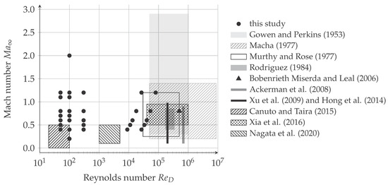
Figure 1. Conditions investigated in previous studies and in this study [2,3,4,5,6,7,9,10,11,12,13].

2. Fundamentals

Within this chapter, the most important fundamentals such as the governing equations solved in CFD and the dimensionless numbers used within this study are introduced.

2.1. Governing Equations

The three transport equations of mass, momentum and energy are called the Navier–Stokes equations, where only momentum and energy can be transported via conduction in all directions x, y and z. The general transport equation is shown in Equation (1) where $\phi$ is the transported property. In Table 1, the transport property $\phi$, the diffusion coefficient ${\mathsf{\Gamma }}_{\phi }$ and the source, loss and production term $S_{\phi }$ are specialised for the mass, momentum and energy transport equations.

$$\frac{\partial \phi }{\partial t}=-\nabla ·\left(\phi \overrightarrow{u}\right)+\nabla ·\left({\mathsf{\Gamma }}_{\phi }\nabla \phi \right)+S_{\phi }$$

(1)

The terms of Equation (1) can be described in words as follows.

Table 1. Specialisation for mass, momentum and energy for the Navier–Stokes equations.

	Transport Property $\mathit{\phi }$	Diffusion Coefficient ${\mathbf{\Gamma }}_{\mathit{\phi }}$ in m2 s−1	Source, Loss and Production ${\mathit{S}}_{\mathit{\phi }}$
Mass	Density $\rho$ in $\mathrm{k}\mathrm{g}{\mathrm{m}}^{-3}$	0	0
Momentum	Specific momentum $\rho u_i$ in $\mathrm{N}\mathrm{s}{\mathrm{m}}^{-3}$	Kinematic viscosity $\nu$	$S_{\rho u_i}$ in $\mathrm{N}{\mathrm{m}}^{-3}$
Energy	Specific enthalpy h in $\mathrm{J}{\mathrm{m}}^{-3}$	Thermal diffusivity ${\alpha }_{\mathrm{th}}$	$S_h$ in $\mathrm{W}{\mathrm{m}}^{-3}$

• $\frac{\partial \phi }{\partial t}$: Accumulation of $\phi$ in the control volume.
• $\nabla ·\left(\phi \overrightarrow{u}\right)$: Convective flux of $\phi$ across the surfaces of the control volume.
• $\nabla ·\left({\mathsf{\Gamma }}_{\phi }\nabla \phi \right)$: Conductive flux of $\phi$ across the surfaces of the control volume.
• $S_{\phi }$: Production and/or loss of $\phi$ in the control volume + external supply of $\phi$ in the control volume.

The fluid air is assumed to behave as an ideal gas; thus, the corresponding equation follows

$$p=\rho RT$$

(2)

where R denotes the specific gas constant, expressed in J kg⁻¹ K ⁻¹ and T the absolute temperature. Turbulence effects are described by means of the Shear Stress Transport (SST) model; see Section 3.1.

2.2. Classification of the Flow Regimes

The fluid flow is classified by means of the Reynolds and the Mach numbers $R{e}_D$ and $M{a}_{\infty }$. The Reynolds number $R{e}_D$ defined in Equation (3) describes the ratio of inertial forces to viscous forces and is used to predict the flow regime of laminar, transitional or turbulent flow. It is defined using the free stream density ${\rho }_{\infty }$ of the fluid, the free stream velocity $u_{\infty }$, the cylinder diameter D and the free stream dynamic viscosity ${\mu }_{\infty }$.

$$R{e}_D=\frac{{\rho }_{\infty }·u_{\infty }·D}{{\mu }_{\infty }}$$

(3)

For the Reynolds numbers above a critical Reynolds number $R{e}_{\mathrm{crit}}$, which depends on the flow situation (flow over a flat plate, pipe flow, etc.), the flow becomes turbulent, which means it behaves in a chaotic way and underlies random fluctuations. Nevertheless, it has to be said that $R{e}_{\mathrm{crit}}$ is only a guiding value; there is no abrupt transition from laminar to turbulent at a certain Reynolds number.

The free stream Mach number $M{a}_{\infty }$ is the ratio between the free stream velocity $u_{\infty }$ and the speed of sound $a_{\infty }$ in the far field.

$$M{a}_{\infty }=\frac{u_{\infty }}{a_{\infty }}$$

(4)

According to the local Mach number $Ma$, the flow is called subsonic if $Ma<1$, supersonic if $Ma>1$ and hypersonic if $Ma>5$. Transonic flows have regions of both types, subsonic and supersonic.

2.3. Further Dimensionless Numbers

The behaviour of the fluid flow can then further be characterised by additional dimensionless numbers, which are described in this chapter.

The Strouhal number $Str$ in Equation (5) describes periodically oscillating flow phenomena using the frequency of the particular oscillation f, the cylinder diameter D and the free stream velocity $u_{\infty }$.

$$Str=\frac{f·D}{u_{\infty }}$$

(5)

The drag and the lift coefficients $C_{\mathrm{D}}$ and $C_{\mathrm{L}}$, respectively, are defined in Equations (6) and (7) as the ratio of the particular component of the force acting on the cylinder, drag or lift force, $F_{\mathrm{D}}$ or $F_{\mathrm{L}}$, and the product of the dynamic pressure $\frac{{\rho }_{\infty }}{2}·u_{\infty }^2$ and the cylinder’s front face A.

$$C_{\mathrm{D}}=\frac{F_{\mathrm{D}}}{\frac{{\rho }_{\infty }}{2}·u_{\infty }^2·A}$$

(6)

$$C_{\mathrm{L}}=\frac{F_{\mathrm{L}}}{\frac{{\rho }_{\infty }}{2}·u_{\infty }^2·A}$$

(7)

3. Numerical Simulation

Simulations in the laminar and turbulent regimes have been performed. Figure 2 shows $M{a}_{\infty }$ and $R{e}_D$ of those simulations. Therefore, the simulations are carried out in groups with constant Reynolds number $R{e}_D$ or constant cylinder diameter D. The $R{e}_D$ range of the laminar simulations is chosen in accordance with the Kármán vortex street in order to investigate the influence of the increase in $M{a}_{\infty }$ on the vortices. In addition, two simulations with $M{a}_{\infty }=0.2$ and 2 at $R{e}_D=100$ were performed for validation with Burbeau and Sagaut [17]. The turbulent regimes are chosen with a constant cylinder diameter D in view of an upcoming experimental validation in a transonic wind tunnel.

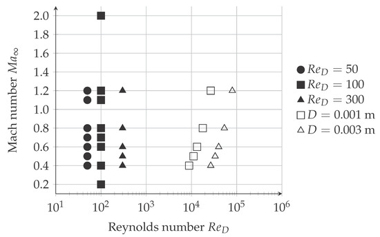
Figure 2. Simulation points at different Mach and Reynolds numbers, $M{a}_{\infty }$ and $R{e}_D$, for constant Reynolds number (black) and constant diameter (white).

3.1. Numerical Method and Model

The simulations were performed using the commercial software tool Ansys CFX 19.0. In Ansys CFX, the Navier–Stokes equations are solved using the Element-Based Finite-Volume Method. Depending on the Mach number $M{a}_{\infty }$ and whether the flow is stationary or transient, etc., the partial differential equations that are solved are elliptic, parabolic, hyperbolic or even of mixed-type.

The transport equations are solved in an implicit way. In general, the transient scheme of “Second Order Backward Euler” and the advection scheme of “High Resolution”, respectively, are chosen. The “High Resolution” advection scheme is based on the boundedness principles used by Barth and Jesperson [18]. The pressure–velocity coupling proposed by Rhie and Chow [19] and modified by Majumdar [20] is used.

The heat transfer is chosen to be “Total Energy”, which is necessary for high-speed flows at flow velocities u near the speed of sound a. Using “Total Energy”, the transport equation for total enthalpy $h^0$ is solved, which is related to the static enthalpy h according to Equation (8).

$$h^0=h+\frac{1}{2}{\overrightarrow{u}}^2$$

(8)

Turbulence is modelled using the Shear Stress Transport (SST) model. It is a suitable trade-off between quality and computational time. One of its strengths is the accuracy of the prediction of the onset and the amount of flow separation under adverse pressure gradients. In contrast with the Direct Numerical Simulation (DNS), in which the turbulent structures of all length scales are resolved with a fine computational mesh, all length scales are modelled in this turbulence model. For this reason, the flow variables are split into their time-averaged values and their fluctuating components and the Reynolds-Averaged Navier–Stokes (RANS) equations have to be solved. In order to do so, models for the computation of the Reynolds stresses and the Reynolds fluxes are provided. The SST turbulence model was first presented by Menter [21] and combines the advantages of the k-$\omega$ turbulence model near the wall and the k-$ϵ$ turbulence model in the bulk flow. Based on the distance of a node to the nearest wall, blending functions are used to ensure a smooth transition between the two models.

Because the near wall formulation determines the accuracy of the wall shear stress, “automatic wall functions” are used. Depending on the $y^{+}$-value, switching occurs between the low-Reynolds near wall approach and the wall-function approach, which is logarithmic for higher $y^{+}$-values. [22]

3.2. Description of the Computational Domain

Figure 3 shows the computation domain of the cylinder and its surroundings. Different computational domains with different values of $x_{\min }$, $x_{\max }$, $y_{\min }$ and $y_{\max }$ were carried out for the different simulation conditions depending on $R{e}_D$ and $M{a}_{\infty }$. This leads to various cylinder diameters D.

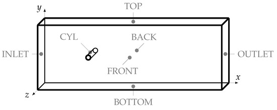
Figure 3. Computational domain with the locations of the boundary conditions in capital letters.

3.3. General Simulation Parameters

The geometries and the meshes were created with Ansys ICEM CFD. The simulations were performed as transient with a steady-state solution as the initial condition. To speed up the solving process, the steady-state solution of the laminar regimes was set up with a rotating cylinder $\mathsf{\Omega }=\frac{2·u_{\infty }}{D}$ in order to obtain unsteady behaviour in shorter time steps. This idea follows those proposed by Shirani [14] and Braza et al. [23]. Furthermore, simulations with coarser meshes were used as initial conditions, the final simulations were carried out with finer meshes. Three different considerations are made regarding the time step size $\Delta t$. Firstly, an estimation of the time step size based on the vortex shedding frequency f assuming $Str\approx 0.21$ is made with one oscillation period being resolved with 16 time steps. Secondly, the time step size is calculated from a mean cell dimension of the free stream according to $\Delta t\sim \frac{\Delta x_{\mathrm{cell}}}{u_{\infty }}$. Thirdly, the time step size can be calculated using the acoustic Courant number. Since the present work involves transonic conditions with velocities $u_{\infty }$ close to the speed of sound $a_{\infty }$, the time step size $\Delta t\sim \frac{\Delta x_{\mathrm{cell}}}{a_{\infty }}$ is of the same order of magnitude as the previously mentioned one. The time step $\Delta t\sim \frac{\Delta x_{\mathrm{cell}}}{u_{\infty }}$ was the smallest one in all the simulations; this one was chosen. The time steps $\Delta t$ of the final simulations lie in the range of micro- to nanoseconds.

3.4. Mesh Generation

Some phenomena of compressible flow are more strongly influenced by the selected flow region or the boundary conditions than others. For this reason, a combined geometry and mesh study was performed to assess and minimise the influence of the mesh and the geometry dimensions. It was carried out for different Mach numbers $M{a}_{\infty }$ and for the Reynolds number of $R{e}_D=100$, as well as the constant cylinder diameter of $D=0.003$ $\mathrm{m}$ in an iterative manner. The mesh was refined step by step and the relative deviations of $Str$, ${\overline{C}}_{\mathrm{D}}$ and $M{a}_{\max }$ were calculated between two meshes. If the relative deviation in these quantities of the respective mesh from the next finer mesh is less than 2.5 %, where most of the deviations are even below 1 %, then the mesh is considered to be sufficiently fine. The mesh quality of each mesh was determined according to the requirements in Table 2, where the minimum and maximum values over all the meshes are listed. Most of the criteria are within the required range, only a few cells exceed the criteria of the mesh expansion factor. Table 3 shows the result of the mesh study with the corresponding domain sizes and the number of cells for each simulation.

Table 2. Mesh quality requirements based on several criteria and min./max. values of all the meshes.

Criteria	Requirement	Min./Max. Value
Aspect ratio	<1000 “double precision” [24]	1.41 to 140.5
Orthogonal quality (numerical accuracy, robustness)	>1/3 [24], >0.1 [25]	0.72 to 1
Skewness	<0.95 [25]	0 to 0.5
Smoothness	1 to 1.5 [25]	1 to 1.47
Angle	20 to 160 [26]	45 to 134.4
Mesh expansion factor	<1.2	1 to 1.5

Table 3. Size of the computational domain (min. and max. values of x and y) and number of mesh cells for different simulations based on $R{e}_D$ and $M{a}_{\infty }$.

${\mathit{Re}}_{\mathit{D}}$	${\mathit{M}\mathit{a}}_{\mathit{\infty }}$	Range x	Range y	Number of Cells
50	0.4 to 1.1	$-50·D\le x\le 50·D$	$-50·D\le y\le 50·D$	323,304
	1.2			1,290,432
100	0.2 to 2.0	$-50·D\le x\le 50·D$	$-50·D\le y\le 50·D$	1,290,432
300	0.4 to 0.5	$-50·D\le x\le 50·D$	$-50·D\le y\le 50·D$	1,290,432
	0.6 to 0.8	$-25·D\le x\le 100·D$	$-25·D\le y\le 25·D$	3,547,380
	1.2	$-50·D\le x\le 50·D$	$-50·D\le y\le 50·D$	1,290,432
8890	0.4	$-50·D\le x\le 50·D$	$-50·D\le y\le 50·D$	1,307,732
11,100	0.5
13,300	0.6
17,800	0.8
26,700	1.2
26,700	0.4	$-25·D\le x\le 100·D$	$-25·D\le y\le 25·D$	3,547,380
33,400	0.5	$-50·D\le x\le 50·D$	$-50·D\le y\le 50·D$	1,307,732
40,000	0.6	$-25·D\le x\le 100·D$	$-25·D\le y\le 25·D$	3,547,380
53,400	0.8
80,000	1.2	$-50·D\le x\le 50·D$	$-50·D\le y\le 50·D$	1,307,732

The general mesh, which is shown in Figure 4, consists of sixteen mesh blocks with a square O-grid with an overall dimension of $3·D$ around the cylinder. A second O-grid within the first one was created to better resolve the boundary layer around the cylinder surface. It is ensured that the $y^{+}$-value is $y^{+}<300$ to model the boundary layer with automatic wall function. The $y^{+}$-value amounts to $5<y^{+}<35$ for the turbulent simulations. The z-direction is resolved with one cell; the dimension of this cell is scaled with the smallest cell dimension near the cylinder wall. The cell sizes in the x- and y-directions increase with increasing distance from the cylinder with a maximum growth rate of 1.2 to have a trade-off between computational time and accuracy.

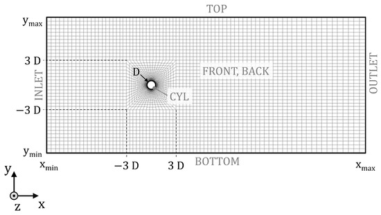
Figure 4. Domain and general mesh showing the dimensions of the mesh blocks and in capital letters the locations of the boundary conditions.

3.5. Boundary Conditions

The boundary conditions shown in Table 4 are given separately for $M{a}_{\infty }<1$ and $M{a}_{\infty }>1$. The pressures for the subsonic and supersonic simulations were set to $p=0\mathrm{bar}\left(\mathrm{g}\right)$ and $p=8\mathrm{bar}\left(\mathrm{g}\right)$, respectively.

Table 4. Boundary conditions for $M{a}_{\infty }<1$ and $M{a}_{\infty }>1$; positions of the boundary conditions according to Figure 3.

Position	Boundary Condition
	${\mathit{Ma}}_{\infty }<\mathbf{1}$	${\mathit{Ma}}_{\infty }>\mathbf{1}$
CYL	No slip wall
FRONT, BACK	Symmetry
INLET	$u_{\infty }$, T	p, $u_{\infty }$, T
OUTLET	p	Outlet
TOP, BOTTOM	Free slip wall	Outlet

4. Verification and Validation

In addition to the mesh and the parametrical study, the numerical procedure was verified and validated for selected cases of planar transonic flow situations. The Laval nozzle was used to analyse the flow phenomenon of the straight shock wave more precisely regarding the numerics. Furthermore, the results were validated with results from other investigations.

4.1. Laval Nozzle for Verification

The planar Laval nozzle with air assumed as ideal gas shown in Figure 5 was simulated for verification. The boundary conditions defined are either Dirichlet or Neumann boundary conditions, as shown in Figure 5. Symmetry boundary conditions were chosen in the direction perpendicular to the drawing plane and on the middle axis of the Laval nozzle, which are basically zero-gradient conditions. Different boundary conditions were specified for the wall in two simulations, no slip ($u=0$ ${\mathrm{m}/\mathrm{s}}^{-1}$) and free slip in order to analyse the influence of the wall on the flow phenomena. Three different meshes with 3125, 12,500 and 50,000 elements were used to investigate the influence of mesh resolution on the shock, where a sufficient mesh quality is ensured using the criteria listed in Table 2. The solver process is started with the advection schemes “Upwind” and “High Resolution”, respectively, for comparison purposes with a maximum number of 10,000 iterations.

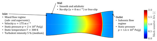
Figure 5. Planar Laval nozzle (length 0.84 m) coloured by the Mach number $Ma$ including the boundary conditions for the inlet, the outlet and the wall. The inlet (dimension of 0.14 m) of the Laval nozzle is on the left-hand side; the outlet (dimension of 0.17 m) is on the right-hand side. Only the upper half of the Laval nozzle is simulated resolved with 12,500 elements due to the x-axis symmetry.

One result of the Mach number $Ma$ from the CFD simulation of the Laval nozzle described above is shown in Figure 5. The subsonic flow from the inlet is accelerated to a Mach number of around 1.8 along the Laval nozzle. Further downstream follows a shock and a strong reduction of $Ma$ to about 0.6. Downstream, the flow is slightly decelerated until it finally reaches the outlet.

In a next step, the behaviour of the Mach number $Ma$ along the Laval nozzle is examined in more detail. In order to do so, Figure 6 shows $Ma$ along the central axis of the Laval nozzle for different simulation setups with the three different meshes. The result of a simplified calculation is also shown in black colour for comparison. For this calculation, the flow is assumed to be one-dimensional, steady-state, compressible and adiabatic with air as ideal gas and with a shock wave expansion which is infinitesimally small. It is an iterative calculation, whereby the exact shock position of $x=0.6979\mathrm{m}$ is calculated. Figure 6 shows two different curves for each simulation; these are the area-averaged Mach number over the respective position in blue colour and $Ma$ evaluated on the central axis of the Laval nozzle in red colour. The reason for this is the better comparability with the one-dimensional calculation. However, due to the two-dimensional simulation, comparability is only guaranteed to a limited extent. It is obvious that at $Ma$ on the central axis (red curves) the shock can be depicted more precisely with a finer mesh resolution. In the simulation with “High Resolution” and the free-slip wall, the shock occurs further downstream, which seems plausible. As a result of the higher-order advection scheme, the gradient at the shock position can be depicted better, resulting in a steeper curve. After the decrease of $Ma$ as a result of the shock, there is a non-physical undershoot. Compared to a higher-order scheme, the first-order scheme “Upwind” suffers from numerical diffusion. Therefore, the higher-order scheme “High Resolution” should be chosen in order to sufficiently resolve the shocks. In the case of the area-averaged curves, the gradient at the shock position is almost identical for the different mesh resolutions. The reason for that is, as Figure 5 shows, that the shock is not completely straight, it is curved. However, the shock position of the different meshes differs only slightly. Detailed analyses of the flow variables, such as pressure p, temperature T and the Mach number $Ma$ show that there are about eight to nine elements needed to resolve the shock. In reality, the extent of shock waves in the stream-wise direction amounts to only a few mean free paths of the molecules, so this must be taken into account.

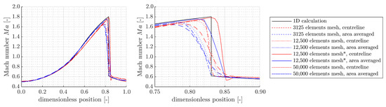
Figure 6. Mach number $Ma$ along the planar Laval nozzle from the one-dimensional calculation and the two-dimensional simulation results. Full range (left) and zoomed region of interest (right). The simulation results indicated with * were performed using a free-slip wall instead of a no-slip wall and an advection scheme of “High Resolution” instead of “Upwind”.

4.2. Validation with Literature

In addition to the verification using the Laval nozzle, some points were also simulated based on $M{a}_{\infty }$ and $R{e}_D$, for which results from other work [17,27,28] are available. The compressible and the incompressible flow around a planar circular cylinder at $R{e}_D=100$ and $M{a}_{\infty }=0.2$ and the compressible flow at $R{e}_D=100$ and $M{a}_{\infty }=2$ are investigated.

Figure 7a,b show the velocity component $u_x$ of the compressible flow at $R{e}_D=100$ and $M{a}_{\infty }=0.2$, in which the advection schemes “Upwind” and “High Resolution” are compared with each other. The results show that a higher-order advection scheme is necessary for the adequate prediction of the periodic vortex shedding, a so-called Kármán vortex street. In addition, Table 5 shows the time-averaged drag coefficient ${\overline{C}}_{\mathrm{D}}$ and the Strouhal number $Str$ for the incompressible and compressible cases, including a comparison with the literature. A good agreement of ${\overline{C}}_{\mathrm{D}}$ and $Str$ with the literature can be seen with a maximum deviation of approximately 2% and 4%, respectively.

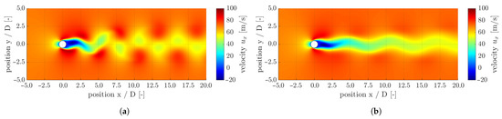
Figure 7. Transient result of velocity in x-direction $u_x$ at $R{e}_D=100$ and $M{a}_{\infty }=0.2$ with a time step size of ${10}^{-8}$ s. (a) Advection scheme “High Resolution”; (b) Advection scheme “Upwind”.

Table 5. Comparison of the Strouhal number $Str$ and the time-averaged drag coefficient ${\overline{C}}_{\mathrm{D}}$ at $R{e}_D=100$ and $M{a}_{\infty }=0.2$ with other studies [17,27,28].

	Compressibility	$\mathit{Str}$	${\overline{\mathit{C}}}_{\mathbf{D}}$
This study	incompressible	0.176	1.396
This study	compressible	0.162	1.419
Burbeau and Sagaut [17] and Lesaint and Raviart [27]	incompressible	0.173	1.411
Burbeau and Sagaut [27] and Oden Tinsley et al. [28]	compressible	0.165	1.370

In addition, the supersonic flow at $R{e}_D=100$ and $M{a}_{\infty }=2$ was also considered. For this purpose, the boundary conditions are chosen according to Table 4. Figure 8a shows the Mach number $Ma$ distribution, in which the detached shock position corresponds very precisely to that from Burbeau and Sagaut [17] (dashed black line). Figure 8b shows a simulation result with extended flow area in the positive x- and y-axis directions. The symmetry is assumed in the simulation with respect to the x-axis, because the flow in Figure 8b is also symmetric with respect to the x-axis. The flow phenomena at $R{e}_D=100$ and $M{a}_{\infty }=2$ can be clearly seen in Figure 8a,b. A detached shock forms upstream of the cylinder. This detached shock turns into a Mach cone along the shock front with increasing distance in the y-direction. The opening angle of $\alpha ={32}^{\circ }$ from Figure 8b agrees well with the theoretical angle of $\alpha ={30}^{\circ }$ according to Equation (10); for more details, see Section 5.4.

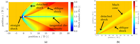
Figure 8. Mach number $Ma$ distribution showing the flow phenomena at $R{e}_D=100$ and $M{a}_{\infty }=2$ for two geometries. (a) Shock wave position from Burbeau and Sagaut [17] (dashed line); (b) Extended geometry.

In Figure 8a, a weak reflection of the detached shock at the boundary conditions in the y-direction downstream from around $x/D=7$ can also be seen. In comparison to Figure 8b, the influence of the boundary condition is clearly visible. For this reason, when simulating the flow around the planar circular cylinder, it must be ensured that the limitation of the flow region in the y-direction is chosen sufficiently. In addition to the detached shock, two oblique shocks form downstream of the cylinder or obliquely away from the cylinder. Analogously to the detached shock, this is followed by an abrupt change or a discontinuity of the flow variables. A wake with a very small velocity $u\approx 0$ forms downstream of the cylinder. This wake is separated from the rest of the flow area by a tangential discontinuity; for more details, see Section 5.1.

5. Results and Discussion

In the first subsection of this chapter, the way different flow phenomena are identified is described. The eight flow regimes obtained are then described in a general way and classified, based on $M{a}_{\infty }$ and $R{e}_D$. The flow structures of the regimes are discussed in more detail and compared to other authors. After that, the straight and the $\lambda$ shocks are evaluated. Finally, the critical Mach number $M{a}_{\mathrm{crit}}$, the Strouhal number $Str$, the drag coefficient ${\overline{C}}_{\mathrm{D}}$ and the polar diagrams are presented.

5.1. Identification of Flow Phenomena

Inspired by the experimental Schlieren flow visualisation techniques, the modulus of the dimensionless density gradient $\frac{D·\left|\nabla \rho \right|}{{\rho }_{\infty }^0}$ is used to visualise all relevant flow phenomena.

Various shock waves can be observed in compressible flows such as detached shocks, normal shocks, oblique shocks and $\lambda$ shocks. Shocks are irreversible discontinuities in the flow variables over a few mean free-path lengths of the molecules. If the plane of the discontinuity is perpendicular to the flow or the streamlines, it is a straight shock wave. The streamlines are not deflected and the flow is supersonic upstream of the shock and subsonic downstream. In the case of an oblique shock, however, the streamlines are kinked and the normal component of the velocity is supersonic upstream of the shock and subsonic downstream. The magnitude of the tangential velocity component is constant across the shock and the flow downstream of the shock can be either subsonic or supersonic. In addition to the density gradient, shocks can be identified by a discontinuous change in other flow variables. An example is the Mach number $Ma$ shown in Figure 9a, which decreases over the detached shock as well as the oblique shock (Figure 10). Across the detached shock, the flow regime changes from supersonic to subsonic and over the oblique shock from supersonic to a lower velocity in the supersonic range. The streamlines in Figure 9a are kinked across the shock waves away from the x-axis, but not on the symmetry axis in the y-direction, where the detached shock is normal to the streamlines. Furthermore, the pressure p increases across both the detached and the oblique shocks, as shown in Figure 9c. As can be seen in Figure 9d, there is a discontinuous reduction in the total pressure $p^0$ across the shocks.

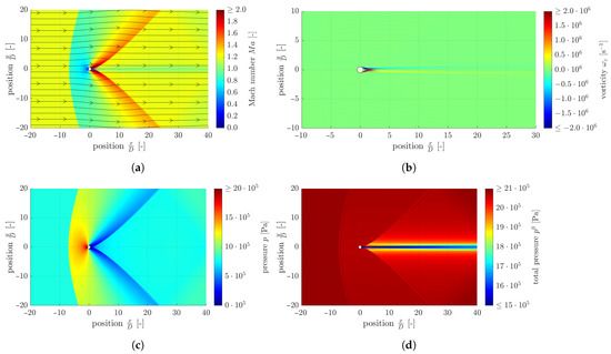
Figure 9. Shocks and tangential discontinuities at $M{a}_{\infty }=1.2$ and $R{e}_D=$26,700 visualised by $Ma$, ${\omega }_z$, p and $p^0$. (a) Mach number $Ma$ field with streamlines in black colour; (b) Vorticity component ${\omega }_z$ distribution; (c) Pressure p distribution; (d) Total pressure $p^0$ distribution.

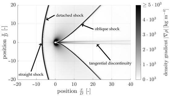
Figure 10. Density gradient $\left|\nabla \rho \right|$ at $M{a}_{\infty }=1.2$ and $R{e}_D=26,700$ showing the different phenomena.

In the wake of the cylinder, a detachment forms at $M{a}_{\infty }=1.2$ and $R{e}_D=26,700$, which is characterised by two converging shear layers further downstream of the cylinder. There is no mass flow across this tangential discontinuity (Figure 10) and because of that the normal velocity component on both sides of the tangential discontinuity must be zero. Therefore, the streamlines are parallel in the area of the tangential discontinuity, which can be seen in Figure 9a. As shown in Figure 9a, there is a discontinuity in the Mach number $Ma$ and in the tangential velocity component. Due to this change in the tangential velocity, a theoretically diverging vorticity $\omega$ (see Equation (9)) results, which can be used to identify the tangential discontinuity. Due to the mesh resolution, which is finite, there is no abrupt discontinuity in the tangential velocity component; however, the value of the corresponding vorticity component still becomes very large.

$$\overrightarrow{\omega }=\overrightarrow{\nabla }\times \overrightarrow{u}$$

(9)

Across such a tangential discontinuity, the pressure p, however, must be continuous (see Figure 9c). The total pressure $p^0$ (Figure 9d) in turn may be and in general will be discontinuous, as can be concluded from the momentum balance.

The question arises, how the vortices can be distinguished from other flow phenomena. The z-component of the vorticity ${\omega }_z$ is shown in Figure 11a, whereby the left-turning and right-turning vortices have a different sign. In contrast to the tangential discontinuity, the streamlines cross areas of different orders of magnitude of the vorticity. Vortices are rather smeared out compared to shocks and tangential discontinuities. In addition, vortices are decently visible in the swirling strength $\zeta$, as shown in Figure 11b (the swirling strength $\zeta$ denotes the imaginary part of the pair of complex-conjugated eigenvalues of the velocity gradient tensor. Thus, in the case where the velocity gradient tensor is symmetric, the swirling strength is zero).

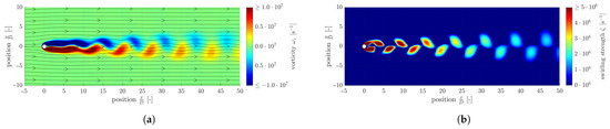
Figure 11. Shedding vortices at $M{a}_{\infty }=0.4$ and $R{e}_D=50$ visualised by ${\omega }_z$ and $\zeta$; (a) Vorticity component ${\omega }_z$; (b) Swirling strength $\zeta$.

5.2. Classification of Flow Regimes

The eight flow regimes, denoted by (a) to (h), are shown in Figure 12 and compared to the incompressible regimes from Schlichting and Gersten [1]; incompressible flow is assumed as $M{a}_{\infty }<0.3$. The occurring compressible regimes (a) to (c) at $R{e}_D=50$ to 100 and $0.2\le M{a}_{\infty }\le 0.8$ are similar to the incompressible regimes. It is observed that subsonic $M{a}_{\infty }$ of $0.6\le M{a}_{\infty }\le 0.8$ suppress the vortices in the wake of the cylinder for $R{e}_D=50$, whereas the incompressible flow regime at $R{e}_D=50$ shows an onset of the Kármán vortex street. Increasing $R{e}_D$ with subsonic $0.4\le M{a}_{\infty }\le 0.6$ and $R{e}_D\ge 300$ leads to regime (d), which is similar to the incompressible subcritical regime. In contrast, sound wave propagation is shown in compressible flow. The regimes (e) to (h) differ from the incompressible regimes, because the $M{a}_{\infty }$ is far away enough from the incompressible flow. For $M{a}_{\infty }=0.8$ and $R{e}_D\ge 300$, $\lambda$ shocks as well as vortices are formed. In the supersonic regimes, it is observed that a detached shock upstream of the cylinder and two oblique shocks downstream of the cylinder are formed. In addition, for $50\le R{e}_D\le 300$ and $1.1\le M{a}_{\infty }\le 2$, regime (g) occurs and vortices in the wake of the cylinder are formed. For higher Mach numbers $M{a}_{\infty }$, the wake of the cylinder is steady and symmetric; this corresponds to regime (h).

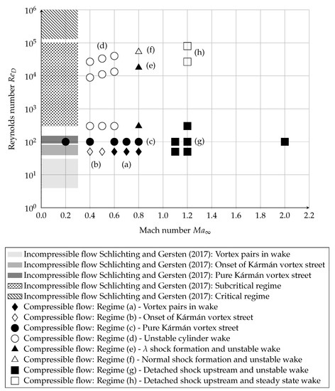
Figure 12. Flow regimes based on $R{e}_D$ and $M{a}_{\infty }$ occurring in the compressible flow compared to the results of Schlichting and Gersten [1].

5.3. In-Depth Analysis of the Eight Flow Regimes

Basically, the dimensionless density gradient $\frac{D·\left|\nabla \rho \right|}{{\rho }_{\infty }^0}$ consists of the density gradient $\left|\nabla \rho \right|$ multiplied with the cylinder diameter D divided by an averaged total free stream density ${\rho }_{\infty }^0$. Typical results including only the most interesting areas of the simulation domain are shown for the different regimes in Figure 13, Figure 14, Figure 15, Figure 16, Figure 17, Figure 18, Figure 19, Figure 20 and Figure 21.

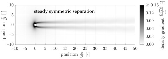
Figure 13. Regime (a), example $R{e}_D=50$ and $M{a}_{\infty }=0.6$, distribution of $\frac{D·\left|\nabla \rho \right|}{{\rho }_{\infty }^0}$.

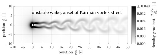
Figure 14. Regime (b), example $R{e}_D=50$ and $M{a}_{\infty }=0.4$, distribution of $\frac{D·\left|\nabla \rho \right|}{{\rho }_{\infty }^0}$.

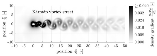
Figure 15. Regime (c), example $R{e}_D=100$ and $M{a}_{\infty }=0.4$, distribution of $\frac{D·\left|\nabla \rho \right|}{{\rho }_{\infty }^0}$.

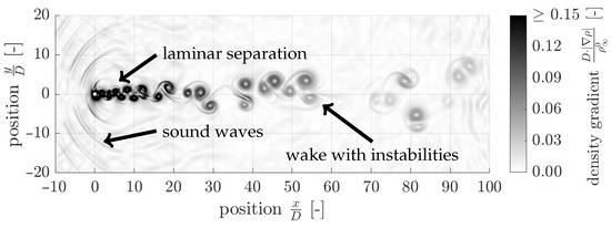
Figure 16. Regime (d), example $R{e}_D=300$ and $M{a}_{\infty }=0.6$, distribution of $\frac{D·\left|\nabla \rho \right|}{{\rho }_{\infty }^0}$.

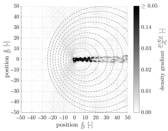
Figure 17. Sound wave propagation, $R{e}_D=300$ and $M{a}_{\infty }=0.5$, distribution of $\frac{D·\left|\nabla \rho \right|}{{\rho }_{\infty }^0}$.

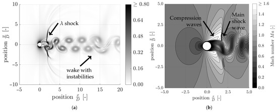
Figure 18. Regime (e), example $R{e}_D=300$ and $M{a}_{\infty }=0.8$. (a) Distribution of $\frac{D·\left|\nabla \rho \right|}{{\rho }_{\infty }^0}$; (b) Contour plot of the Mach number $Ma$.

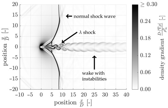
Figure 19. Regime (f), example $R{e}_D=$ 53,400 and $M{a}_{\infty }=0.8$, distribution of $\frac{D·\left|\nabla \rho \right|}{{\rho }_{\infty }^0}$.

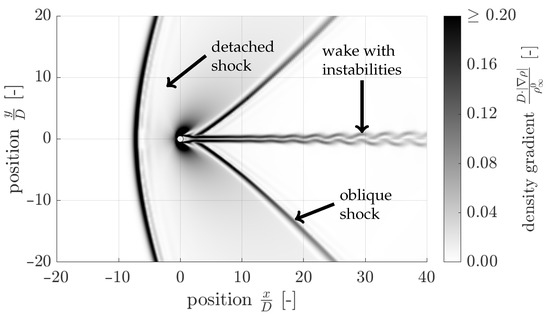
Figure 20. Regime (g), example $R{e}_D=100$ and $M{a}_{\infty }=1.2$, distribution of $\frac{D·\left|\nabla \rho \right|}{{\rho }_{\infty }^0}$.

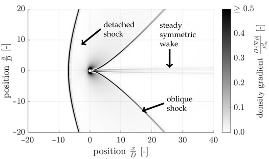
Figure 21. Regime (h), example $R{e}_D=$ 26,700 and $M{a}_{\infty }=1.2$, distribution of $\frac{D·\left|\nabla \rho \right|}{{\rho }_{\infty }^0}$.

Regime (a) in Figure 13 belongs to a steady symmetric separation downstream of the cylinder. The flow detaches symmetrically on the upper and lower sides of the cylinder surface, whereby a shear layer (tangential discontinuity) forms due to the two different tangential velocities. This is in good agreement with the findings from Nagata et al. [6], where the experimental investigation for $M{a}_{\infty }=0.2$ to $0.5$ at $R{e}_D=1000$ (slightly larger $R{e}_D$ compared to Figure 13) shows very similar behaviour. The shear layers that form at the detachment point are more pronounced at larger $M{a}_{\infty }$ due to the increasing density gradient $\left|\nabla \rho \right|$. Furthermore, Nagata et al. [6] investigate the dependence on the Reynolds number $R{e}_D$ in the range from 1000 to 5000 at $M{a}_{\infty }=0.5$. The flow detaches at the poles of the cylinder surface and a backflow area forms immediately downstream of the cylinder, which becomes more unstable and shorter with increasing $R{e}_D$, the flow starts to develop swirl.

Regime (b) is shown in Figure 14, where in comparison to the stable wake in Figure 13, an unstable wake with periodical vortex shedding forms. The vortex street is not fully developed; it is an onset of a Kármán vortex street. This flow regime can be validated using the results of Canuto and Taira [12], whereby the simulation results at $M{a}_{\infty }=0,0.3,\mathrm{and}0.5$ and $R{e}_D=50$ show less pronounced vortices with increasing $M{a}_{\infty }$. In particular, when looking at Figure 13 and Figure 14, it is noticeable that with a Reynolds number of $R{e}_D=50$ and $M{a}_{\infty }=0.4$, an unstable wake with periodic vortices results, whereas an increase in the Mach number to $M{a}_{\infty }=0.6$ results in a symmetrical, stationary cylinder wake. In the investigations by Canuto and Taira [12], the maximum Mach number is $M{a}_{\infty }=0.5$, with weak eddies still occurring, which could also be observed in this study.

Regime (c) in Figure 15 shows a periodical vortex shedding, a so-called Kármán vortex street, where the oscillation amplitude of the vortices is growing downstream of the cylinder over approximately the first four pairs of vortices. The Kármán vortex street can be compared with the results from Van Dyke [29] (Figures 94 to 96) for the Reynolds numbers $R{e}_D=105,140,$ and 200. Despite the incompressible flow, the qualitative pattern fits with the behaviour shown in Figure 15. Comparing the vortices in Figure 15 with Figure 14, it can be noticed that an increase in $R{e}_D$ from 50 to 100 at a constant Mach number of $M{a}_{\infty }=0.4$ leads to stronger vortices. These vortices turn more and more into a Kármán vortex street. This influence of the Reynolds number is studied by Canuto and Taira [12] using Reynolds numbers of $R{e}_D=60,80,$ and 100, where the vortices are also more pronounced with higher $R{e}_D$ and the distance between two consecutive vortices decreases. The results in Figure 14 and Figure 15 agree very well with the experimental results of Canuto and Taira [12] in a qualitative manner.

Regime (d) in Figure 16 is similar to regime (c); vortices are shed periodically. However, the wake further downstream of the cylinder is unstable and there is a sound wave propagation. The sound waves are present in the compressible simulations for the Reynolds numbers $100\le R{e}_D\le$ 80,000 with a subsonic free stream Mach number $0.4\le M{a}_{\infty }\le 0.8$. Müller [30] found that each time a vortex is shed from the cylinder, a sound wave is emitted. Further numerical investigations on the sound wave propagation from a circular cylinder in a wide range of Reynolds numbers for $R{e}_D=150$ and $M{a}_{\infty }=0.1\mathrm{and}0.2$ [31,31], $R{e}_D=200$ and $M{a}_{\infty }=0.3$ [32], $R{e}_D=1000$ and $M{a}_{\infty }=0.27$ [33], as well as $R{e}_D=1.58\times {10}^4$ [34] are presented in the literature. The results of Dumbser [35] at $R{e}_D=150$ and $M{a}_{\infty }=0.2$ show a flow behaviour very similar to Figure 16. Although no sound waves are observed in this study at low Mach numbers, below $M{a}_{\infty }=0.4$, the results of Dumbser [35] make regime (d) appear more plausible. The reason that no sound waves can be observed might be the small density gradient or the too small flow domain for the prediction of sound waves. However, since the results from Khalili et al. [31], Dumbser [35] and Müller [30] are obtained using high-order numerical simulations, it is questionable whether the advection scheme “High Resolution” can sufficiently predict the sound waves. Due to this, the phenomena are analysed as in Figure 17, which shows the example of $R{e}_D=300$ and $M{a}_{\infty }=0.5$. The so-called Doppler effect occurs. Thereby, the sound source’s location is almost constant and lies near the cylinder. The wave fronts upstream of the sound source are compressed and those downstream are thinned. The thinning and compressing increase with increasing Mach numbers $M{a}_{\infty }$ until $M{a}_{\infty }=1$ is reached. Some representative points are chosen for every sound wave and circles with centre on the x-axis are fitted through the points in Figure 17. Finally, the Mach number can be calculated from the difference in the circle centres and radii $Ma=\frac{u}{a}=\frac{\Delta x}{\Delta r}$. Using the differences of each circle to the first one and calculating the arithmetic mean, a Mach number of $Ma=0.48$ is obtained. This Mach number has a relative deviation of $-4\%$ compared to the free stream Mach number $M{a}_{\infty }=0.5$.

Regime (e) is shown in Figure 18a and consists of a wake with instabilities downstream of the cylinder and two $\lambda$ shocks immediately downstream of the cylinder. Regime (f) in Figure 19 basically is analogous to regime (e), but the $\lambda$ shocks turn into a normal shock wave further away from the cylinder. However, the transition of the $\lambda$ shocks into normal shocks might be a result of an intersection with the boundary conditions. Various investigations from other works at higher Reynolds numbers $R{e}_D$, such as Linn and Awruch [16] at $R{e}_D=5\times {10}^5$, support this conclusion. Therefore, it is assumed that regime (e) occurs in a wide range of $R{e}_D\ge 300$ at $M{a}_{\infty }=0.8$. Figure 18b shows the contour diagram of the simulation with $R{e}_D=300$ and $M{a}_{\infty }=0.8$; at this point, several phenomena of interest occur. Starting from the free stream, the fluid slows down on the symmetry x-axis owing to the stagnation point. Above and below the x-axis, the fluid is accelerated. Downstream of the cylinder, two $\lambda$ shocks occur, which consist of compression waves and a main shock wave. Compression waves lead to a continuous increase in the Mach number $Ma$; this is indicated with the Contour lines, which are parallel to each other. Through the main shock wave, the $Ma$ is decreased from supersonic to subsonic regime, passing multiple contour lines. The $\lambda$ shocks in Figure 19 interact with the flow separation. Bobenrieth Miserda and Leal [9] investigated these complex viscous shock interactions using basically a Detached Eddy Simulation. They observed $\lambda$ shocks associated with the boundary layer separation point, quasi-straight shocks that are normal to shear layers and connecting shocks between vortices at $M{a}_{\infty }=0.8$ and $R{e}_D=$ 500,000 (higher $R{e}_D$ compared to this study). The overall flow behaviour of Bobenrieth Miserda and Leal [9] is similar to this study with the development of the two $\lambda$ shocks and the vortex street. However, the simulation results of Bobenrieth Miserda and Leal [9] show the flow phenomena in more detail, because of the numerical method and the higher mesh resolution. Comparable experimental results can also be found in the study of Van Dyke [29] (Figure 222) for $M{a}_{\infty }=0.8,0.9,0.95,\mathrm{and}0.98$ and a small Reynolds number $R{e}_D$. The results of Van Dyke [29] at $M{a}_{\infty }=0.8$ are identical to the results shown in Figure 18a and therefore the simulation results seem plausible. The experimental results found by Rodriguez [4] support the simulation results in Figure 18a as well, where the two $\lambda$ shocks and the instabilities downstream of the cylinder were found at $M{a}_{\infty }=0.75$ and $R{e}_D={10}^5$.

Regime (g) in Figure 20 shows a detached shock upstream of the cylinder, two oblique shocks downstream of the cylinder and a wake with vortices. The only difference between the flow situation at a higher Reynolds number of $R{e}_D=$ 26,700 in Figure 21 is the cylinder wake which is unstable with the lower Reynolds number of $R{e}_D=100$. Because of the identical Mach numbers $M{a}_{\infty }=1.2$, the oblique shock upstream of the cylinder is equal in both regimes (g) and (h), which seems plausible.

Regime (h) shown in Figure 21 is similar compared to regime (g), but there are no instabilities in the cylinder’s wake, as it is steady and symmetric. Because of the difference in the tangential velocities of the cylinder wake and the surrounding fluid, a tangential discontinuity is formed. This shear layer can be seen in the density gradient above and below the axis of symmetry in the y-direction downstream of the cylinder; there is no fluid passing these shear layers. Numerical results similar to regime (h) are obtained by de Tullio et al. [36], where $M{a}_{\infty }=1.7$ and $R{e}_D=$ 200,000 is investigated. However, $M{a}_{\infty }$ and $R{e}_D$ are higher compared to Figure 21. Despite this, the flow phenomena are very similar, which leads to the conclusion that this regime extends over a much larger range of Mach and Reynolds numbers. The flow phenomena of a detached shock upstream of the cylinder, the supersonic flow region between the cylinder, the detached shock, the subsonic recirculation region behind the cylinder and the two symmetrical oblique shocks, which are formed at the end of the recirculation region, are present in both the study from de Tullio et al. [36] and Figure 21. Obviously, an increase in the Mach number $M{a}_{\infty }$ leads to a higher curvature of the detached shock. Hinman et al. [37] performed numerical simulations at an even higher Mach number $M{a}_{\infty }=10$ and $R{e}_D=5.5\times {10}^4$, where the flow structure is somehow similar compared to Figure 21. However, there are noticeable differences in the flow structure, namely the lid separation shock, which connects the recirculation region with the oblique shock and there is more curvature in the detached shock due to the high Mach number.

5.4. Analysis of the Shock Waves

For Mach numbers $M{a}_{\infty }>1.0$, a detached shock is formed upstream of the cylinder. This shock consists of three different phenomena. Near the cylinder symmetry x-axis, an oblique shock is formed. Further away from the cylinder, a weaker oblique shock turns into a Mach cone, whose angle $\alpha$ can be calculated with Equation (10).

$$sin\left(\alpha \right)=\frac{1}{Ma}$$

(10)

Figure 22a shows this situation for $M{a}_{\infty }=1.2$ and $R{e}_D=100$. However, the shock angle of ${65}^{\circ }$ is larger than the angle of the Mach cone of $\alpha =56.4^{\circ }$. This is due to the fact that the geometry is not sufficiently large to depict the transition to the Mach cone. Different calculations of the normal shock wave on the x-axis have been done. The state upstream of the shock is indicated as 1 and the state downstream of the shock is indicated as 2. The simulation quantities were compared to the ones calculated from the theory. The results are shown in Table 6 and fit well with the calculations, the maximum deviation is about $-4\%$.

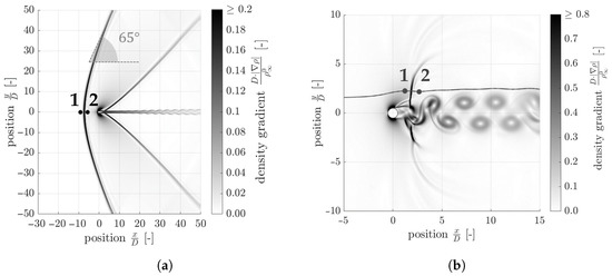
Figure 22. Analysis of shocks, distribution of $\frac{D·\left|\nabla \rho \right|}{{\rho }_{\infty }^0}$. The states upstream and downstream of the shock are indicated as 1 and 2. (a) $R{e}_D=100$ and $M{a}_{\infty }=1.2$, detached shock; (b) $R{e}_D=300$ and $M{a}_{\infty }=0.8$, $\lambda$ shock.

Table 6. Analysis of the detached shock for $R{e}_D=100$ and $M{a}_{\infty }=1.2$.

Quantity	Calculation	Simulation
$M{a}_1$	1.200	1.1999
$M{a}_2$	0.8422	0.8082
$\raisebox{1ex}{$p_2$}\!\left/ \!\raisebox{-1ex}{$p_1$}\right.$	1.5133	1.5675
$\raisebox{1ex}{$T_2$}\!\left/ \!\raisebox{-1ex}{$T_1$}\right.$	1.1280	1.1392
$\raisebox{1ex}{$p_2^0$}\!\left/ \!\raisebox{-1ex}{$p_1^0$}\right.$	0.9928	0.9936
$\raisebox{1ex}{${\rho }_2$}\!\left/ \!\raisebox{-1ex}{${\rho }_1$}\right.$	1.3416	1.3760
$\raisebox{1ex}{$u_2$}\!\left/ \!\raisebox{-1ex}{$u_1$}\right.$	0.7454	0.7189
$\raisebox{1ex}{$T_2^0$}\!\left/ \!\raisebox{-1ex}{$T_1^0$}\right.$	1.0000	1.0000

In addition, the $\lambda$-shock wave is analysed in a similar way for the simulation with $R{e}_D=300$ and $M{a}_{\infty }=0.8$. The flow regime as well as the states upstream and downstream of the shock are shown in Figure 22b. The calculations in Table 7 show that the simulation results fit well with the calculations. The maximum deviation is about −7.6%. The calculation of the different quantities shown in Table 7 is based on the upstream Mach number $M{a}_{\infty }=1.1258$ from the simulation results.

Table 7. Analysis of the $\lambda$ shock for $R{e}_D=300$ and $M{a}_{\infty }=0.8$.

Quantity	Calculation	Simulation
$M{a}_2$	0.8081	0.8102
$\raisebox{1ex}{$p_2$}\!\left/ \!\raisebox{-1ex}{$p_1$}\right.$	1.6801	1.5522
$\raisebox{1ex}{$T_2$}\!\left/ \!\raisebox{-1ex}{$T_1$}\right.$	1.1645	1.1403
$\raisebox{1ex}{$p_2^0$}\!\left/ \!\raisebox{-1ex}{$p_1^0$}\right.$	0.9859	0.9122
$\raisebox{1ex}{${\rho }_2$}\!\left/ \!\raisebox{-1ex}{${\rho }_1$}\right.$	1.4428	1.3613
$\raisebox{1ex}{$T_2^0$}\!\left/ \!\raisebox{-1ex}{$T_1^0$}\right.$	1.0000	0.9797

The Mach number downstream of the shock $M{a}_2$ can be calculated from the Mach number upstream of the shock $M{a}_1$ and the heat capacity ratio $\kappa =1.4$ for air.

$$M{a}_2^2=\frac{M{a}_1^2+\frac{2}{\kappa -1}}{\frac{2\kappa }{\kappa -1}M{a}_1^2-1}$$

(11)

The pressure ratio $\frac{p_2}{p_1}$ is calculated from the two Mach numbers $M{a}_1$ and $M{a}_2$ and the heat capacity ratio $\kappa$ as follows.

$$\frac{p_2}{p_1}=\frac{1+\kappa M{a}_1^2}{1+\kappa M{a}_2^2}$$

(12)

5.5. Critical Mach Number

The critical Mach number of the inflow $M{a}_{\mathrm{crit}}$ shown in Figure 23 was determined. This corresponds to the lowest Mach number of the inflow $M{a}_{\infty }$, at which the flow near the cylinder reaches the speed of sound a. Polhamus [38] discovered the critical Mach number for very large Reynolds numbers $R{e}_D\to \infty$ to be $M{a}_{\mathrm{crit}}=0.4$. This agrees with the critical Mach number found in this study at a Reynolds number of $R{e}_D=$ 26,683.

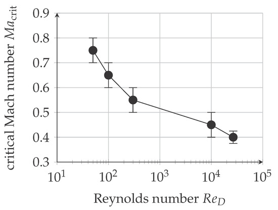
Figure 23. Critical Mach number $M{a}_{\mathrm{crit}}$ vs. Reynolds number $R{e}_D$.

5.6. Strouhal Number and Drag Coefficient

Table 8 shows an overview for the Strouhal number $Str$ and the mean drag coefficient ${\overline{C}}_{\mathrm{D}}$ of all simulation points; the Strouhal numbers are in the range of $0.1<Str<0.25$.

Table 8. Mean drag coefficient ${\overline{C}}_{\mathrm{D}}$ and Strouhal number $Str$.

${\mathit{Re}}_{\mathit{D}}$	${\mathit{Ma}}_{\mathit{\infty }}$	${\overline{\mathit{C}}}_{\mathbf{D}}$	$\mathit{Str}$
50	0.4	1.471	0.1143
	0.5	1.517	0.1080
	0.6	1.609	0.1075
	0.7	1.760
	0.8	2.069
	1.1	14.43	0.2128
	1.2	13.85	0.2279
100	0.2	1.319	0.1582
	0.4	1.410	0.1565
	0.6	1.648	0.1559
	0.7	1.847	0.1550
	0.8	1.877	0.1383
	1.1	13.822	0.2378
	1.2	13.453	0.2408
	2.0	12.970
300	0.4	1.483	0.1983
	0.5	1.623	0.2048
	0.6	1.781	0.2083
	0.8	2.380	0.2238
	1.2	13.46	0.2444
8890	0.4	1.603
11,100	0.5	1.726
13,300	0.6	1.834
17,800	0.8	1.860
26,700	1.2	14.145
26,700	0.4	1.614
33,400	0.5	1.717
40,000	0.6	1.873
53,400	0.8	2.171
80,000	1.2	13.808

Drag forces $F_{\mathrm{D}}$ occur in flows around objects and act opposite to the relative motion of the object with respect to the surrounding fluid. $F_{\mathrm{D}}$ basically consists of three forces: pressure drag, friction drag and wave drag. The friction drag is produced by the viscous momentum exchange; in addition, the drag force corresponds to the sum of all forces parallel to the flow. The wave drag is created when the velocity is close to the speed of sound a, which means the Mach number $M{a}_{\infty }$ exceeds the critical Mach number $M{a}_{\mathrm{crit}}$. Reaching the critical Mach number $M{a}_{\mathrm{crit}}$ leads to an increase in the mean drag coefficient ${\overline{C}}_{\mathrm{D}}$.

For the subsonic regimes, the mean drag coefficient lies in the range of $1.3<{\overline{C}}_{\mathrm{D}}<1.61$. For higher $M{a}_{\infty }$ in the transonic regimes, which means where the critical Mach number $M{a}_{\mathrm{crit}}$ is reached, the wave drag increases and the mean drag coefficient is in the range of $1.6<{\overline{C}}_{\mathrm{D}}<2.5$. Increasing the free stream Mach number to supersonic leads to very large ${\overline{C}}_{\mathrm{D}}$ of $12.5<{\overline{C}}_{\mathrm{D}}<14.5$; the reason for this is the compression fronts which lead to higher wave drag. The wave drag then decreases again in the supersonic range. The values of the drag coefficient ${\overline{C}}_{\mathrm{D}}$ and the Strouhal number $Str$ for $R{e}_D=50$ to 100 in a Mach number range $0\le M{a}_{\infty }\le 0.5$ are in good agreement with the values from Canuto and Taira [12].

5.7. Polar Diagrams

So-called polar diagrams, i.e., the lift coefficient $C_{\mathrm{L}}$ versus the drag coefficient $C_{\mathrm{D}}$ plotted, were evaluated. In some cases, the polar diagrams correspond to a closed curve, so-called Lissajous figures. In this case, the oscillations correspond to a single respectively finite number of frequencies involved. The frequency ratio as well as the phase shift can be determined analysing these closed curves. For the Kármán vortex street or similar phenomena, the drag coefficient $C_{\mathrm{D}}$ oscillates at double the frequency of the lift coefficient $C_{\mathrm{L}}$. This confirms the rough idea that the drag is basically a quadratic effect compared with lift, in agreement with the fact that drag is generally positive, whereas lift can be of either sign. For some simulation points, especially when vortex shedding occurs in the subsonic and supersonic regimes, closed curves are observed; typical results are shown in Figure 24a–d. Figure 24a corresponds to the subsonic simulation at $R{e}_D=100$ and $M{a}_{\infty }=0.4$ with the phenomena shown in Figure 15. The Lissajous figure shows that the lift coefficient $C_{\mathrm{L}}$ oscillates at half the frequency of the drag coefficient $C_{\mathrm{D}}$. The phase shift of the drag coefficient $C_{\mathrm{D}}$ is $\frac{\pi }{4}$ and $\frac{3·\pi }{4}$, respectively. Figure 24b shows the supersonic simulation point $R{e}_D=100$ and $M{a}_{\infty }=1.2$, the corresponding flow phenomena are shown in Figure 20. The frequency ratio is equal to Figure 24a; the phase shift of the drag coefficient $C_{\mathrm{D}}$ is $\frac{5·\pi }{4}$ and $\frac{7·\pi }{4}$, respectively. Figure 24c shows the transonic simulation point $R{e}_D=300$ and $M{a}_{\infty }=0.6$, related to the flow regime in Figure 16. The frequency ratio is equal to the previous Figure 24a,b; the phase shift of the drag coefficient $C_{\mathrm{D}}$ is $\frac{\pi }{2}$. Figure 24d shows the supersonic simulation point $R{e}_D=$ 13,300 and $M{a}_{\infty }=0.6$ and Figure 25 shows the corresponding flow phenomena in the distribution of the dimensionless density gradient $\frac{D·\left|\nabla \rho \right|}{{\rho }_{\infty }^0}$. Looking at the density gradient, the phenomena sound waves and vortex shedding are observed. However, the vortices shed randomly, which does not lead to a closed curve in the polar diagram. That means that several frequencies are involved in the oscillations. These random oscillations are observed for all the high Reynolds numbers $R{e}_D$ where the flow is turbulent.

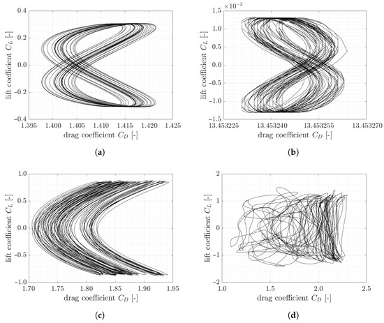
Figure 24. Polar diagrams. (a) $R{e}_D=100$ and $M{a}_{\infty }=0.4$; (b) $R{e}_D=100$ and $M{a}_{\infty }=1.2$; (c) $R{e}_D=300$ and $M{a}_{\infty }=0.6$; (d) $R{e}_D=$ 13,300 and $M{a}_{\infty }=0.6$.

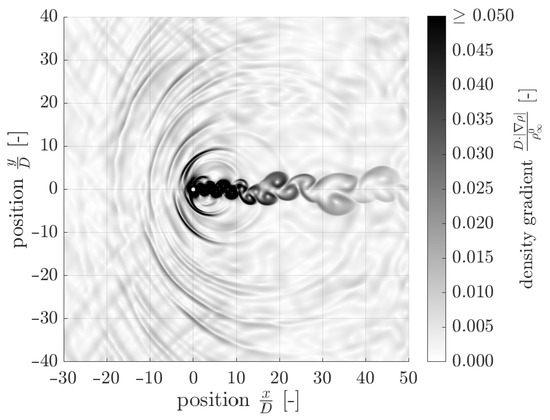
Figure 25. $R{e}_D=$ 13,300 and $M{a}_{\infty }=0.6$, distribution of $\frac{D·\left|\nabla \rho \right|}{{\rho }_{\infty }^0}$.

6. Conclusions

The applicability of the commercially available tool Ansys CFX was verified and validated. The distribution of the Mach number $Ma$ along a planar Laval nozzle showed that there are about eight to nine cells necessary to resolve a shock wave in comparison to the abrupt transition over a few mean free paths of the molecules. For validation, the Strouhal number $Str$ and the drag coefficient ${\overline{C}}_{\mathrm{D}}$ at $M{a}_{\infty }=0.2$ and 2 at $R{e}_D=100$ are compared to Burbeau and Sagaut [17] and they are in good agreement with a maximum deviation of 4%. In addition, even the detached shock wave position and the flow phenomena at the conditions investigated agree well with Burbeau and Sagaut [17]. Moreover, the validation showed that a higher-order advection scheme is necessary for adequate prediction of periodic vortex shedding and shock waves. Eight flow regimes were found in the planar flow around a circular cylinder for $50\le R{e}_D\le 300$ and 8890 $\le R{e}_D\le$ 80,000 and $0.2\le M{a}_{\infty }\le 2$. The modulus of the dimensionless density gradient $\frac{D·\left|\nabla \rho \right|}{{\rho }_{\infty }^0}$ has proven to be suitable for identifying and distinguishing between different flow phenomena, such as vortices, shocks, tangential discontinuities and sound waves. The simulation results at low $M{a}_{\infty }$ are found to be in similar flow regimes compared to the incompressible flow. At higher velocity near the speed of sound a, shocks occur. The cylinder wake in the turbulent regime behaves in a steady state and symmetrically and for $50\le R{e}_D\le 300$ vortices are formed in the cylinder wake. For some conditions in the transonic regime, for example $R{e}_D=300$ and $M{a}_{\infty }=0.5$, sound wave propagation occurs. The sound waves were identified by retracing the free-stream Mach number $M{a}_{\infty }$ from circles, which are fitted through the sound waves. Furthermore, the critical Mach number $M{a}_{\mathrm{crit}}$, the lowest $M{a}_{\infty }$ where the flow around the cylinder reaches the speed of sound, decreases with increasing Reynolds number $R{e}_D$ and for $R{e}_D\to \infty$ it is $M{a}_{\mathrm{crit}}=0.4$ from 38. The $C_{\mathrm{D}}$-$C_{\mathrm{L}}$-diagram shows a close curve in cases of laminar vortex shedding, but not for turbulent vortex shedding. A close curve corresponds to a given frequency ratio and a given phase shift of $C_{\mathrm{D}}$ and $C_{\mathrm{L}}$.

References

- Schlichting, H.; Gersten, K. Boundary-Layer Theory, 9th ed.; Springer: Berlin/Heidelberg, Germany, 2017. [Google Scholar] [CrossRef]
- Macha, J.M. Drag of circular cylinders at transonic Mach numbers. J. Aircr. 1977, 14, 605–607. [Google Scholar] [CrossRef]
- Murthy, V.; Rose, W. Form drag, skin friction and vortex shedding frequencies for subsonic and transonic crossflows on circular cylinder. In Proceedings of the 10th Fluid and Plasmadynamics Conference, Albuquerque, NM, USA, 27–29 June 1977; p. 687. [Google Scholar] [CrossRef]
- Rodriguez, O. The circular cylinder in subsonic and transonic flow. AIAA J. 1984, 22, 1713–1718. [Google Scholar] [CrossRef]
- Ackerman, J.; Gostelow, J.; Rona, A.; Carscallen, W.E. Base Pressure Measurements on a Circular Cylinder in Subsonic Cross Flow. In Proceedings of the 38th Fluid Dynamics Conference and Exhibit, Seattle, WA, USA, 23–26 June 2008; p. 4305. [Google Scholar] [CrossRef]
- Nagata, T.; Noguchi, A.; Kusama, K.; Nonomura, T.; Komuro, A.; Ando, A.; Asai, K. Experimental investigation on compressible flow over a circular cylinder at Reynolds number of between 1000 and 5000. J. Fluid Mech. 2020, 893, A13. [Google Scholar] [CrossRef]
- Gowen, F.E.; Perkins, E.W. Drag of circular cylinders for a wide range of Reynolds numbers and Mach numbers. NACA TN 1953, 2960. [Google Scholar]
- Botta, N. The inviscid transonic flow about a cylinder. J. Fluid Mech. 1995, 301, 225–250. [Google Scholar] [CrossRef]
- Bobenrieth Miserda, R.F.; Leal, R.G. Numerical Simulation of the Unsteady Aerodynamic Forces over a Circular Cylinder in Transonic Flow. In Proceedings of the 44th AIAA Aerospace Sciences Meeting and Exhibit, Reno Hilton, NV, USA, 9–12 January 2006; p. 1408. [Google Scholar] [CrossRef]
- Xu, C.Y.; Chen, L.W.; Lu, X.Y. Effect of Mach number on transonic flow past a circular cylinder. Chin. Sci. Bull. 2009, 54, 1886–1893. [Google Scholar] [CrossRef]
- Hong, R.; Xia, Z.; Shi, Y.; Xiao, Z.; Chen, S. Constrained large-eddy simulation of compressible flow past a circular cylinder. Commun. Comput. Phys. 2014, 15, 388–421. [Google Scholar] [CrossRef]
- Canuto, D.; Taira, K. Two-dimensional compressible viscous flow around a circular cylinder. J. Fluid Mech. 2015, 785, 349–371. [Google Scholar] [CrossRef]
- Xia, Z.; Xiao, Z.; Shi, Y.; Chen, S. Mach number effect of compressible flow around a circular cylinder. AIAA J. 2016, 54, 2004–2009. [Google Scholar] [CrossRef]
- Shirani, E. Compressible Flow Around A Circular Cylinder. Pak. J. Appl. Sci. 2001, 1, 472–476. [Google Scholar] [CrossRef]
- Matar, C.; Cinnella, P.; Gloerfelt, X.; Sundermeier, S.; Hake, L.; aus der Wiesche, S. Numerical investigation of the transonic non-ideal gas flow around a circular cylinder at high Reynolds number. In Proceedings of the Workshop Direct and Large-Eddy Simulation (DLES13), Udine, Italy, 26–29 October 2022. [Google Scholar]
- Linn, R.V.; Awruch, A.M. Adaptative finite element simulation of unsteady turbulent compressible flows on unstructured meshes. Comput. Fluids 2023, 254, 105816. [Google Scholar] [CrossRef]
- Burbeau, A.; Sagaut, P. Simulation of a viscous compressible flow past a circular cylinder with high-order discontinuous Galerkin methods. Comput. Fluids 2002, 31, 867–889. [Google Scholar] [CrossRef]
- Barth, T.J.; Jesperson, D.C. The Design and Application of Upwind Schemes on Unstructured Meshes. AIAA Pap. 1989, 27, 366. [Google Scholar] [CrossRef]
- Rhie, c.M.; Chow, W.L. A Numerical Study of the Turbulent Flow Past an Isolated Airfoil with Trailing Edge Separation. AIAA Pap. 1982, 21, 1525–1532. [Google Scholar] [CrossRef]
- Majumdar, S. Role of Underrelaxation in Momentum Interpolation for Calculation of Flow with Nonstaggered Grids. Numer. Heat Transf. 1988, 13, 125–132. [Google Scholar] [CrossRef]
- Menter, F.R. Zonal Two Equation k − ω Turbulence Models for Aerodynamic Flows. AIAA J. 1994, 32, 1598–1605. [Google Scholar] [CrossRef]
- Ansys Inc. and Ansys Europe. Ansys CFX-Solver Modeling Guide; Ansys Inc. and Ansys Europe: Canonsburg, PA, USA, 2022. [Google Scholar]
- Braza, M.; Chassaing, P.H.H.M.; Minh, H.H. Numerical study and physical analysis of the pressure and velocity fields in the near wake of a circular cylinder. J. Fluid Mech. 1986, 165, 79–130. [Google Scholar] [CrossRef]
- Ansys Inc. Ansys Documentation; Ansys Inc.: Canonsburg, PA, USA, 2022. [Google Scholar]
- Ansys Inc. GroupoSSC. 2014. Available online: https://www.grupossc.com/ponencias/ponencia_39114164442.pdf (accessed on 8 July 2020).
- Ansys Inc. Ansys Customer Portal. 2010. Available online: https://support.ansys.com/staticassets/ANSYS%20UK/staticassets/Reliable%20and20Accurate%20CFD%20Solutions,%20Mark%20Keating.pdf (accessed on 8 July 2020).
- Lesaint, P.; Raviart, P.A. On a Finite Element Method to Solve the Neutron Transport Equation; Partial Differentiel Equations. C. de Boor; Academic Press: New York, NY, USA, 1974. [Google Scholar] [CrossRef]
- Oden Tinsley, J.; Babuŝka, I.; Baumann, C.E. A discontinuoushpfinite element method for diffusion problems. J. Comput. Phys. 1998, 146, 491–519. [Google Scholar] [CrossRef]
- Van Dyke, M. An Album of Fluid Motion; Parabolic Press Stanford: Stanford, CA, USA, 1982. [Google Scholar]
- Müller, B. Towards high order numerical simulation of aeolian tones. PAMM 2005, 5, 473–474. [Google Scholar] [CrossRef]
- Khalili, M.E.; Larsson, M.; Müller, B. High-order ghost-point immersed boundary method for viscous compressible flows based on summation-by-parts operators. Int. J. Numer. Methods Fluids 2019, 89, 256–282. [Google Scholar] [CrossRef]
- Seo, J.H.; Moon, Y.J. Perturbed compressible equations for aeroacoustic noise prediction at low mach numbers. AIAA J. 2005, 43, 1716–1724. [Google Scholar] [CrossRef]
- Tsutahara, M.; Kataoka, T.; Shikata, K.; Takada, N. New model and scheme for compressible fluids of the finite difference lattice Boltzmann method and direct simulations of aerodynamic sound. Comput. Fluids 2008, 37, 79–89. [Google Scholar] [CrossRef]
- Cheong, C.; Joseph, P.; Park, Y.; Lee, S. Computation of aeolian tone from a circular cylinder using source models. Appl. Acoust. 2008, 69, 110–126. [Google Scholar] [CrossRef]
- Dumbser, M. Arbitrary high order PNPM schemes on unstructured meshes for the compressible Navier–Stokes equations. Comput. Fluids 2010, 39, 60–76. [Google Scholar] [CrossRef]
- de Tullio, M.D.; De Palma, P.; Iaccarino, G.; Pascazio, G.; Napolitano, M. Immersed boundary technique for compressible flow simulations on semi-structured grids. In Compitational Fluid Dynamics 2006, Proceedings of the Fourth International Conference on Computational Fluid Dynamics, ICCFD; Ghent, Belgium, 10–14 July 2006, Springer: Berlin/Heidelberg, Germany, 2009; pp. 365–370. [Google Scholar] [CrossRef]
- Hinman, S.W.; Johansen, C.T.; Arisman, C.J.; Galuppo, W.C. Numerical investigation of laminar near wake separation on circular cylinders at supersonic velocities. In Proceedings of the Congress of the International Council of the Aeronautical Sciences, St. Petersburg, Russia, 7–12 September 2014. [Google Scholar]
- Polhamus, E.C. A review of some Reynolds number effects related to bodies at high angles of attack. NASA Contract. Rep. 1984, 3809. [Google Scholar]
Disclaimer/Publisher’s Note: The statements, opinions and data contained in all publications are solely those of the individual author(s) and contributor(s) and not of MDPI and/or the editor(s). MDPI and/or the editor(s) disclaim responsibility for any injury to people or property resulting from any ideas, methods, instructions or products referred to in the content. |
© 2023 by the authors. Licensee MDPI, Basel, Switzerland. This article is an open access article distributed under the terms and conditions of the Creative Commons Attribution (CC BY) license (https://creativecommons.org/licenses/by/4.0/).