Air Flow Monitoring in a Bubble Column Using Ultrasonic Spectrometry

Abstract

This work demonstrates the use of an ultrasonic methodology to monitor bubble density in a water column. A flow regime with droplet size distribution between 0.2 and 2 mm was studied. This range is of particular interest because it frequently appears in industrial flows. Ultrasound is typically used when the size of the bubbles is much larger than the wavelength (low frequency limit). In this study, the radius of the bubbles ranges between 0.6 and 6.8 times the wavelength, where wave propagation becomes a complex phenomenon, making existing analytical methods difficult to apply. Measurements in transmission–reception mode with ultrasonic transducers operating at frequencies of 2.25 and 5.0 MHz were carried out for different superficial velocities. The results showed that a time-averaging scheme is necessary and that wave parameters such as propagation velocity and the slope of the phase spectrum are related to the number of bubbles in the column. The proposed methodology has the potential for application in industrial environments.

1. Introduction

Bubbly flows are integral to a variety of industrial operations, including alloy production, two-phase heat exchangers, reactor aeration and agitation, flotation equipment, and bubble column reactors. Bubble columns, where numerous gas bubbles travel upward through a liquid, are commonly utilized in the chemical, petrochemical, and biotechnological industries. These reactors play a crucial role in chemical processes like Fischer–Tropsch synthesis, fine chemical manufacturing, oxidation reactions, coal liquefaction, and fermentation [1]. Bubble column reactors are favored due to their simple construction and the absence of mechanically moving parts, which facilitates easy maintenance and lowers operating costs. Additionally, these reactors offer large interfacial areas and high transport rates, resulting in superior heat and mass transfer efficiency. This makes them highly effective for processes requiring significant interaction between gas and liquid phases [2].

In a bubble column, there are two different flow regimes depending on the superficial gas velocity U (the volumetric flow of air divided by the cross-sectional area of the column). By increasing U, an increase in the gas holdup $\epsilon$ (the number of bubbles per unit of volume) is observed. At the beginning, this increase is almost proportional and the homogeneous bubbly flow regime occurs, where the distribution of bubble sizes is narrow (1–7 mm) and the gas rise velocity is low, although trajectories of individual bubbles experience non-linear instabilities [3]. Above a transition superficial gas velocity, the coalescence phenomenon becomes important and large bubbles form and rise at a higher velocity. In this case, a heterogeneous or churn-turbulent flow regime occurs, with small bubbles that coexist with much larger ones (20–70 mm), and important horizontal velocity components are present, generating the mixing of the liquid phase [4,5]. When the gas in a vertical pipe occupies almost the entire cross section, this bullet-shaped bubble is called a Taylor bubble [6].

In a homogeneous bubbly flow, the individual bubbles move through the continuous liquid phase at low liquid superficial velocities and the interaction between them is negligible [7]. These kind of flows are found in boiling water nuclear reactors, steam generators, and refrigeration and air conditioning equipment [8]. On the other hand, the addition of bubbles in some industrial processes has been shown to be beneficial, for example, by increasing the efficiency of mixing or heat transfer between fluids, and the reaction rate in chemical reactors [9]. Therefore, the characterization or monitoring of these flows is important for the chemical, pharmaceutical, nuclear, and petrochemical industries. Another important area is environmental sciences, where the measurement of greenhouse gases migrating from the seafloor is an important topic [10].

For the characterization or monitoring of bubbly flows optical, electrical, and acoustical techniques have been used. In the case of optics, laser scattering [11] and laser-induced fluorescence [12] allow the density and relative size of the bubbles to be inferred. The passage of bubbles at a position in the column can be determined using an optical fiber immersed in the liquid [13], and this frequency can be related to the density of bubbles in the column. The pulse-light velocimetry (PLV) technique allows more precise measurement of bubble size and velocity [14], but the implementation of this technique requires expensive equipment and laboratory conditions. On the other hand, a relatively cheap and easy-to-implement technique is based on the digital processing of images captured with high-speed cameras. Edge detection algorithms are used to calculate the bubble density [15]. Overlapping, grouping, and irregular shapes of the bubbles are problems that are not easy to solve. To obtain accurate values, more than one camera and elaborate processing algorithms are needed [16,17]. However, the main disadvantage of optical methods is the opaqueness of many flows of interest. In this case, the use of x-rays has allowed the characterization of multi-phase flows [18]. But the measurement process can be complicated, requiring the capture and analysis of several planes or prior knowledge of some flow parameters. Furthermore, X-rays are a form of ionizing radiation that is harmful to life.

In the electrical case, measurements of the electric impedance in pairs of electrodes and the conductance in wire meshes are the main sensing approaches. The measurement of electrical impedance through a set of electrodes in contact with the medium under study is a cheap and relatively easy-to-implement technique that has gained attention in recent years [19]. Works related to the characterization of the stratified bubble flows and the study of the cavitation phenomenon are interesting examples [20]. These works use a single pair of electrodes, or a small number of them, to determine the electrical impedance at a certain frequency or range of working frequencies. The electrical impedance data can be related to the physical properties of the medium, and the flow dynamics can be analyzed using the temporal signal obtained. When a large number of electrodes are used, an image can be generated by solving an inverse problem. This technique is called electrical impedance tomography and it has been used to characterize multiphase flows [21,22,23]. In the case of wire-mesh tomography, the electrodes are wires arranged in a mesh pattern. Each crossing point of the wires serves as a sensing point [24]. In this case, the measurement is direct, and therefore, no reconstruction algorithms are needed. The resolution depends on the number of wires, and the data processing is fast, allowing for the measurement of hundreds of frames per second [25]. Although the electrical technique has much potential, its main disadvantage is that small chemical changes in the medium and material deposits on the electrodes or wires can affect the measurement.

Acoustical techniques use ultrasonic waves to infer the physical properties of the medium. Their main advantages are their capability to penetrate opaque media where optical techniques are not useful, the absence of ionizing radiation, and the fact that the required equipment is relatively simple and cheap [26]. In this respect, the ultrasonic characterization of heterogeneous media such as gas–liquid mixtures and immiscible liquids (emulsions) has been a topic of interest in recent years. Most of the works reported in the literature have been carried out with the limits of low frequency ($r/\lambda \ll 1$) and a low concentration of the dispersed phase [27,28,29]. Under these conditions, the propagation of ultrasonic waves is well behaved and there are analytical models that allow us to determine the droplet size spectrum from the ultrasonic signals. For example, these methods have been fundamental in the development and study of the contrast agents used in medical ultrasonography. These agents are fluids containing gas-filled microbubbles [30]. However, when the dispersed-phase droplets are of comparable ($r/\lambda \sim 1$) or larger ($r/\lambda \gg 1$) size than the wavelength, which is called the high-frequency limit, the propagation of ultrasonic waves becomes complicated. In these cases, there is an important interaction between the waves and the bubbles, generating large variations in the amplitude, and to a lesser extent in its phase, of the receiving waves. This behavior can be almost chaotic and the reception signal could even disappear.

Some works dealing with relatively large droplet sizes have been published in the literature. For instance, ultrasonic devices were developed to detect bubbles in the bloodstream [31]. The possibility of using common ultrasonic flow meters to determine the size of gas bubbles flowing through the pipe was evaluated, but it was only possible to obtain qualitative results [32]. The use of ultrasound and neural networks for the interpretation of data in the characterization of bubble flows in a water column was also reported. The bubble size was large ($r/\lambda \sim 65$) and a normalization scheme for the amplitude spectra [33] was used. Another work compared the analysis of ultrasound images obtained with a phased array and optical images for the characterization of a bubble flow, achieving similar results with both methods [10].

In this work, an ultrasonic methodology for bubble density monitoring in a water column is proposed. Measurements in transmission–reception mode and working frequencies of 2.25 and 5.0 MHz were carried out for different values of superficial gas velocity. Digital image processing allowed the characterization of the bubble flow, showing a droplet size distribution between 0.4 and 2.0 mm ($0.6\le r/\lambda \le 6.8$), almost independent of bubble density. By modifying the power supply voltage of the peristaltic pump it was possible to vary the amount of bubbles in the column. A signal-averaging scheme allowed us to circumvent the problem of large amplitude variations at reception. It was found that wave parameters such as the slope of the phase spectrum and the propagation velocity are closely related to the number of bubbles in the column, allowing the real-time monitoring of the bubbly flow. The proposed methodology is relatively simple and reliable, with potential for industrial application.

2. Materials and Methods

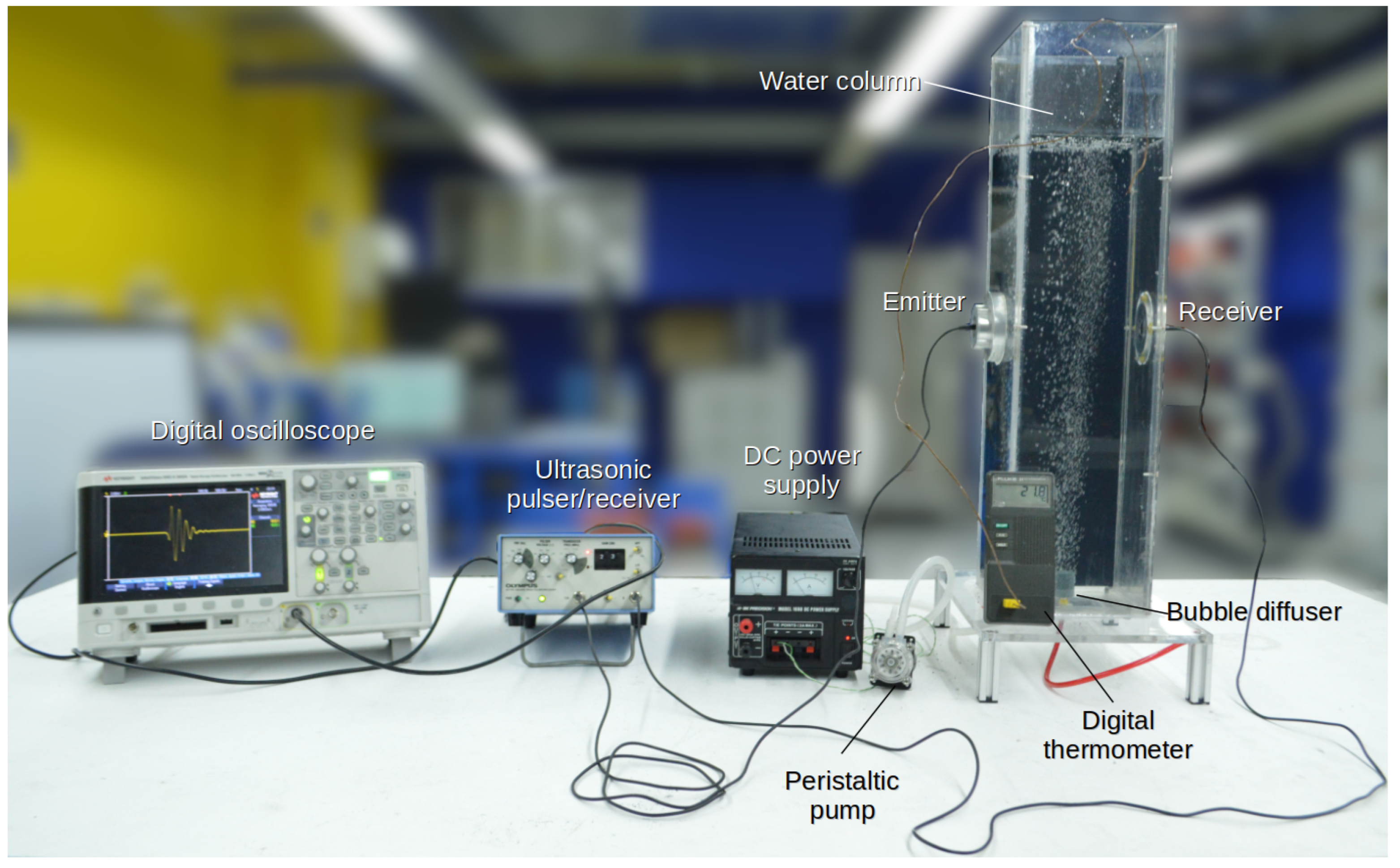
2.1. Experimental Setup

Figure 1 shows a scheme of the experimental setup, including the water column. The ultrasonic transducers were installed at half the height of the column, with metal brackets screwed to the acrylic wall to maintain alignment. The distance between the radiating surface of the transducers was approximately 151 mm. The column was filled with water to a level of approximately 160 mm above the transducers. A porous stone (diffuser) of the type used in decorative aquariums was installed at the bottom. The air was injected using a positive displacement pump (peristaltic pump) driven by a direct current (DC) motor powered by a laboratory power supply. The amount of bubbles in the column depended on the excitation voltage of the DC motor.

The transducers were driven by an ultrasonic pulse/receiver (Olympus 5077PR, Olympus NDT, Waltham, MA, USA), which excited the emitter with a high-voltage and short-duration pulse, and at the same time, amplified the signals that reached the receiver with gains of up to 40 dB. A digital oscilloscope with a bandwidth of 200 MHz (Keysight DSOX2022A, Keysight, Santa Rosa, CA, USA) synchronized with the pulser/receiver allowed the signals to be visualized and digitized. The ultrasonic signals were transferred to desktop computers through the LAN network and stored for later processing in Matlab (R2018b). All tests were carried out in a laboratory at room temperature, which was maintained at $23\pm 1.3$ °C by the air conditioning system. Temperature was measured using a digital thermometer with accuracy of $0.1$ °C. Figure 2 shows an image of the experimental setup, where all the components can be seen, except the desktop computer.

In this work, two pairs of ultrasonic transducers with a working frequency of 2.25 and 5.0 MHz from a well-known manufacturer (Krautkramer, Lewiston, PA, USA) were used.

Table 1. Main characteristics of the ultrasonic transducers used is this work.

Transducer	${\mathit{f}}_{\mathit{c}}$ (MHz)	$\mathit{\varphi }$ (mm)	BW ($-6$ dB)	${\mathit{Z}}_{\mathit{m}}$ (mm)	$\mathit{\theta }$ (degree)
Krautkrame 242–280	$2.25$	$12.7$	$32\%$	$61.3$	$3.62$
Krautkrame 254–360	$5.0$	24	$17\%$	486	$0.86$

reports the most relevant technical data, including the center frequency ($f_c$), the bandwidth (BW) of the signal acquired in water (without bubbles), calculated for a −6 dB amplitude drop, and the acoustic field parameters. These parameters are the near-field length, $Z_m={(\varphi /2)}^2/\lambda$, and the beam divergence angle, $sin(\theta /2)=1.22\lambda /\varphi$, where $\varphi$ is the diameter of the transducer radiating surface, $\lambda =c_w/f_c$ is the theoretical wavelength, and $c_w=1480$ m/s is the propagation velocity in water at $20$ °C. Figure 3 shows the waveform and the respective Fourier spectra of the ultrasonic pulses obtained in reception with water.

The excitation signal, as seen on the oscilloscope without the transducer connected, is a square pulse with an amplitude and a width that can be varied by certain set values. The width allows the pulse to be tuned to the transducer’s working frequency to achieve a better response. In the emission, we used an excitation pulse with an amplitude of 200 V, and gains between 0 and 10 dB were used in the receiver. Despite the high excitation voltage, the acoustic waves generated in pulse-echo mode are of low intensity. These are the waves used in ultrasonic non-destructive testing (UT-NDT), where other physical phenomena, such as cavitation or streaming, do not occur.

The transducer spacing is large compared to the wavelength, at $228\lambda$ and $508\lambda$ for the 2.25 and 5.0 MHz transducers, respectively. This allows clear reception of the ultrasonic pulses, without the problems of reverberation or spurious reflections. On the other hand, the diameter and frequency of the transducers cause the receiver to be located in the far field and the near field for the 2.25 and 5 MHz cases, respectively. This difference is not relevant due to the frequency domain normalization performed using the signal in the bubble-free case.

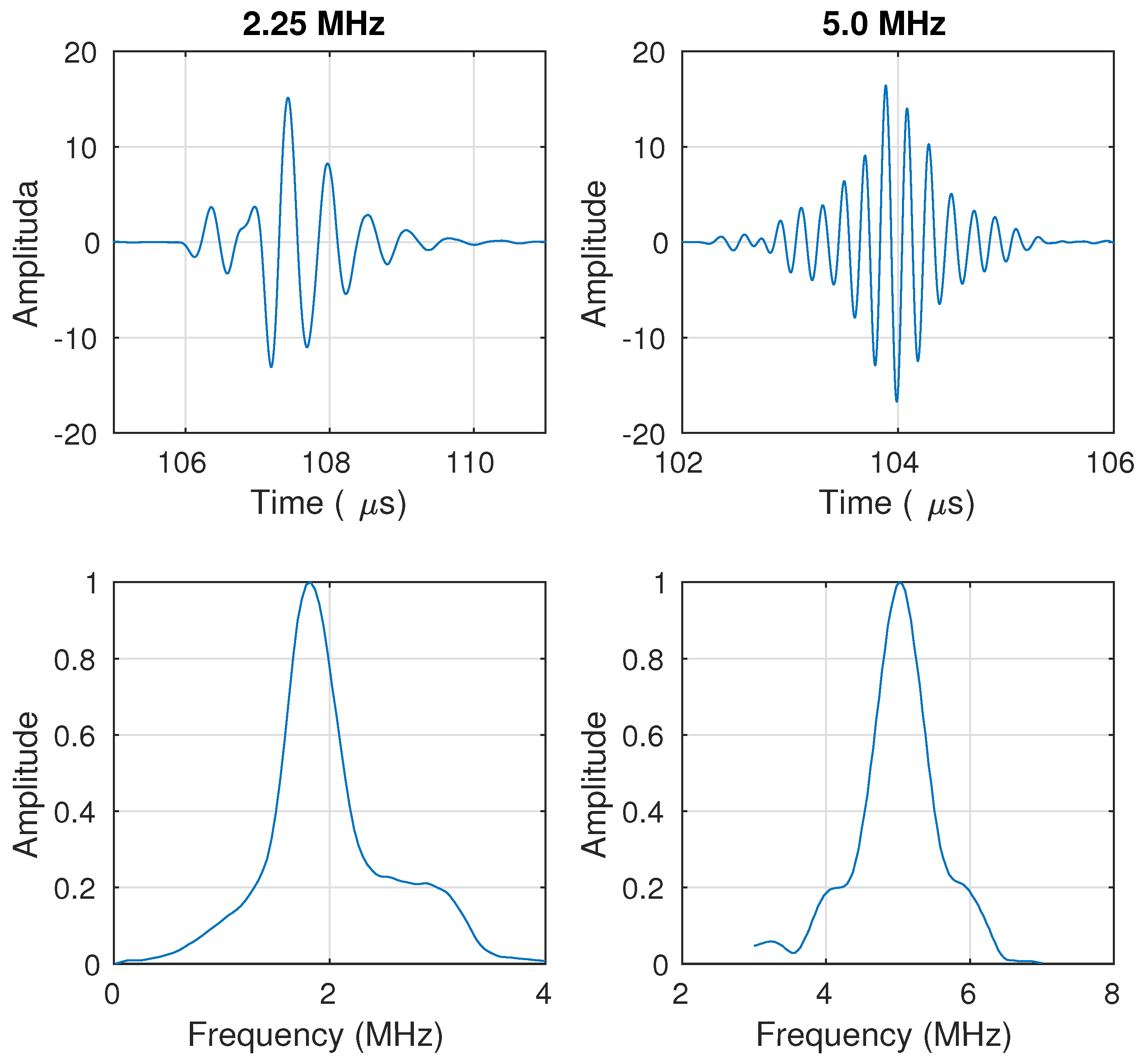
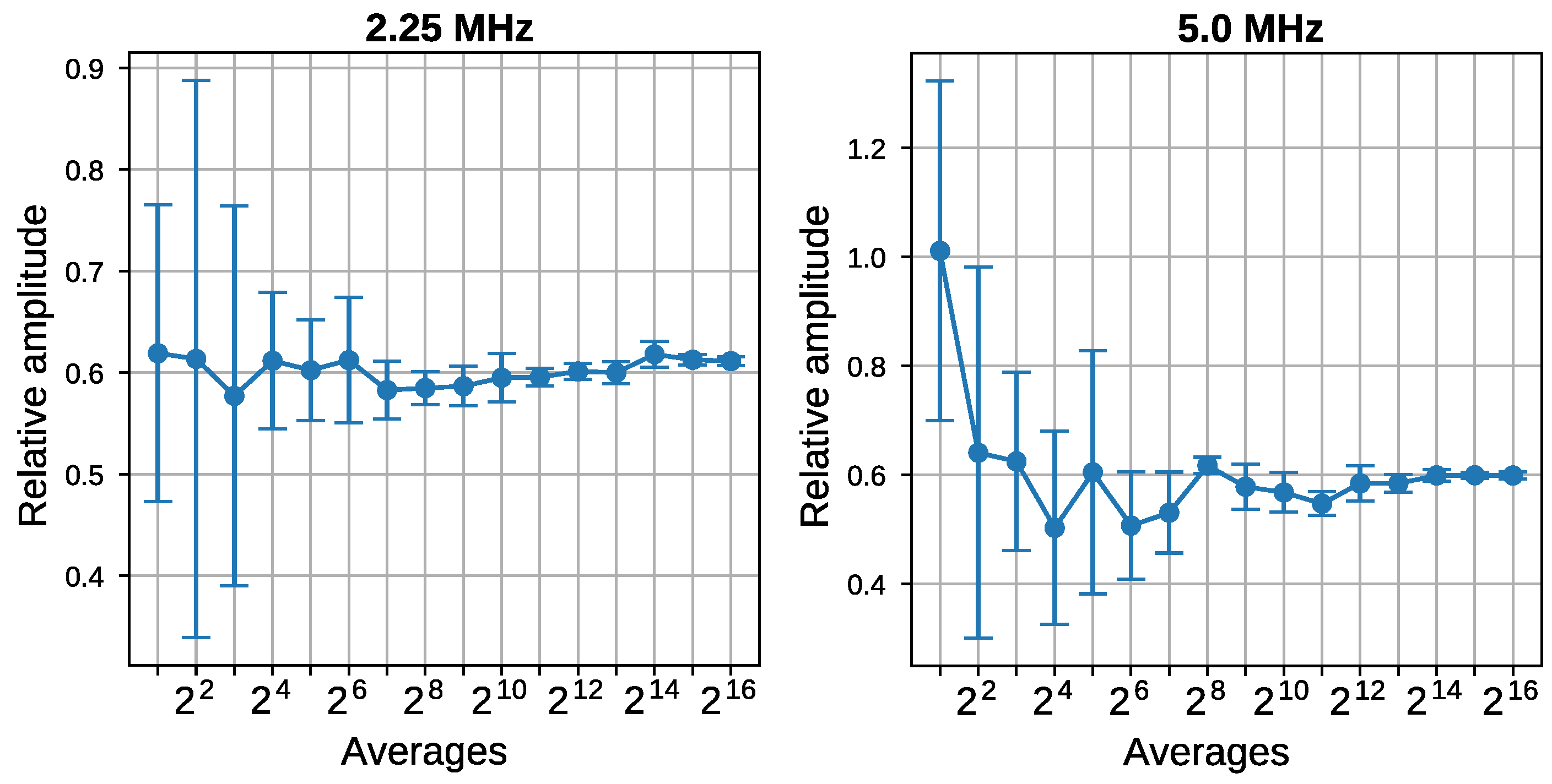
2.2. Signal Processing

Let $a_2\left(t\right)$ and $a_1\left(t\right)$ be the ultrasonic signals received in the cases with and without bubbles, respectively, where t is the time. In the case with bubbles, there is a drop in amplitude and a difference in the arrival time of the wave, which are related to diffraction, attenuation, and changes in the propagation velocity. The comparison between the cases with bubbles and the reference (without bubbles) is performed in the frequency domain using the loss coefficient (P):

$$P\left(f\right)=p{e}^{j\varphi },$$

(1)

where p and $\varphi$ are the magnitude and phase of the loss coefficient, which are calculated from the ultrasonic signals as follows:

$$p\left(f\right)={\displaystyle \frac{|A_2\left(f\right)|}{|A_1\left(f\right)|}}$$

(2)

and

$$\varphi =arg\left[A_2\left(f\right)\right]-arg\left[A_1\left(f\right)\right]$$

(3)

where $A_2\left(f\right)$ and $A_1\left(f\right)$ are the Fourier transforms of the signals $a_2\left(t\right)$ and $a_1\left(t\right)$, respectively, and f is the frequency.

The effect of the presence of bubbles on ultrasonic waves is analyzed by means of attenuation and phase spectra. The attenuation spectrum is given by [34]:

$$\alpha \left(f\right)={\displaystyle \frac{1}{d}}20log\left[p\left(f\right)\right]$$

(4)

where d is the distance between the face of the transducers (see Figure 1). The attenuation spectrum quantifies the amplitude reduction of each spectral component in a suitable frequency range around the center frequency of the transducer.

The velocity spectrum is obtained by calculating the additional time ($\delta$) that the wave takes, due to the presence of the bubbles, by means of the phase of the Fourier transform:

$$\delta ={\displaystyle \frac{\varphi }{2\pi }}T={\displaystyle \frac{\varphi }{2\pi f}}$$

(5)

where $T=1/f$ is the period. The velocity spectrum is calculated by dividing the distance traveled by the total time in the case with bubbles [34]:

$$v\left(f\right)={\displaystyle \frac{d}{{\delta }_0+\delta }}$$

(6)

where ${\delta }_0$ is the arrival time in the case without bubbles. Replacing ${\delta }_0$ and $\delta$ in (6), we obtain the expression for the velocity spectrum:

$$v\left(f\right)={\displaystyle \frac{d{v}_0\left(2\pi f\right)}{d\left(2\pi f\right)+v_0\varphi }},$$

(7)

where $v_0=d/{\delta }_0$ is the velocity in the reference case.

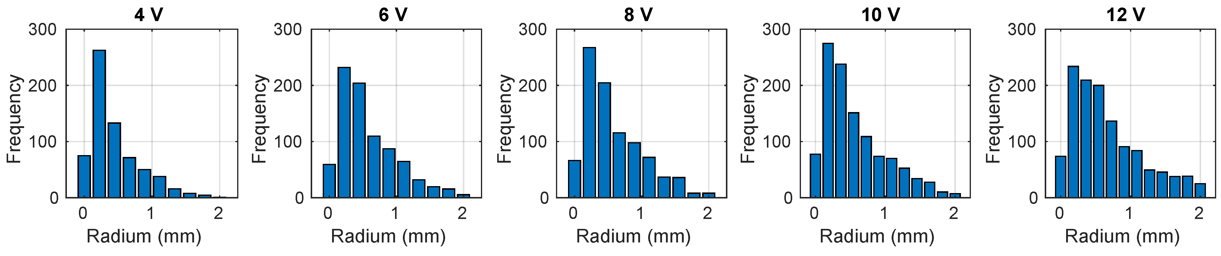
2.3. Characterization of the Bubble Column

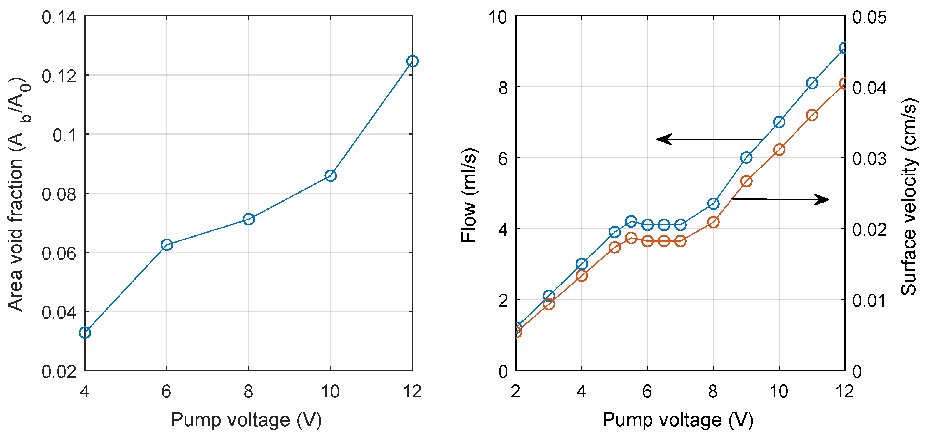
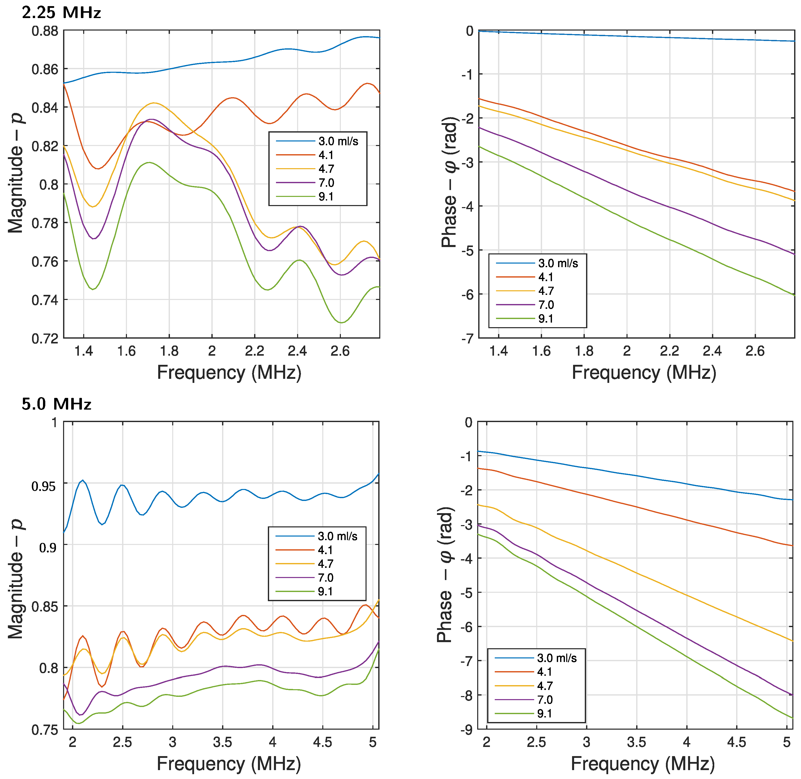
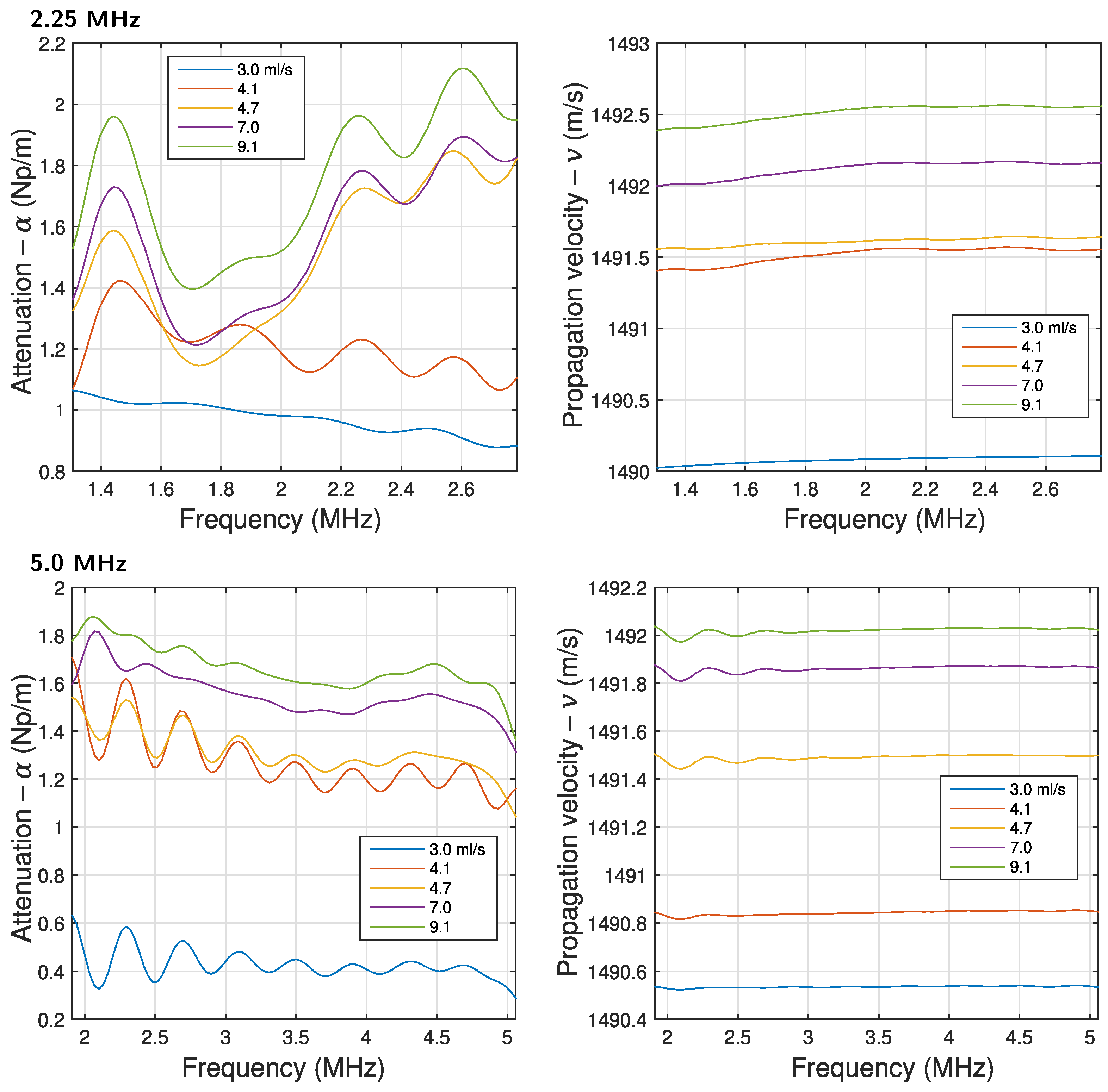
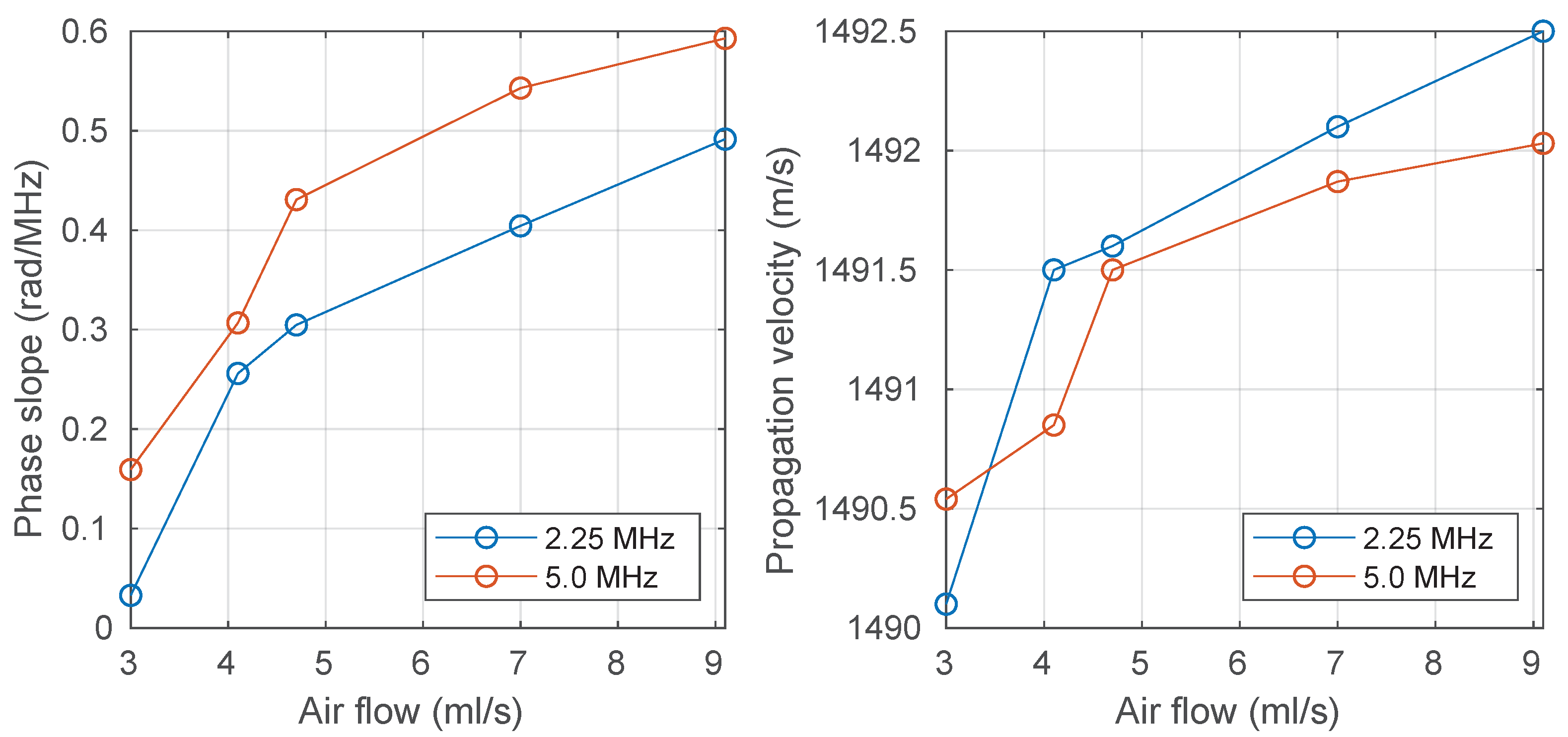
Figure 4 shows the image processing methodology used to estimate the bubble density. The images were captured with a reflex camera (Nikon D3200, Nikon, Tokyo, Japan) using a white background with a matte finish and high-intensity LED lighting. Due to the rise speed of the bubbles, a high shutter speed (1.25 ms) was necessary. First, a circular element was positioned on the axis that joins the center of the two ultrasonic transducers and a picture was taken. This circle of known diameter was a size reference for estimating the observed void area. Keeping the camera in the same position, pictures of the bubble column were taken. The air flow that generated the column of bubbles was controlled by the electrical voltage applied to the DC motor of the peristaltic pump.

To estimate the void fraction, a portion of the area observed by the camera was established. The transverse area illuminated by the surface transducer, including the divergence of the beam in the far field, was taken (see Figure 4 and Table 1). This area was defined with the intention of covering the area with the highest interaction between ultrasonic waves and bubbles. However, the results for both transducers were similar, and finally, only the area established with the larger-diameter transducer (5.0 MHz) was used.

The images with bubbles were analyzed using the $OpenCV$ Python library (https://opencv.org/ (accessed on 11 July 2024)). Processing began by converting each image to gray scale; then, segmentation and capture algorithms were applied. The processing was based on applying the Hough transform to detect circles [35]. The algorithm returned the coordinates of the centers and radii of the detected circles. Another algorithm was used to detect contours. The detected circles and contours are shown in red and green, respectively, in Figure 4 (bottom). The results of both algorithms presented similar values. However, contour detection presented more unexpected results, such as contours with areas of water inside, which required reprocessing or changing the image. The circle detection algorithm was more stable and probably more suitable for a possible practical application.

Figure 5 shows the histograms of the bubble size spectra for six excitation voltages of the peristaltic pump. The x-axis is the size range and the y-axis is the number of bubbles detected by the algorithm in each range. The results show that regardless of the excitation voltage, the highest count is within the 0.2 to 0.4 mm range. As the voltage is increased, the number of bubbles detected also increases, but it is the larger bubbles that show a more significant increase due to coalescence. The entire spectrum range remains almost the same (0–2 mm).

The area void fraction calculated by the image processing procedure is shown in Figure 6 (left). This value was calculated as the quotient between the sum of all the areas detected by the algorithm ($A_b$) and the area of influence of the acoustic beam ($A_0$) defined in Figure 4. These results show that the void fraction increases with the pump excitation voltage, as expected. This increase does not appear to be linear.

The peristaltic pump was also characterized to determine the volumetric flow (Q) as a function of the excitation voltage. In a test, the time required to pump a certain volume of liquid was measured. Figure 6 (right) shows the injected air flow and the superficial velocity as a function of the pump voltage. The shape of the curve is similar to that of the void fraction obtained by digital image processing. Clearly, there is a linear behavior in the 2–5 and 8–12 V ranges. Between 5.2 and 7 V, approximately, the flow remains constant. These results are important because they relate the wave parameters to the actual air flow. By dividing the air flow by the cross-sectional area of the column (225 cm²), the superficial velocity was obtained.

3. Results

The behavior of acoustic waves in reception is chaotic due to the relative size of the bubbles. For the analysis shown in this work, a diffuser (porous stone) that provides bubbles with an average radius of 400 μm and maximum radii close to 2 mm (see Figure 5) was used. These bubble sizes lead to values of $0.6<r/\lambda <3.0$ and $1.4<r/\lambda <6.8$ for the working frequencies for 2.25 and 5.0 MHz, respectively. Therefore, most bubbles are of similar size, and some others several times larger than the wavelength. In this measurement range, there is a high interaction of the ultrasonic waves with the bubbles, causing large variations in the amplitude observed in reception.

Figure 7 shows the mean and standard deviation of the loss coefficient as a function of the signal averages, calculated at the central frequency of each transducer. The results show how the mean value stabilizes and the standard deviation reduces dramatically as the averages increase. The mean value is very close to 0.6 for both frequencies. The repetition rate used in the ultrasonic pulser/receiver is 5 kHz. Therefore, the acquisition times are relatively short in spite of the high number of averages. For example, the acquisition times for the $2^{12}$ and $2^{16}$ averages are 0.82 and 13 s, respectively. These times are short enough to perform several measurements per minute. However, the transfer, storage, and processing time on the computer must be added, which, depending on the hardware, may be relevant.

Figure 8 shows the magnitude and phase of the loss coefficient as a function of frequency for the two transducers in a frequency band of −12 dB. The signals were acquired with ${10}^{15}$ averages and the temperature in the water column was $23.1$ °C. In the case of the magnitude of the loss coefficient, the results show a complicated spectrum, with oscillations and increasing and decreasing trends. For 2.25 MHz, the size of the bubbles is closer to the wavelength and there is greater interaction, with increasing magnitude values as the frequency increases. For 5.0 MHz, all magnitudes decrease with frequency. However, for both working frequencies, decreasing magnitude with a decreasing amount of bubbles can be observed. When the average value or the area under the curve was calculated, the results were erratic. In the case of the phase of the loss coefficient, a more stable and almost linear behavior was observed. This result is the expected in the case of a receiving ultrasonic pulse, and clearly, the slope of the phase is related to the amount of bubbles.

Figure 9 shows the attenuation and propagation velocity spectra in the −12 dB band for the two working frequencies. Since the attenuation spectrum depends on the magnitude of the loss coefficient, its behavior is very similar to that shown in Figure 8. On the other hand, the propagation velocity can be calculated at any frequency. In this case, the velocity was calculated at the central frequency of the transducer (see Figure 3). These results show an approximately constant propagation velocity as a function of frequency, which increases with the number of bubbles. The propagation velocity measured without bubbles was 1489.1 m/s at 23.1 °C, and the value reported in the literature is 1491.5 m/s [36,37]. Even though the velocity increase due to the presence of bubbles is only 2 m/s for for an air flow variation of 6.0 mL/s, which is equivalent to 0.13%, perfectly separated curves are observed for the air flow valuer. This shows that the system has good resolution and stability for measuring propagation velocity.

These results allow us to conclude that in this heterogeneous medium with bubbles, the phase is more stable and useful for bubble density monitoring than the magnitude. This becomes clearer when it is recalled that the phase is related to the arrival time of the waves, and the magnitude to the measured acoustic pressure. This result is in agreement with that reported by other authors who worked with homogeneous media and emulsions [38].

Figure 10 (left) shows the slope of the phase spectrum and the propagation velocity as a function of the air flow in the column for the two working frequencies. In the case of the phase slope, both curves show a monotonically rising tendency with the air flow, with less variation at 5 MHz. Considering that the slope of the phase spectrum is zero for the bubble-free case due to normalization, the range of variation is 0.5 and 0.6 rad/MHz for 2.25 and 5.0 MHz, respectively. The slope of the phase spectrum was already used for monitoring of the water content in water-in-crude oil emulsions [39]. In this case, the phase slope variation was higher, up to 12 rad/MHz. This difference must be a consequence of the concentration in both heterogeneous media. However, such a value is also affected by some measurement parameters, for example, the distance at which the waves interact with the bubbles of the dispersed phase.

In the case of propagation velocity shown in Figure 10 (right), a similar behavior with a clearly increasing trend is observed. The behavior seems less stable, with points further away from this trend. It can be seen that the total variation in propagation velocity is 2.5 m/s; such small variations (0.17%) must have a considerable error component due to random noise. In measurements carried out in water-in-crude oil emulsions with a volumetric concentration of up to 40%, variations in the propagation velocity of up to 30 m/s were observed [38]. In that case, it can be stated that the difference in propagation velocity is exclusively a consequence of the concentration of the dispersed phase in the media.

These results show the possibility of monitoring the amount of bubbles in the water column using both the slope of the phase spectrum and the propagation velocity. Both properties can be used to obtain calibration curves that directly provide the air flow or superficial velocity. However, the analysis of the influence of temperature and the applicability of the technique with higher concentrations requires further research.

4. Conclusions

This work proposes a simple and inexpensive methodology based on ultrasonic spectrometry for monitoring the bubble density in a water column. Tests were carried out at two working frequencies in transmission–reception mode for different values of superficial velocity. The amount of bubbles was determined by characterizing the positive displacement pump used for air injection. On the other hand, digital image analysis allowed us to establish the droplet size spectrum, showing bubble radii comparable to or greater than the wavelength. Under these conditions, wave propagation is complicated, with large variations in amplitude, even leading to signal disappearance at reception. To overcome this problem, a signal averaging scheme proved to be an appropriate strategy.

Signal analysis was performed in the frequency domain using a loss coefficient, and attenuation and velocity spectra. The results were normalized using a reference case without bubbles. The amplitude of the loss coefficient and the attenuation spectrum showed an intricate behavior that could not be related to the number of bubbles. On the other hand, the phase of the loss coefficient and the velocity spectrum showed a more stable behavior, dependent on the number of bubbles. The best case was provided by the slope of the phase spectrum, which displays monotonic growth with the superficial velocity.

Our results showed the possibility of monitoring the density of bubbles in the water column using the phase spectrum of the loss coefficient. The proposed methodology is relatively simple and inexpensive, and the signal processing requires little computational power, making it possible to use low-cost microcontrollers. The studied regime, with the presence of large droplets compared to the wavelength, is interesting because it occurs in important industrial processes, for instance, in chemical reactors, with little information in the literature about non-destructive testing by ultrasound.

Finally, the main limitations of the proposed technique are its applicability at high temperatures and concentrations. This technique will probably require a calibration process for each working temperature. Additionally, at temperatures above 100 °C, conventional ultrasonic transducers may present problems, such as large temperature gradients that affect their operation or even permanent depolarization of the piezoelectric material. On the other hand, with concentrations higher than those used in this work, the signals must have a more complex behavior, and the proposed methodology will probably not be applicable. For these cases, additional research is required.

References

1. Sokolichin, A.; Eigenberger, G.; Lapin, A. Simulation of buoyancy driven bubbly flow: Established simplifications and open questions. AIChE J. 2004, 50, 24–45. [Google Scholar] [CrossRef]
2. Lain, S.; Bröder, D.; Sommerfeld, M. Experimental and numerical studies of the hydrodynamics in a bubble column. Chem. Eng. Sci. 1999, 54, 4913–4920. [Google Scholar] [CrossRef]
3. Göz, M.; Laín, S.; Sommerfeld, M. Study of the numerical instabilities in Lagrangian tracking of bubbles and particles in two-phase flow. Comput. Chem. Eng. 2004, 28, 2727–2733. [Google Scholar] [CrossRef]
4. Krishna, R.; van Baten, J. Mass transfer in bubble columns. Catal. Today 2003, 79–80, 67–75. [Google Scholar] [CrossRef]
5. Laín, S.; Bröder, D.; Sommerfeld, M.; Göz, M. Modelling hydrodynamics and turbulence in a bubble column using the Euler–Lagrange procedure. Int. J. Multiph. Flow 2002, 28, 1381–1407. [Google Scholar] [CrossRef]
6. Ambrose, S.; Hargreaves, D.M.; Lowndes, I.S. Numerical modeling of oscillating Taylor bubbles. Eng. Appl. Comput. Fluid Mech. 2016, 10, 578–598. [Google Scholar] [CrossRef]
7. Etminan, A.; Muzychka, Y.S.; Pope, K. A Review on the Hydrodynamics of Taylor Flow in Microchannels: Experimental and Computational Studies. Processes 2021, 9, 870. [Google Scholar] [CrossRef]
8. Asiagbe, K.S.; Fairweather, M.; Njobuenwu, D.O.; Colombo, M. Large Eddy Simulation of Microbubble Transport in Vertical Channel Flows. In Computer Aided Chemical Engineering; Espuña, A., Graells, M., Puigjaner, L., Eds.; Elsevier: Amsterdam, The Netherlands, 2017; Volume 40, pp. 73–78. [Google Scholar] [CrossRef]
9. Dabiri, S.; Tryggvason, G. Heat transfer in turbulent bubbly flow in vertical channels. Chem. Eng. Sci. 2015, 122, 106–113. [Google Scholar] [CrossRef]
10. Takimoto, R.Y.; Matuda, M.Y.; Oliveira, T.F.; Adamowski, J.C.; Sato, A.K.; Martins, T.C.; Tsuzuki, M.S. Comparison of Optical and Ultrasonic Methods for Quantification of Underwater Gas Leaks. IFAC-PapersOnLine 2020, 53, 16721–16726. [Google Scholar] [CrossRef]
11. Abbaszadeh, M.; Alishahi, M.M.; Emdad, H. A new bubbly flow detection and quantification procedure based on optical laser-beam scattering behavior. Meas. Sci. Technol. 2020, 32, 025202. [Google Scholar] [CrossRef]
12. Alméras, E.; Cazin, S.; Roig, V.; Risso, F.; Augier, F.; Plais, C. Time-resolved measurement of concentration fluctuations in a confined bubbly flow by LIF. Int. J. Multiph. Flow 2016, 83, 153–161. [Google Scholar] [CrossRef]
13. Ma, Y.; Muilwijk, C.; Yan, Y.; Zhang, X.; Li, H.; Xie, T.; Qin, Z.; Sun, W.; Lewis, E. Measurement of Bubble Flow Frequency in Chemical Processes Using an Optical Fiber Sensor. In Proceedings of the 2018 IEEE SENSORS, New Delhi, India, 28–31 October 2018; pp. 1–4. [Google Scholar] [CrossRef]
14. Bröder, D.; Sommerfeld, M. Planar shadow image velocimetry for the analysis of the hydrodynamics in bubbly flows. Meas. Sci. Technol. 2007, 18, 2513. [Google Scholar] [CrossRef]
15. Shamoun, B.; Beshbeeshy, M.E.; Bonazza, R. Light extinction technique for void fraction measurements in bubbly flow. Exp. Fluids 1999, 26, 16–26. [Google Scholar] [CrossRef]
16. Fu, Y.; Liu, Y. Development of a robust image processing technique for bubbly flow measurement in a narrow rectangular channel. Int. J. Multiph. Flow 2016, 84, 217–228. [Google Scholar] [CrossRef]
17. Karn, A.; Ellis, C.; Arndt, R.; Hong, J. An integrative image measurement technique for dense bubbly flows with a wide size distribution. Chem. Eng. Sci. 2015, 122, 240–249. [Google Scholar] [CrossRef]
18. Lau, Y.; Möller, F.; Hampel, U.; Schubert, M. Ultrafast X-ray tomographic imaging of multiphase flow in bubble columns—Part 2: Characterisation of bubbles in the dense regime. Int. J. Multiph. Flow 2018, 104, 272–285. [Google Scholar] [CrossRef]
19. Cabrera-López, J.J.; Velasco-Medina, J. Structured Approach and Impedance Spectroscopy Microsystem for Fractional-Order Electrical Characterization of Vegetable Tissues. IEEE Trans. Instrum. Meas. 2020, 69, 469–478. [Google Scholar] [CrossRef]
20. George, D.L.; Iyer, C.O.; Ceccio, S.L. Measurement of the Bubbly Flow Beneath Partial Attached Cavities Using Electrical Impedance Probes. J. Fluids Eng. 1999, 122, 151–155. [Google Scholar] [CrossRef]
21. Huang, C.; Lee, J.; Schultz, W.W.; Ceccio, S.L. Singularity image method for electrical impedance tomography of bubbly flows. Inverse Probl. 2003, 19, 919. [Google Scholar] [CrossRef]
22. de Moura, B.F.; Martins, M.F.; Palma, F.H.S.; da Silva, W.B.; Cabello, J.A.; Ramos, R. Nonstationary bubble shape determination in Electrical Impedance Tomography combining Gauss–Newton Optimization with particle filter. Measurement 2021, 186, 110216. [Google Scholar] [CrossRef]
23. Zhu, Z.; Li, G.; Luo, M.; Zhang, P.; Gao, Z. Electrical Impedance Tomography of Industrial Two-Phase Flow Based on Radial Basis Function Neural Network Optimized by the Artificial Bee Colony Algorithm. Sensors 2023, 23, 7645. [Google Scholar] [CrossRef] [PubMed]
24. Prasser, H.M.; Böttger, A.; Zschau, J. A new electrode-mesh tomograph for gas–liquid flows. Flow Meas. Instrum. 1998, 9, 111–119. [Google Scholar] [CrossRef]
25. Hampel, U.; Babout, L.; Banasiak, R.; Schleicher, E.; Soleimani, M.; Wondrak, T.; Vauhkonen, M.; Lähivaara, T.; Tan, C.; Hoyle, B.; et al. A Review on Fast Tomographic Imaging Techniques and Their Potential Application in Industrial Process Control. Sensors 2022, 22, 2309. [Google Scholar] [CrossRef] [PubMed]
26. Durán, A.L.; Franco, E.E.; Reyna, C.A.B.; Pérez, N.; Tsuzuki, M.S.G.; Buiochi, F. Water Content Monitoring in Water-in-Crude-Oil Emulsions Using an Ultrasonic Multiple-Backscattering Sensor. Sensors 2021, 21, 5088. [Google Scholar] [CrossRef] [PubMed]
27. Allegra, J.R.; Hawley, S.A. Attenuation of Sound in Suspensions and Emulsions: Theory and Experiments. J. Acoust. Soc. Am. 1972, 51, 1545–1564. [Google Scholar] [CrossRef]
28. Wu, X.; Chahine, G.L. Development of an acoustic instrument for bubble size distribution measurement. J. Hydrodyn. Ser. B 2010, 22, 330–336. [Google Scholar] [CrossRef]
29. Pinfield, V.J. Advances in ultrasonic monitoring of oil-in-water emulsions. Food Hydrocoll. 2014, 42, 48–55. [Google Scholar] [CrossRef]
30. de Jong, N.; Emmer, M.; van Wamel, A.; Versluis, M. Ultrasonic characterization of ultrasound contrast agents. Med. Biol. Eng. Comput. 2009, 47, 861–873. [Google Scholar] [CrossRef] [PubMed]
31. Kremkau, F.W.; Gramiak, R.; Carstensen, E.L.; Shah, P.M.; Kramer, D.H. Ultrasonic detection of cavitation at catheter tips. Am. J. Roentgenol. 1970, 110, 177–183. [Google Scholar] [CrossRef]
32. Nishi, R. Ultrasonic detection of bubbles with doppler flow transducers. Ultrasonics 1972, 10, 173–179. [Google Scholar] [CrossRef]
33. Baroni, D.B.; Filho, J.S.C.; Lamy, C.A.; Bittencourt, M.S.Q.; Pereira, C.M.N.A.; Motta, M.S. Determination of size distribution of bubbles in a ubbly column two-phase flows by ultrasound and neural networks. In Proceedings of the 2011 International Nuclear Atlantic Conference—INAC 2011, Brazzilian Asiciation of Nuclear Engineering—ABEN, Belo Horizonte, MG, Brazil, 24–28 October 2011. [Google Scholar]
34. Cents, A.H.G. Mass Transfer and Hydrodynamics in Stirred Gas-Liquid-Liquid Contactors. Ph.D. Thesis, Universiteit Twente, Enschede, The Netherlands, 2003. [Google Scholar]
35. Djekoune, A.O.; Messaoudi, K.; Amara, K. Incremental circle hough transform: An improved method for circle detection. Optik 2017, 133, 17–31. [Google Scholar] [CrossRef]
36. Lubbers, J.; Graaff, R. A simple and accurate formula for the sound velocity in water. Ultrasound Med. Biol. 1998, 24, 1065–1068. [Google Scholar] [CrossRef] [PubMed]
37. Del Grosso, V.A.; Mader, C.W. Speed of Sound in Pure Water. J. Acoust. Soc. Am. 1972, 52, 1442–1446. [Google Scholar] [CrossRef]
38. Reyna, C.A.; Franco, E.E.; Tsuzuki, M.S.; Buiochi, F. Water content monitoring in water-in-oil emulsions using a delay line cell. Ultrasonics 2023, 134, 107081. [Google Scholar] [CrossRef]
39. Franco, E.E.; Reyna, C.A.B.; Durán, A.L.; Buiochi, F. Ultrasonic Monitoring of the Water Content in Concentrated Water–Petroleum Emulsions Using the Slope of the Phase Spectrum. Sensors 2022, 22, 7236. [Google Scholar] [CrossRef]
Figure 1. Scheme of the experimental setup.
Fluids 09 00163 g001
Figure 2. Image of the experimental setup, including the water column including the two ultrasonic transducers.
Fluids 09 00163 g002
Figure 3. Waveforms and spectra of the ultrasonic transducers used in this work.
Fluids 09 00163 g003
Figure 4. Image processing methodology used for the bubble density estimation.
Fluids 09 00163 g004
Figure 5. Bar graph showing the bubble radius distribution obtained by image processing for five excitation voltages of the peristaltic pump.
Fluids 09 00163 g005
Figure 6. Area void fraction obtained with the image processing technique (left) and superficial gas velocity obtained in the characterization of the peristaltic pump (right).
Fluids 09 00163 g006
Figure 7. Mean and standard deviation of the loss coefficient as a function of the signal averages. p ( f ) were calculated at the central frequency of each transducer.
Fluids 09 00163 g007
Figure 8. Magnitude (p) and phase ( ϕ ) of the loss coefficient as a function of frequency for all the values of the air flow (frequency band of −12 dB, 10 15 averages, and test temperature of 23.1 °C).
Fluids 09 00163 g008
Figure 9. Attenuation ( α ) and velocity (v) spectra for all the values of the air flow (frequency band of −12 dB, 10 15 averages, and test temperature of 23.1 °C).
Fluids 09 00163 g009
Figure 10. Phase slope (left) and propagation velocity (right) as a function of the air flow in the column.
Fluids 09 00163 g010