Abstract
The earliest archaeological evidence of wine came from ceramic vessels of the Transcaucasian ‘Shulaveri-Shomutepe’ or ‘Aratashen-Shulaveri-Shomutepe culture’ (SSC/AShSh: c. 6000–5200 BC). Western European ‘Bell Beaker culture’ (BB: c. 2500–2000 BC) is characterized by bell-shaped pottery vessels but has so far not been found with residues consistent with wine. Knowing that wild grapes populated both habitats, the absence of wine during the Bell Beaker period remains to be explained. The main goal of this work was to investigate whether the shape of the vessels could influence the performance of spontaneous fermentation, specifically regarding the production of volatile acidity. Crushed grapes or juices from various grape cultivars were fermented in two types of vessels: (i) borosilicate glass beakers (4–5 L) to imitate bell beakers and (ii) Erlenmeyer flasks (5 L) to imitate SSC/AShSh vessels. Fermentations occurred spontaneously, and the wines were analyzed for their conventional physical–chemical parameters (e.g., ethanol content, total acidity, volatile acidity, pH), chromatic characteristics (e.g., wine color intensity, wine hue), and volatile composition by gas-chromatography-flame ionization detection (GC-FID). At the end of fermentation, the yeast species were identified by molecular methods. In addition, wine yields and phenolic composition (e.g., total phenols, anthocyanins, total pigments) were determined for wild grapes in comparison with six red varieties Vitis vinifera L. subsp. sativa (Vinhão, Marufo, Branjo, Melhorio, Castelão and Tempranillo Tinto), chosen as a function of their genetic relatedness with the wild counterpart. Wines produced from V. sylvestris grapes showed higher total acidity and color intensity when compared to the cultivated varieties. Saccharomyces cerevisiae dominated at the end of all spontaneous fermentations in all types of vessels and conditions. Wines fermented in Erlenmeyers showed ethanol concentrations as high as 14.30% (v/v), while the highest ethanol level was 12.30% (v/v) in beakers. Volatile acidity increased to a maximum of 4.33 g/L (acetic acid) in Erlenmeyers and 8.89 g/L in beakers. Therefore, the shape of the vessels influenced the performance of fermentation, probably due to the different exposures to air, leading to vinegary ferments more frequently in open mouths than in conical-shaped flasks. These results provide a hypothesis based on fermentation performance for the absence of wine produced in the Iberian Peninsula until the arrival of Phoenician settlers.
1. Introduction
Until quite recently, biomolecular archaeological and archaeobotanical evidence, proto-historical sources, and genomic analysis placed the birth of winemaking in the South Caucasus (former “Transcaucasia”) some 8000 years ago []. However, new genetic evidence shows the origin of wine grapes in this region during the Pleistocene epoch about 11,000 years ago. At roughly the same time, table grapevines were domesticated by prehistoric humans in Western Asia [].
In Transcaucasia, the transition from the Neolithic to the Chalcolithic period was marked by remarkable archaeological discoveries. The first large vessels with wine chemical residues, as well as other evidence of agricultural activities, were unearthed in a region inhabited by the Late Neolithic (6000–5200 Cal BC) people of the so-called ‘Shulaveri-Shomutepe’ (hereafter SSC) [,,] or ‘Aratashen-Shulaveri-Shomutepe culture’ (hereafter AShSh). The SSC/AshSh culture is represented by vessels of various shapes (e.g., cylindrical, conical, spherical, etc.) that appear suitable for vinification and wine storage []. Next, dated to the period 5400–5000 BC, wine residues were recovered from partially buried narrow-mouthed pottery jars (approximately 9 L each) found at the archaeological site of Hajji Firuz Tepe, northwestern Iran []. The earliest winery belonging to the so-called “Areni” tradition of the Late Chalcolithic age (c. 4100 BC) with fully buried earthenware cylindrical vessels (known as կարաս (English: karas) in the local language), characterized by a wide mouth, 1 m tall and a capacity of about 50 L, was discovered in the territory of present-day Armenia [,]. Across the Mediterranean basin, different shapes of clay vessels to store foods or beverages have been described [,,]. In Western Europe, a civilization known as the “Bell Beaker culture” (hereafter BB) developed during the Copper Age (c. 2500–2000 BC) and its complex and distinctive material culture spread widely all over the Northwestern Mediterranean basin, including the Iberian Peninsula. As the name implies, their most relevant ceramic vessels had the shape of inverted bells without narrow mouths, unlike their South Caucasian counterparts [,,,,,]. These thin-walled, handleless beaker-shaped vessels (4–5 mm thick, from 5 to 21 L), beaker bowls, small receptacles, and carinated bowls (of around 1.5–3 L) were used for cooking, storage, serving solid foods, and consumption of alcoholic beverages (especially different types of beer) [,,,,,]. These authors describe the remains assemblages recovered from funerary ritual sites associated with ceremonial commensality occasions. Interestingly, powerful psychotropic potions such as ‘hallucinogenic beer’ were prepared and consumed during the ritual ceremonies of prehistoric societies in Iberia, fulfilling important societal and cultural functions []. Overall, these findings show that vessel shapes differed in the geographical areas located to the east (the Armenian Highland) and west of the Mediterranean basin, which might have influenced the performance of the fermentation process.
The first wines from the SSC/AshSh sites of the South Caucasus (present-day Armenia, Georgia, and Azerbaijan) in the sixth millennium would have been obtained by spontaneous fermentation of wild grapes (Vitis vinifera L. subsp. sylvestris) (hereafter V. sylvestris) in handmade porous clay vessels []. Nowadays, V. sylvestris populations can still be found in mountainous areas, climbing rocks, embracing trees, and in forests along riverbanks []. Iberian peoples appear to have consumed alcoholic beverages obtained from a mix of honey, cereals, fermented berries, and fruits [], including wild grapes [], but did not consume a beverage similar to contemporary Eastern Mediterranean wines. Indeed, the chemical quest for wine residues preserved in ceramic vessels, as well as grapevine botanical remains associated with human activities in the Iberian Peninsula from the Neolithic to the Bronze Age periods, has yet to be fully explored and proven []. By the beginning of the 1st millennium BC, oriental traders of Phoenician or Greek origin settled along the Iberian shores, making their wines available through airtight amphorae, establishing the basis for future successful wine production [].
Saccharomyces cerevisiae populations spontaneously carry out grape must fermentations into wine. One report describes the isolation of its DNA from ancient Egyptian wine containers (tomb U-j of King Scorpion I: 3150 BC) []. This yeast species dominates when proliferating in juices kept in stoppered flasks, as the seminal experience of Louis Pasteur demonstrated by the end of the 19th century. However, this predominance does not occur when juice is made available in rotten berries that are freely exposed to the atmosphere []. In this case, acetic acid bacteria (AAB) metabolizing sugar, or ethanol produced by a wide diversity of fermenting non-Saccharomyces yeasts, ultimately dominate the spontaneous fermentations leading to sour rot []. Indeed, the limitation of contact with air through the maintenance of a CO2 blanket over the fermenting juice is a prerequisite for successful fermentation, as it is empirically well-known by winemakers.
Knowing that Vitis sylvestris was available across the Mediterranean basin [,,,], the apparent absence of wine in the BB should not be attributed to a shortage of raw materials. The low-volume open-mouth vessels, if used for fermentation, would not be efficient in protecting juices from air exposure and would soon turn wine into vinegar. Indeed, vinegar has been posited as one of the beverages made with wild grapes in the Iberian Peninsula since prehistoric times []. Therefore, given the common availability of wild grapes (V. sylvestris) in both regions and the dominance of Saccharomyces cerevisiae in fermentation, the main factor that seems to differentiate the regions is the distinctive vessel shape with its proper function. Thus, it could be posited that the bell beaker shape would not have been adequate for obtaining drinkable wine.
To the best of our knowledge, limited research has been conducted to determine the impact of the type of container (e.g., cylindrical stainless steel tanks, oval-shaped concrete vessels, oval-shaped polyethylene vessels, clay jars, and traditional earthenware amphorae) on the final chemical composition of wine. Gil i Cortiella et al. [] found that the wines fermented in the oval-shaped vessels showed lower volatile acidity (about 25% reduction of volatile acidity when compared with wines fermented in non-oval-shaped vessels), higher residual sugars (wines fermented in the oval-shaped vessels contained about 1.7 g/L of residual sugars, while wines fermented in the non-oval-shaped vessels contained about 1.4 g/L of residual sugars). A study by Di Renzo et al. [] found a greater concentration of higher alcohols and esters in wines obtained from Fiano grapes in amphora and wooden barrels. Furthermore, it was observed that stainless steel fermentation yielded lower residual sugar levels, resulting in a higher alcohol content. In both stainless steel and amphora fermentations, lower volatile acidity values were found []. Egaña-Juricic et al. [] studied the volatile compounds of Carignan wines and found that the contents of 1-hexanol, 2,3-butanediol, and α-terpinol were higher in wines vinified in stainless steel tanks and aged in Pañul’s pottery vessels, while the contents of 1-heptanol, butanoic acid, hexanoic acid, and β-damascenone were higher in wines vinified and aged in Pañul’s pottery vessels. Overall, from a technical perspective, different vessel shapes can play a role in the fermenting output since they have different exposures to air. However, these reports used high-volume vessels, and it remains to be seen whether there are differences in volumes similar to the earliest fermenting vessels. The main objective of the present work was, therefore, to ascertain if the shape of the fermentation vessel could influence the qualitative performance of fermentation. In order to answer this question, several spontaneous fermentations were carried out in borosilicate beakers and Erlenmeyer flasks, simulating the different shapes of the early pottery vessels. In addition, this work also aims to compare the physicochemical composition of wild grapes with that of closely related domesticated varieties to mimic the conditions of early fermentation with and without sulfite addition or starter inoculation.
2. Materials and Methods
2.1. Grape Variety Selection and Harvest
Grape samples were selected from several varieties of V. sylvestris and cultivated grapes (Vitis vinifera L. subsp. vinifera) during the 2020 and 2021 harvests from mid-September to early October (Table 1). The varieties Vinhão, Marufo, Branjo, and Melhorio were chosen because of their genetic proximity to the wild ancestor []. Castelão and Tempranillo Tinto were used as examples of the present commercial Iberian varieties. The V. sylvestris, Vinhão, Branjo, and Melhorio grapes were grown in the ampelographic collection of National Wine Research Station (EVN, Dois Portos, Portugal). Marufo, Castelão, and Tempranillo Tinto were provided by local wine companies (Vinilourenço in Douro region: “https://vinilourenco.com/ (accessed on 15 July 2023)” and Casa Santos Lima in Lisbon region: “https://www.casasantoslima.com/ (accessed on 15 July 2023)”. The hand-picked grape bunches were transported to the ISA experimental winery in 20 kg plastic boxes.

Table 1.
Grape varieties and sample characterization.
2.2. Juice Extraction and Fermentation Conditions
Upon arrival at the winery, freshly picked clusters were weighed and visually sorted to remove unripe grapes, rotten grapes, and materials-other-than-grapes (MOG). Bunches were hand-destemmed, weighed, gently crushed with bare feet, mimicking the ancient technique of grape stomping/treading [,,,], and separated from the juice to obtain the weight or volume of different fractions. The pomace and the resulting juice were equally divided into (i) flat-bottomed borosilicate glass beakers (1.1 kg weight and 19 cm mouth diameter, with a 4 to 5 L capacity); and (ii) unstoppered Erlenmeyer flasks (1.3 kg weight, 6 cm mouth diameter, with a volume of 5 L), mimicking red wine maceration in bell beakers and SSC/AShSh cylindrical/conical/spherical-shaped pottery vessels, respectively. Locally produced open-mouth clay vases (weight 1.9 kg, diameter of mouth 17 cm, and capacity of 4 L) with a flat bottom were used in the harvest of 2021 to ferment Tempranillo Tinto grapes. In addition, juices without skin maceration (white type fermentation) were also fermented with and without the addition of 100 mg/L potassium metabisulfite (K2S2O5, Merck, Darmstadt, Germany). All juices were left to spontaneously ferment at room temperature (27 ± 2 °C). Fermentation was monitored daily by Brix (°Bx) readings and temperature (°C) measurements until completion. All experiments were performed in duplicate.
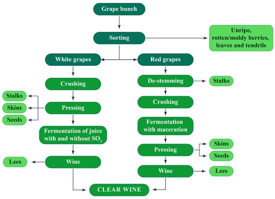
Figure 1.
Flowchart of the white and red winemaking processes.
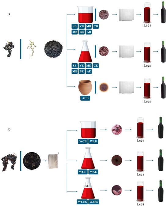
Figure 2.
Illustration of the different winemaking processes performed in beakers and Erlenmeyer flasks: (a) skin-contact macerated red wines; (b) no skin-contact fermented white wines with and without the addition of sulfur dioxide. For sample descriptions, see Table 1.
2.3. Physicochemical Standard Analysis
When the degree Brix (°Bx) of fermented juices was constant over 3 daily measurements, the pomace was hand-pressed through white sterilized double-layer gauze filters. The obtained wines were kept at 4 °C for 48 h and separated from the gross lees. Decanted wines were kept in filled green glass bottles with a capacity of 0.375 or 0.75 L and sealed with plastic-topped cork stoppers (T-corks) at 4 °C for two weeks before further chemical analysis. The standard oenological parameters of alcohol content (%, v/v), pH, total acidity (TA, expressed as g/L tartaric acid), and volatile acidity (VA, expressed as g/L acetic acid) were performed according to the Official Methods established by the European Community []. The concentration of ethanol by volume %(v/v) in the wine samples of 2020 and 2021 was determined by ebulliometry (Anadil, Anadia, Portugal). The pH values were obtained using a digital calibrated pH-meter (Thermo ScientificTM, Orion StarTM A211, Beverly, MA, USA). The determination of both total and free sulfur dioxide in wines was made by using the Sulfilyser semi-automatic apparatus (Laboratoires Dujardin-Salleron, Noizay, France) with the appropriate reagents and accessories, following the Ripper method []. Organic acids (malic and lactic acids) were determined by equipment OenoFoss™ (FOSS Iberia, Barcelona, Spain) using Fourier transform infrared spectroscopy (FTIR). Residual sugar (glucose and fructose) contents were measured with the Y25 enzymatic autoanalyser (Biosystems, Barcelona, Spain) []. All determinations were performed in duplicate.
2.4. Color and Phenolic Indexes
The chromatic characteristics of the wine samples were assessed following the spectrophotometric OIV-MA-AS2-07B method [], where the intensity of color is given by the sum of optical densities 420, 520, and 620 nm using a 10 mm optical path and the shade (N) is the ratio between absorbencies 420 and 520 nm. The values of the CIELAB color space (or simply CIE L*a*b* space) parameters were obtained according to the official method established by the International Organization of Vine and Wine []. The total polyphenol index (TPI) was determined by measuring the absorbance at 280 nm after dilution in water (1:100), according to Ribéreau-Gayon et al. []. The determination of anthocyanins was performed according to Ribéreau-Gayon et al. [] and Somers and Evans []. The degree of ionization of anthocyanins (α) (%), ionized anthocyanins (mg L−1 malvidin-3-O-glucoside), total pigments, polymerization index (%), and polymerized pigments were also determined, as described by Somers and Evans []. All spectrophotometric readings were carried out using the Cary 100 UV-Vis Spectrophotometer from Agilent Technologies (Mulgrave, Victoria, Australia).
2.5. Analysis of Aroma Composition by GC-FID
The determination of volatile compounds was analyzed in the laboratory using gas chromatography coupled with a flame ionization detector (GC-FID) method (6850 Series GC system, Agilent Technologies, Santa Clara, CA, USA), as described by Vaquero et al. []. Briefly, samples were injected after filtration through 0.45 µm cellulose methyl ester membrane filters (Phenomenex, Madrid, Spain). The column used was a DB-624 column. The total run time for each sample was 40 min. The carrier gas used was hydrogen and the internal standard (4-methyl-2-pentanol, 500 mg/L) (Fluka Chemie GmbH, Buchs, Switzerland). The detection limit was 0.1 mg/L. The volatile compounds analyzed with this technique were pre-calibrated with five-point calibration curves (r2). The concentration of volatile compounds in the samples is expressed as milligrams per liter (mg/L).
2.6. Microbiological Analysis of Ferments
After the end of fermentation, lees samples were kept in the refrigerator at 4 °C until further analysis. Five milliliters of the lees suspension was first mixed with 45 mL of Ringer Solution (Biokar Diagnostics, Pantin, France) and then serially diluted at a 9:1 dilution ratio. Each dilution was spread directly onto the surface of a GYP agar medium (20.0 g/L glucose (Merck, Darmstadt, Germany), 5.0 g/L yeast extract (Difco Laboratories, Detroit, MI, USA), 10.0 g/L peptone (Difco) and 20.0 g/L agar, pH 6.0). To avoid the growth of bacteria, chloramphenicol (Sigma, St. Louis, MO, USA) was added to the media at 100 mg L−1. The plates were incubated at 25.0 °C for seven days. After incubation, yeast colonies were purified and transferred to cycloheximide (100 mg L−1)-containing GYP agar plates. Yeast isolates showing growth on cycloheximide media are considered as non-Saccharomyces yeasts.
Identification at the genus and species levels was performed for the isolates following the protocol described by rDNA polymorphism of the 5.8s-ITS region []. Genomic DNA was isolated from cultures freshly grown on GYP agar medium according to standard procedures described by Chandra et al. []. Identification of the isolates was confirmed by sequencing the D1/D2 variable domains of the large subunit rRNA gene []. They were amplified using the external primers NL-1 (5′-GCATATCAATAAGCGGAGGAAAAG-3′) and NL-4 (5′-GGTCCGTGTTTCAAGACGG-3′). Polymerase Chain Reaction (PCR) products were purified and then sequenced directly (StabVida, Caparica, Portugal). A BLAST analysis “https://blast.ncbi.nlm.nih.gov/Blast.cgi (accessed on 30 June 2023)” was performed for the sequences obtained. Identification was considered valid when the identity was at least 98% []. The reported sequences have been deposited in the GenBank database, and their accession numbers are listed in Supplementary Table S1.
2.7. Statistical Analysis and Primary Data
2.7.1. Nonparametric Statistics
All statistical analyses were performed using R statistical software (v4.1.2) []. The data was originally recorded in Microsoft ® Excel Worksheets for Microsoft 365 MSO (Version 2406 Build 16.0.17726.20078) 64-bit and then imported into R. Prior to the ANOVA test (analysis of variance), the normality of data and the assumption of homogeneity of variances were tested statistically using the Shapiro–Wilk and Levene tests at 5% probability. When Levene’s test was significant (p < 0.05), nonparametric test procedures such as Kruskal–Wallis [,] and Conover-Iman tests [] came up as alternative solutions to deal with heterogeneous variances. The R package “PMCMRplus” [] was used to conduct the Conover-Iman post-hoc test and the “multcompView” package [] was used to carry out the mean differences of all pairwise multiple comparisons with letter-based representations in alphabetical order, respectively. The nonparametric Kruskal–Wallis test and the subsequent Conover-Iman test for contingency tables were conducted at a 95% confidence interval with a significance level of 5% (p < 0.05).
A nonparametric Spearman’s rank-order correlation coefficient test (rs) [] for the 2020 and 2021 wine parameters (physicochemical and CIELAB data, chromatic characteristics, and volatile compounds) was conducted to examine the possible relationships between the parameter mean values. Spearman’s correlation coefficient (rs) was defined from + 1 (perfect positive correlation) to −1 (perfect negative correlation), as described by Harutyunyan et al. []. The levels of statistical significance were as follows: 5% (p < 0.05), 1% (p < 0.01), 0.1% (p < 0.001), and 0.01% (p < 0.0001).
2.7.2. Principal Component Analysis (PCA) and Agglomerative Hierarchical Clustering (AHC)
Principal Component Analysis, or PCA, as a multivariate data statistical technique, was applied to assess the relationships between the average physical–chemical composition chromatic and phenolic characteristics of wines from two vintages (2020 and 2021). PCA was also carried out based on the 16 volatile compounds detected in the 2020 and 2021 wine samples. The base R function “prcomp” from the stats package [] was used to compute PCA on the scaling data (known as standardizing data). The bi-plot was plotted with the package ggbiplot [], and the R package ggplot2 [] was employed for data visualizations. An eigenvalue greater than one (the Kaiser-Guttman criterion) was considered for estimating the number of relevant principal components []. The factor loadings, either positive or negative, were categorized according to the magnitude of their absolute values: ‘strong’—the absolute value of the coefficient is greater than half of the maximum absolute value of the coefficient associated with the component; ‘moderate’—the absolute value of the coefficient lies between a quarter and a half of the largest absolute value, and finally ‘weak’—the absolute value is below a quarter of the largest absolute value. Negatively correlated contributions are displayed in parentheses []. The above categorization of PCA loadings is shown in the Supplemental Data File (Supplementary Tables S2–S7).
As a next step, agglomerative hierarchical clustering (AHC) analysis (Ward method of linkage and the Euclidean distances) [] was performed to cluster the 2020 and 2021 wine samples based on the similarity (closeness in terms of distance) of their chemical constituents. Before proceeding to clustering, it is essential to scale the data for better performance. The hierarchical tree, also known as a dendrogram, was analyzed and visualized using the “dendextend” R package [].
3. Results and Discussion
3.1. Grape Juice Yield and Chemical Composition
The berry weight, juice yields, and chemical composition of each grape variety for 2020 and 2021 are shown in Table 2. The juice yield obtained by hand pressing of V. sylvestris varied between 43 and 48% (v/w), lower than the yields of cultivated varieties and higher than the 15.4–16.3% and 16–17%, as reported by Loureiro et al. [] and Maghradze et al. [], respectively. This resulted from the higher proportion of skins due to the smaller berry size of V. sylvestris. Compared to the wild variety, it is interesting to note that Vinhão as a teinturier grape (i.e., accumulates anthocyanins both in the berry skin and in the pulp) attained higher anthocyanin concentration, while Marufo, Melhorio, and Castelão showed the lowest contents. Melhorio showed remarkably high total acidity (g/L tartaric acid) comparable to that of V. sylvestris. The other non-teinturier cultivated varieties showed intermediate values for all the parameters assessed.
Table 2.
Chemical composition of juices of wild grapevines and several red grape cultivars (Vitis vinifera L.) during 2020 and 2021.
In comparable reports, Maghradze et al. [] described a similar concentration of sugar (25.1 °Bx/15.7% probable alcohol) and pH 3.4 in Georgian wild grapes with a lower total acidity (7.8 g/L). Another autochthonous Georgian cultivar ‘Saperavi’ with dark skins and flesh (teinturier variety), yielded 22.1 °Bx and pH 3.2 but a high total acidity (tartaric acid) of 9.2 g/L []. On the other hand, Loureiro et al. [] reported a very low sugar content in Spanish wild grapevine populations (12.7 to 13.9 °Bx).
3.2. Yeast Isolation and Identification
A total of 82 isolates were subjected to molecular identification, showing that all strains belonged to S. cerevisiae, except for one strain of Zygosaccharomyces bailii in Castelão red wine (Supplementary Table S1). The presence of S. cerevisiae was expected since it is the main agent of wine alcoholic fermentation, irrespective of the vessel shape. The presence of Z. bailii is also common at the end of fermentation and may originate from grapes or soil [].
3.3. Physicochemical Analysis
The spontaneous fermentation led to the obtention of wines with different volatile acidities and ethanol. Most of the fermentation performed in beakers yielded higher volatile acidity and low ethanol, consistent with a lower fermentation performance (Table 3). This may be explained by the different microbial activities present in spontaneous grape juice fermentation []. The variability in these fermenting volatile patterns might have been reduced by the addition of sulfite and the use of S. cerevisiae as starter cultures. Indeed, Harutyunyan et al. [] performed controlled inoculated fermentations in open vessels, and the final wines had low volatile acidity levels (0.21 to 0.50 g/L expressed in acetic acid). However, this would not mimic the conditions of the earliest fermentations, where acetic acid bacteria may have begun to produce acetic acid in a process similar to sour rot in grapes []. In addition, non-Saccharomyces strains present at the onset of fermentation diverted carbon away from ethanol production []. In combination, S. cerevisiae may also have produced higher volatile acidity due to increased oxygen exposure []. Thus, acetic acid spoilage was more likely to occur in these types of vessels with wide surface contact with air. Interestingly, fruit flies, which are known vectors of acetic bacteria [], were numerous over beaker ferments but were seldom observed inside the Erlenmeyer flasks, indicating that the CO2 released did not efficiently protect the juices. The remaining chemical parameters did not show any dependence on the shape of the vessel (Tables S8 and S9 of the Supplementary Materials).
Table 3.
Volatile acidity and ethanol content at the end of juice spontaneous fermentation in beakers and Erlenmeyer flasks during the harvests of 2020 and 2021.
A recent study by Loureiro et al. [] reported a low alcoholic degree in Spanish wild grapevine wines, varying between 6.2% and 7.1% (v/v). Another study carried out by Maghradze et al. [] showed low concentrations of ethanol in wild grapevine wines from the Southern Caucasus region, ranging from 3.63% to 10.15%. Analysis of volatile acidity was not carried out, and it might have provided an explanation for the high total acidity when tartaric acid and malic acid were low, even though lactic acid production may occur []. This author and colleagues showed higher ethanol content (14.2%) and low volatile acidity (0.5 g/L) in wines produced from wild grapes []. Ocete et al. [] also reported a low concentration of ethanol, not exceeding 11%. In addition, Drori et al. [] reported moderate to high ethanol concentrations ranging from 11.2% to 14.4%. The current study also revealed low to moderate contents of ethanol (8.50% and 12.35%) in V. sylvestris wines (Tables S8 and S9). Regarding domesticated wines, Goulioti et al. [] showed that the alcohol strength in Greek Xinomavro wines ranged from 12.9 to 13.9% (v/v), consistent with those of Vinhão and Marufo with small variations (Table S8).
The mean values from the standard physical–chemical, and CIELAB parameters of the 2020 and 2021 wines, followed by the results of multiple comparisons (via Kruskal–Wallis test) between the groups and pairwise comparisons (via Conover-Iman test) for all possible pairwise multiple comparisons between samples are presented in Supplementary Tables S8 and S9. Statistically significant differences were detected between the groups by the Kruskal–Wallis test (p < 0.05). In addition, the Conover-Iman post-hoc test showed significant pairwise differences (p < 0.05) (Tables S8 and S9).
After performing nonparametric tests for group and pairwise comparisons, Spearman’s rho correlation coefficients were simultaneously calculated between all parameters. The correlation matrix is shown in Table 4. Although the correlation does not imply causation, predictable high correlations were found among the values of volatile acidity (VA), total acidity (TA), and pH in 2021. For instance, total acidity was highly and positively correlated with volatile acidity (r = +0.79, p < 0.01) and negatively correlated with pH (r = −0.75, p < 0.01), both induced by acetic acid overproduction. With ethanol, TA showed a very high relationship, where the coefficient was negative (r = −0.89) at the 0.01 level. Next, a strong negative correlation was also observed between ethanol and volatile acidity (r = −0.75, p < 0.01) in 2021, reflecting lower ethanol production because of the aforementioned shift in carbon metabolism. The above-mentioned parameters did not show any relationship with each other in 2020, reflecting the performance unpredictability of spontaneous fermentation. Inoculated fermentation showed naturally high production of sulfur dioxide up to 60 mg/L, as observed by Harutyunyan et al. [] in white juices. In 2020, total sulfite showed a high inverse association with volatile acidity (r = −0.78, p < 0.01), indicating that the sulfur dioxide produced during fermentation might have an action against acetic acid bacteria or non-Saccharomyces yeasts in combination with grape phenolics []. Aside to be added, Cuijvers et al. [] reported that in spontaneous wine fermentation, the concentration of SO2 below 40 mg/L and concentrations between 60 and 100 mg/L inhibit the growth of unwanted non-Saccharomyces yeast species. Accordingly, white-style fermentation of Tempranillo Tinto juice yielded higher volatile acidity. In the case of 2021, besides total, also free sulfite was moderately and inversely associated with volatile acidity (ranging from 0.65 to 0.58) at p < 0.05 level. In 2020 and 2021, there were high and very high positive associations of total and free sulfite with chroma (C*) (p < 0.01 and p < 0.0001), which is in accordance with the sulfite antioxidant properties [,]. The latter was moderately and negatively correlated with volatile acidity and hue (H*), yielding coefficients that fell below 0.70 (Table 4). As for organic acid and sugar contents, samples showed unfinished fermentation when sugar was higher than 2 g/L (Supplementary Table S10), probably due to the combined inhibitory effect of initial high sugar and acetic acid production []. In 2020, malolactic fermentation was practically absent, whereas in 2021, the conversion of malic acid into lactic acid had already begun at the end of the experiments (Table S10), confirming the above-mentioned performance unpredictability of spontaneous fermentations.
Table 4.
Pairwise Spearman’s rank-order correlation matrix of standard physical–chemical, and CIELAB parameters of all wines.
For better visualization of the data from both years (2020–2021), principal component analysis (PCA) was performed to identify the relationships among the mean values of the eight measured variables (Figure 3 and Figure 4). As displayed in Figure 3, the first two PCs explained 76.5% of the total variance of the entire dataset. This is an acceptably large percentage of variation. With the addition of the third component (PC3) system, it increased up to 89.8%. The first principal component (PC1) yielded the highest variation (49.4%) and had a strong positive loading for pH and strong negative loadings for free SO2, total SO2, and chroma (C*). The second principal component (PC2) yielded the lowest variation (27.1%) and had strong negative loadings for volatile acidity and total acidity. Finally, the third principal component (PC3) made a small contribution (13.3%) to the total variation in the data and was dominated by a large negative loading for hue (H*) (Table S2). The correlation between the variables was also described. Ethanol and pH were positively correlated to each other. A positive correlation was also found between parameters such as C*, total SO2, and free SO2. Volatile acidity and free SO2 were negatively correlated to each other.
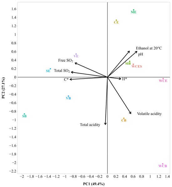
Figure 3.
Bi-plot of the Principal Component Analysis (PCA) with the main physicochemical parameters of the 2020 wines (sample description in Table 1). The small and large angles between the corresponding variables represent the degree of relationships. The vector lengths indicate the strength of the correlation (closeness) of the corresponding parameter with the experimental samples. The percentage values (in parentheses) represent the proportion of explained variance for each principal component.
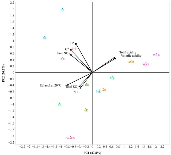
Figure 4.
Bi-plot of the Principal Component Analysis (PCA) with the main physicochemical parameters of the 2021 wines (sample description in Table 1). The small and large angles between corresponding variables represent the degree of relationships. The vector lengths indicate the strength of the correlation (the closeness) of the corresponding parameter with the experimental samples. The percentage values (in parentheses) represent the proportion of explained variance for each principal component.
The chemical similarity of different samples was further illustrated by cluster analysis (AHC), and the resulting tree-like dendrogram is shown in Supplementary Figure S1 (cf., Table S8). Three clusters of their measured attributes have been obtained. The first cluster combined SB, SE, VB, and VE, the second cluster CB and WCB, and the third WCE, MB, WCES, ME, and CE, respectively. It can be seen that VB and VE, as well as MB and WCES, are the most similar objects, as they are joined by the shortest height link.
As shown in Figure 4, the first two principal components explained 68.3% of the total variability in the entire dataset. With the addition of the third component (PC3), it increased up to 83.3%. The first axis (PC1) yielded the highest variation (47.8%) and had strong positive loadings for volatile acidity and total acidity and strong negative loadings for ethanol, free SO2, and chroma (C*). The second axis (PC2) yielded the lowest variation (20.5%) and had strong positive loadings for chroma (C*), hue (H*), and free SO2. Finally, the third axis (PC3) made a small contribution (15.0%) to the total variation of the data and was dominated by a large positive loading for total SO2 and a large negative loading for pH (Table S3). The PCA bi-plot showed that total acidity and volatile acidity were positively correlated with each other and negatively correlated with ethanol. Similarly, a positive correlation was also observed between total SO2 and pH. The correlations among other parameters, such as free SO2, chroma, and hue were found to be positive.
The results of the cluster analysis in the form of a dendrogram are presented in Supplementary Figure S2 (cf., Table S9). Similarity-based four clusters were obtained. The first cluster combined WAB, ACB, and WAE, the second cluster combined WAES, the third cluster combined SB and SE, and the fourth cluster combined MB, ME, AB, AE, VB, VE, BB, and BE. It can be seen that MB and ME, as well as VB and VE, are the most similar objects, as they are joined by the shortest height link.
Overall, the cluster analysis of both vintages showed an unexpected correspondence with the grape variety, given the heterogeneity of spontaneous fermentation.
3.4. Spectrophotometric Determinations
The average values from the color and phenolic indexes of the 2020 and 2021 wines, followed by multiple comparisons (by Kruskal–Wallis test) between the treatment groups, and pairwise comparisons (by Conover-Iman test) for all possible pairwise multiple comparisons between samples are presented in Supplementary Tables S11 and S12. In the Kruskal–Wallis test, significant differences between all groups in the observed variables were found at the 5% significance level. Additionally, the Conover-Iman post-hoc test for pairwise comparisons revealed significant differences (p < 0.05) (Tables S11 and S12).
As shown in Tables S11 and S12, the V. sylvestris wines are characterized by high values of color intensity varying between 27.33 AU and 64.46 AU. Similarly, previously published research has also shown high color intensity in wines made from wild grapes [,,,].
For comparison with V. vinifera wines, Vinhão (teinturier grapes) presented remarkably high color intensity values ranging from 70.22 AU to 144.56 AU. Giacosa et al. [] reported average wine color intensities obtained from Italian cultivated varieties in the range from 4.02 AU (‘Corvina’) to 14.82 AU (‘Teroldego’). The present study also revealed the same range of values for wines from Marufo, Castelão, Melhorio, and Tempranillo Tinto. In this most recent study, Goulioti et al. [] reported low values of color intensity in Greek Xinomavro wines between 2.3 AU and 5.9 AU, which are in agreement with the values of Marufo and Melhorio (Tables S11 and S12).
Next, the pairwise relationships between all variables were determined by Spearman’s correlation coefficient. The correlation matrix is presented in Table 5. Most of the correlation coefficients were statistically significant. Spearman correlation test revealed a very high positive correlation between color intensity and anthocyanins (r = +0.92), total anthocyanins (r = +0.95 and +0.91), ionized anthocyanins (r = +0.98 and +0.99), total pigments (r = +0.97 and +0.93), and polymerized pigments (r = +0.99 and +0.93) at the 0.01 significance level. On the contrary, relatively low correlations were found between the color intensity and the degree of ionization of anthocyanins and the polymerization index. Probably, because anthocyanins are not stable, breakdown reactions are possible under uncontrolled spontaneous fermentation, as observed by Pfahl et al. [] under the influence of oxygen during barrel aging.
Table 5.
Pairwise Spearman’s rank-order correlation matrix of the 2020 and 2021 wines’ chromatic characteristics.
Another color-defining parameter, the shade (N), showed very strong negative correlations with total anthocyanins (r = −0.95), ionized anthocyanins (r = −0.94), total pigments (r = −0.95), and polymerized pigments (r = −0.91) at the 0.1 and 0.01 significance levels. This parameter also showed a very strong correlation with color intensity (r = −0.92, p < 0.0001). The latter was moderately and positively correlated with the degree of ionization of anthocyanins, yielding a coefficient below 0.70 (p < 0.05).
In 2021, the highest degree of positive correlation was observed between the total phenol index and polymerized pigments (r = +0.96, p < 0.0001). For all other parameters, the total phenol index showed statistically significant but moderate and strong positive relationships. Similar to the total phenol index, the highest degrees of positive relationships were also found between the values of anthocyanins, total anthocyanins, ionized anthocyanins, total pigments, and polymerized pigments at the 0.01 significance level.
Overall, the positive correlations of most spectrophotometric indexes in both vintages were expected [,].
Principal component analysis (PCA) was carried out to characterize the 2020 and 2021 wines in relation to their color and phenolic characteristics (Figure 5 and Figure 6). As can be seen from Figure 5, the PC1 and PC2 captured 73.5% and 14.2% of the variations in the dataset. The corresponding cumulative amount of explained variance by the first two principal components is 87.7%, determined by ten variables, and by three PCs is 99% if it is also added. The first axis (PC1) yielded the highest variation (73.5%) and had strong positive loadings for intensity, total phenol index, total anthocyanins, ionized anthocyanins, total pigments, and polymerized pigments. The second axis (PC2) yielded the lowest variation (14.2%) and had strong positive loadings for shade and polymerization index but large negative loadings for anthocyanins. Finally, the contribution of the third axis (PC3) to the total variation was small (11.3%) compared with those of PC1 and PC2 and was dominated by a large positive loading for the polymerization index (Table S4). Several positive associations were observed between intensity, total anthocyanins, ionized anthocyanins, total pigments, and polymerized pigments. A negative association was found between the polymerization index and anthocyanins.
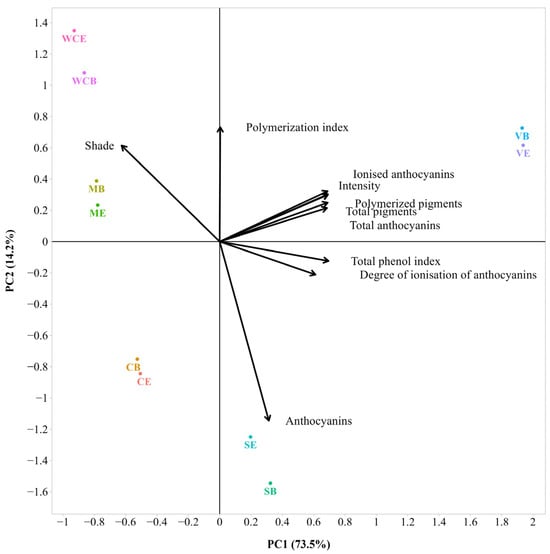
Figure 5.
Bi-plot of the Principal Component Analysis (PCA) of chromatic analysis for the 2020 wines without WCES (sample description in Table 1). The small and large angles between corresponding variables represent the degree of relationships. The vector lengths indicate the strength of the correlation (the closeness) of the corresponding parameter with the experimental samples. The percentage values (in parentheses) represent the proportion of explained variance for each principal component.
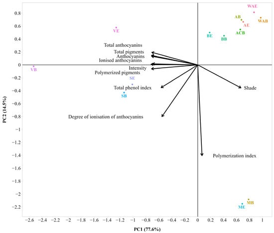
Figure 6.
Bi-plot of the Principal Component Analysis of chromatic analysis (PCA) for the 2021 wines without WAES (sample description in Table 1). The small and large angles between corresponding variables represent the degree of relationships. The vector lengths indicate the strength of the correlation (the closeness) of the corresponding parameter with the experimental samples. The percentage values (in parentheses) represent the proportion of explained variance for each principal component.
Agglomerative hierarchical clustering (AHC), without sulfite (WCES), revealed that the 2020 wines were grouped according to their varietal origin, regardless of the fermentation vessel (Supplementary Figure S3) (cf., Table S11). Three clusters were obtained. The first cluster combined VB and VE, the second cluster combined SB and SE, and the third cluster combined WCB, WCE, CB, CE, MB, and ME. The wine samples (VB and VE) in the first cluster were more similar to each other than those in the other clusters. The next two most similar samples are CB and CE, as they are joined by the shortest height link.
The PC1 and PC2 captured 77.6% and 14.5% of the variations in the dataset, shown in Figure 6. Approximately two-thirds of the data are represented by the first (main) component. The corresponding cumulative amount of explained variance by two PCs is 92.1%, which is enough to accurately represent the data. Color intensity, anthocyanins, total anthocyanins, ionized anthocyanins, total pigments, and polymerized pigments have strong negative loadings on component 1. All of these parameters showed positive correlations with each other. Shade had a strong positive loading on component 1 and was negatively correlated with total anthocyanins. The degree of ionization of anthocyanins and polymerization index had large negative loadings on component 2 (Table S5).
In 2021, the dendrogram tree produced from the AHC-based method for clustering was drawn without the sample (WAES) to which sulfite was added, given that it would not be a full spontaneous fermentation (Supplementary Figure S4) (cf., Table S12). Four clusters were obtained. The first cluster combines MB and ME; the second cluster combines BB, BE, WAB, WAE, ACB, AB, and AE; the third combines VB; and the fourth combines VE, SB, and SE. The wine samples (AB and AE) in the second cluster were more similar to each other than those in the other clusters, as they were joined by the smallest height link.
Overall, the results of both vintages showed the stability of phenolic spectrophotometric indexes even under different spontaneous fermentation heterogeneities. For instance, Tempranillo Tinto and Castelão wines were similarly clustered even when fermented with skins or without skins. Then, the results are in accordance with the suitability of using phenolic composition to discriminate wines from different grape varieties []. Sen and Tokatli [] and Basalekou et al. [] also showed that wines can be distinguished from grape varieties according to their phenolic composition and color characteristics. Recently, Maghradze et al. [] found that high color intensity (CI) and total polyphenol index (TPI) are characteristic of wines from wild grapevines growing in the South Caucasus.
3.5. Volatile Compounds Production
For 2020 volatiles, nonparametric tests (the Kruskal–Wallis test and the Conover-Iman post-hoc test) were not performed as samples were reported without repetitions (Supplementary Table S13). The average data of estimated volatile compounds (VOCs) of the 2021 wines, followed by multiple comparisons (Kruskal–Wallis test) between the treatment groups, and pairwise comparisons (Conover-Iman test) for all possible pairwise multiple comparisons between samples are presented in Supplementary Table S14. Statistically significant differences were found between treatments (p < 0.05, Kruskal–Wallis test), and the subsequent post-hoc analysis using the Conover-Iman test revealed significant pairwise differences (p < 0.05) (Table S14). Nevertheless, the volatile composition of the wines from both vintages was comparable to that reported in different wines by Stój et al. [], Martins et al. [], and Vaquero et al. [].
After group and pairwise comparisons, nonparametric Spearman’s rho correlation coefficients were used to assess the relationships between all paired variables. The correlation matrixes of wine-derived volatile compounds from the 2020 and 2021 vintages are shown in Table 6 and Table 7, illustrating the variability of volatile production in spontaneous fermentations. Indeed, most of the correlation coefficients were not statistically significant (Table 6 and Table 7).
Table 6.
Pairwise Spearman’s rank-order correlation matrix of volatile contents in the 2020 wine samples.
Table 7.
Pairwise Spearman’s rank-order correlation matrix of volatile contents in the 2021 wine samples.
In 2020, the Spearman correlation test revealed a strong positive relationship between methanol and secondary alcohols, such as 3-methyl-1-butanol (r = +0.86, p < 0.001) and 2,3-butanediol (r = +0.80, p < 0.01). With 2-methyl-1-butanol (r = +0.91, p < 0.001) and 2-phenylethanol (r = +0.92, p < 0.0001), methanol showed very strong positive relationships. In addition to these positive relationships, methanol also showed a strong negative correlation with ethyl acetate (r = −0.81, p < 0.01). In the case of the primary alcohol 2-phenylethanol, we observed a very strong and positive correlation with 2,3-butanediol (r = +0.91, p < 0.001). 2-phenyl ethanol was highly and positively correlated with pentanol isomers 2-methyl-1-butanol (r = +0.87, p < 0.001) and 3-methyl-1-butanol (r = +0.77, p < 0.01) and moderately negatively correlated with ethyl acetate (r = −0.66, p < 0.05), while the latter was found to be highly negatively correlated with 2-methyl-1-butanol (r = −0.73, p < 0.05).
Accordingly, in the 2021 correlation matrix (Table 7), only a few pairs of volatile compounds turned out to be statistically significant at different levels. For instance, the methanol content was moderately and positively associated with 1-propanol (r = +0.56), ethyl lactate content (r = +0.57), and 2,3-butanediol content (r = +0.58) at the 5% significance level (p < 0.05). A moderate negative association was found between methanol and acetaldehyde content (r = −0.63, p < 0.05). Another aroma compound, 3-methyl-1-butanol, was highly and positively correlated with isobutanol (r = +0.78, p < 0.01) and 2-methyl-1-butanol (r = +0.82, p < 0.001) and negatively correlated with ethyl acetate (r = −0.78, p < 0.001). There was a moderate positive correlation between isobutanol and 2-methyl-1-butanol content (r = +0.67, p < 0.01). Interestingly, we did not observe any relationship at the 0.01% significance level.
The most significant coincidence in both vintages was the inverse correlation between ethyl acetate and 2- or 3-methyl-1-butanol. Probably, this may correspond to the yeasts producing 3-methyl-1-butanol, while bacteria were closely related to the formation of ethyl acetate, as observed by Han and Du [] in apple cider fermentation.
Further, a multivariate principal component analysis (PCA) was carried out to characterize the 2020 and 2021 wines in relation to their volatile aroma composition (Figure 7 and Figure 8). As can be seen in Figure 7, PC1 accounted for 38.2%, and PC2 accounted for 20.1% of the total variations within the dataset. The cumulative amount of variance explained by two PCs was 58.3%, followed by three PCs (72.3), four PCs (82.3), and five PCs (88.9). The first axis (PC1) has strong positive loadings for methanol, 1-propanol, 2-methyl-1-butanol, and ethyl lactate. The second axis (PC2) has strong negative loadings for isoamyl acetate, isobutyl acetate, and 2-phenylethyl acetate. The third axis (PC3), with a small contribution of 14.0%, is dominated by a large positive loading for hexanol. The remaining components (PC4 and PC5), with minor contributions to the total variation, arranged in descending order, are presented in Supplementary Table S6. The bi-plot shows that isobutyl acetate and 2-phenyl ethyl acetate were positively correlated with each other. A positive correlation was also observed between 1-propanol and ethyl lactate. There was a negative correlation between isobutanol and isoamyl acetate. A negative correlation was also found between 3-methyl-1-butanol and ethyl acetate. A Principal component analysis (PCA) by Martins et al. [] showed a clear separation among the different types of wine (e.g., red, white, and palhete) based on their volatile composition (31% of the variance by the two principal components), particularly among red and white ones.
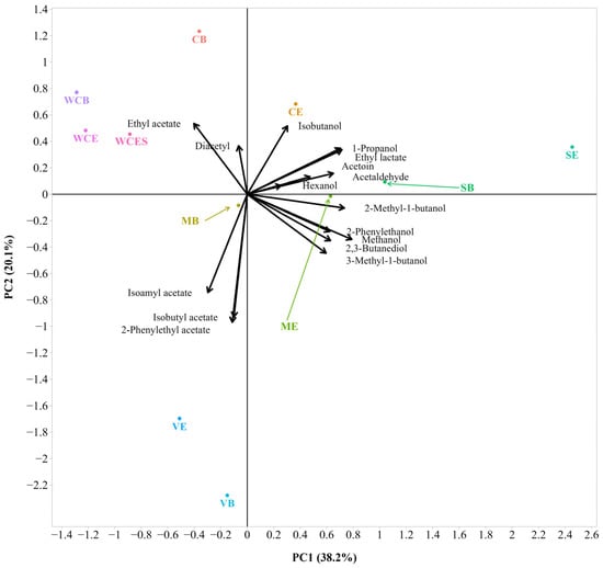
Figure 7.
Bi-plot of the Principal Component Analysis (PCA) with volatile aroma composition of the 2020 wines (sample description in Table 1). The small and large angles between corresponding variables represent the degree of relationships. The vector lengths indicate the strength of the correlation (the closeness) of the corresponding parameter with the experimental samples. The percentage values (in parentheses) represent the proportion of explained variance for each principal component. The colored lines are used to connect some data labels to their respective points in order to avoid overlapping (SB, MB, and ME).
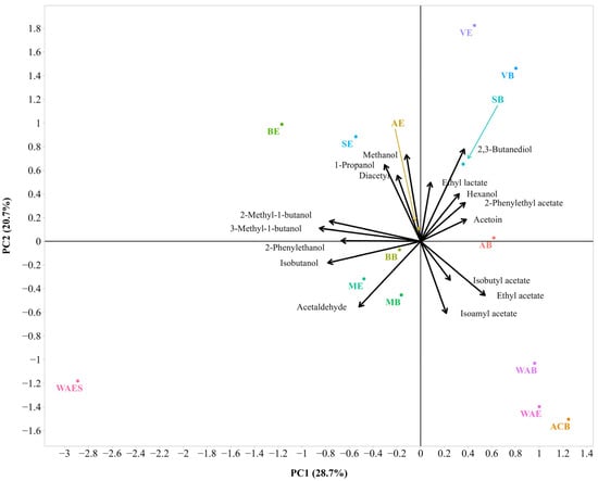
Figure 8.
Bi-plot of the Principal Component Analysis (PCA) with volatile aroma composition of the 2021 wines (sample description in Table 1). The small and large angles between corresponding variables represent the degree of relationships. The vector lengths indicate the strength of the correlation (the closeness) of the corresponding parameter with the experimental samples. The percentage values (in parentheses) represent the proportion of explained variance for each principal component. The colored lines are used to connect some data labels to their respective points in order to avoid overlapping (SB and AE).
The results of cluster analysis of the compositions of the 16 volatile compounds determined for the 2020 and 2021 wines are shown in Supplementary Figures S5 and S6 (cf. Tables S13 and S14). As shown in Figure S5 (cf., Table S13), five clusters were obtained: (i) SB and SE, (ii) VB and VE, (iii) CE, MB, and ME, (iv) CB, and (v) WCB, WCE, and WCES. The samples WCE and WCES that are grouped into the fifth cluster are very similar to each other since they are aggregated at a small height.
As shown in Figure 8, PC1 accounted for 28.7%, and PC2 accounted for 20.7% of the variations within the dataset. The cumulative variance explained by two PCs was 49.4%, followed by three PCs (63.5), four PCs (75.1), and five PCs (84.1). Isobutanol, 2-methyl-1-butanol, 3-methyl-1-butanol, and 2-phenylethanol had strong negative loadings on component 1. Methanol, 1-propanol, and 2,3-butanediol had strong positive loadings on component 2, while isoamyl acetate had a strong negative loading on component 2. Ethyl acetate, acetoin, isoamyl acetate, and 2-phenylethyl acetate had strong positive loadings on component 3 (Table S7). Correlation analysis showed that 2-methyl-1-butanol and 3-methyl-1-butanol were positively correlated. Positive associations were also observed among methanol, 1-propanol, and diacetyl content. The latter were inversely correlated with isoamyl acetate. Acetaldehyde also showed an inverse association with hexanol and 2-phenylethyl acetate.
Four clusters were obtained: (i) WAES, (ii) ACB and WAE, (iii) WAB, SB, BB, MB, ME, AB, and AE, and (iv) SE, BE, VB, and VE (Supplementary Figure S6) (cf., Table S14). In Figure S6, the MB and ME samples in the third cluster are similar to each other.
Overall, the cluster results of both vintages are in accordance with Stój et al. [], who reported grape variety as the factor with a higher impact on the volatile composition in yeast-inoculated fermentations. This similarity should have reflected the composition of different volatile precursors according to variety. These precursor-dependent volatiles were not as strongly influenced by vessel shape as acetic acid production was dependent on microbial activity. Probably, the dominance of S. cerevisiae at the end of fermentations (see Table S1 of the Supplementary Materials) explains the similarity of results from inoculated and non-inoculated fermentation.
4. Limitations and Future Research
Non-porous surface glass containers were used to conduct experiments despite the absence of this material in the AShSh and BB cultures. The reason was to reduce the likely influence of the nature of the clay porosity, which might overwhelm the influence of the vessel’s shape. Indeed, one experiment was carried out in a ceramic container with a more porous surface, yielding even higher volatile acidity. The second limitation concerns the lack of analysis of acetic acid bacteria (AAB) and non-Saccharomyces yeasts, which could explain the different fermentation performances. It would also be interesting to perform sensory analysis techniques (mainly for porous clay containers as they affect the sensory profiles of wines), but the small quantity of V. sylvestris grapes did not provide enough wine. Nevertheless, the chemical composition of these wines justifies further studies. Moreover, the high acidity shared by Melhorio should be explored under the topic of adaptation to climate change conditions. The suitability of other almost extinct varieties like Branjo to increase the diversity of wines paves the way for further studies of other indigenous minority varieties.
Further studies should also evaluate (i) the impact of different coatings (e.g., epoxy resin, pine resin or pitch, beeswax) of clay-based ceramics on the chemical composition of wine, mainly the volatile composition, (ii) the effect of in-amphorae aging on wine’s sensory profile compared to different types of aging tank containers such as stainless steel, new and used oak barrels, barriques and glass bottles, and (iii) the oxygen transmission rate (OTR) in different materials suitable for wine fermentation and maturation.
5. Conclusions
The comparative study of vessel shapes is particularly interesting from an archaeological point of view. The overall results showed that the shape of the vessels did influence the performance of fermentation. There was a tendency for lower volatile acidity in conical Erlenmeyer flasks, corroborating the hypothesis that the shape of the vessels favored wine acetification or, at least, contributed to a higher incidence of vinegary wines in open-mouth vessels. Therefore, against the backdrop of experimental archaeology, the results showed that the shape of the vessels may explain why the earliest beverages similar to present wines were more likely to appear in the South Caucasus (the cradle of ancient winemaking) rather than in the Iberian Peninsula, even if in both regions grapes from V. sylvestris were available to indigenous populations. In this way, wines in transport amphorae brought by Phoenician settlers or traders (Phoenician elites) would have been more appreciated by Iberian elites than by local beverages, opening the way for a broad range of prosperous economic activities as a result of colonial interaction from this period onwards.
This work also presents results that impact the future development of the wine industry related to (i) the present interest in indigenous grape varieties to cope with climate change and (ii) the commercial appeal of the rebirth of minority grapevine varieties.
Supplementary Materials
The following supporting information can be downloaded at https://www.mdpi.com/article/10.3390/fermentation10080401/s1, Table S1: Yeast isolates from the 2020 wine lees after spontaneous fermentation. Table S2: Simplified version of the principal component (PC) coefficients for the main physical–chemical, and CIELAB parameters of the 2020 wines. Table S3: Simplified version of the principal component (PC) coefficients for the main physical–chemical, and CIELAB parameters of the 2021 wines. Table S4: Simplified versions of the principal component (PC) coefficients for the chromatic characteristics of the 2020 wines. Table S5: Simplified version of the principal component (PC) coefficients for the chromatic characteristics of the 2021 wines. Table S6: Simplified version of the principal component (PC) coefficients for the volatile contents of the 2020 wines. Table S7: Simplified version of the principal component (PC) coefficients for the volatile contents of the 2021 wines. Table S8: Means and standard deviations (SDs) of standard physical–chemical and CIELAB parameters of the 2020 wines, followed by the results of the Kruskal–Wallis (Chi-square, df, p-value) and the Conover-Iman tests. Table S9: Means and standard deviations (SDs) of standard physical–chemical and CIELAB parameters of the 2021 wines, followed by the results of the Kruskal–Wallis (Chi-square, df, p-value) and the Conover-Iman tests. Table S10: Analysis at the end of fermentation for the wines from the harvests of 2020 and 2021. Table S11: Means and standard deviations (SDs) of the 2020 wines’ chromatic characteristics, followed by the results of the Kruskal–Wallis (Chi-square, df, p-value) and the Conover-Iman tests. Table S12: Means and standard deviations (SDs) of the 2021 wines’ chromatic characteristics, followed by the results of the Kruskal–Wallis (Chi-square, df, p-value) and the Conover-Iman tests. Table S13: Volatile composition of the 2020 wine samples. Table S14: Means and standard deviations (SDs) of the composition of volatile compounds in the analyzed wine samples in 2021, followed by the results of the Kruskal–Wallis (Chi-square, df, p-value) test and the Conover-Iman test. Figure S1: Dendrogram of the hierarchical clustering analysis (HCA) of the 2020 wine physical–chemical and CIELAB parameters (sample description in Table 1). The red-dashed rectangles around the branches show the corresponding clusters marked by different colors. The height at which two branches are linked together reflects the distance between the wines/clusters; the smaller the height, the more similar the wines/clusters are. Figure S2: Dendrogram of the hierarchical clustering analysis (HCA) of physical–chemical analysis and CIELAB parameters of the 2021 wine samples (see Table 1 for sample description). The red-dashed rectangles around the branches show the corresponding clusters, marked by different colors. The height at which two branches are linked together reflects the distance between the wines/clusters; the smaller the height, the more similar the wines/clusters are. Figure S3: Dendrogram of hierarchical clustering analysis (HCA) of chromatic analysis of the 2020 wine samples (sample description in Table 1). The red-dashed rectangles around the branches show the corresponding clusters, marked by different colors. The height at which two branches are linked together reflects the distance between the wines/clusters; the smaller the height, the more similar the wines/clusters are. Figure S4: Dendrogram of hierarchical clustering analysis (HCA) of the 2021 wine chromatic characteristics (see Table 1 for sample description). The red-dashed rectangles around the branches show the corresponding clusters, marked by different colors. The height at which two branches are linked together reflects the distance between the wines/clusters; the smaller the height, the more similar the wines/clusters are. Figure S5: Dendrogram of hierarchical clustering analysis (HCA) of the volatile composition of the 2020 wine samples (sample description in Table 1). The red-dashed rectangles around the branches show the corresponding clusters, marked by different colors. The height at which two branches are linked together reflects the distance between the wines/clusters, the smaller the height the more similar the wines/clusters are. Figure S6: Dendrogram of hierarchical clustering analysis (HCA) of the volatile analysis of 2021 wine samples (see Table 1 for sample description). The red-dashed rectangles around the branches show the corresponding clusters, marked by different colors. The height at which two branches are linked together reflects the distance between the wines/clusters, the smaller the height the more similar the wines/clusters are.
Author Contributions
Conceptualization, M.M.-F. and M.H.; methodology, All; software, M.H. and A.A.; validation, M.M.-F. and M.H.; formal analysis, M.H.; investigation, All; resources, M.M.-F.; data curation, M.M.-F.; writing—original draft preparation, M.H.; writing—review and editing, M.M.-F. and M.H.; visualization, M.M.-F.; supervision, M.M.-F.; project administration, M.M.-F.; funding acquisition, M.M.-F. All authors have read and agreed to the published version of the manuscript.
Funding
This work was conducted under financial support by the “Armenian Communities Department” of the Fundação Calouste Gulbenkian (Lisbon, Portugal) within the scope of the Short-Term Grant for Armenian Studies, grant number 214070/2023 (https://gulbenkian.pt/en/bolsas-lista/short-term-grant-for-armenian-studies/, accessed on 4 June 2024); and by national funds through FCT (Fundação para a Ciência e a Tecnologia, I.P.; Lisbon, Portugal), in the scope of the project Linking Landscape, Environment, Agriculture and Food Research Centre (Ref. UIDB/04129/2020 and UIDP/04129/2020).
Institutional Review Board Statement
Not applicable.
Informed Consent Statement
Not applicable.
Data Availability Statement
All data used in this study are included in the manuscript and/or its supporting information files.
Acknowledgments
The authors are grateful to Pedro Silva from the University of Lisbon’s School of Agriculture (ISA) for statistical consultation. Researcher-archaeologist Boris Gasparyan from the Institute of Archaeology and Ethnography, NAS RA, is deeply acknowledged for daily consultations, constructive comments, and suggestions. Many thanks to Dois Portos Oenological Station (INIAV), Vinilourenço (Douro region), and Casa Santos Lima (Lisbon region) companies for supplying the grapes. This study is dedicated to the renowned Armenian viticulturist Gagik Melyan, who unfortunately passed away.
Conflicts of Interest
The authors declare no conflicts of interest.
References
- Harutyunyan, M.; Malfeito-Ferreira, M. The rise of wine among ancient civilizations across the Mediterranean basin. Heritage 2022, 5, 788–812. [Google Scholar] [CrossRef]
- Dong, Y.; Duan, S.; Xia, Q.; Liang, Z.; Dong, X.; Margaryan, K.; Musayev, M.; Goryslavets, S.; Zdunić, G.; Bert, P.-F.; et al. Dual domestications and origin of traits in grapevine evolution. Science 2023, 379, 892–901. [Google Scholar] [CrossRef] [PubMed]
- McGovern, P.; Jalabadze, M.; Batiuk, S.; Callahan, M.P.; Smith, K.E.; Hall, G.R.; Kvavadze, E.; Maghradze, D.; Rusishvili, N.; Bouby, L.; et al. Early Neolithic wine of Georgia in the South Caucasus. Proc. Natl. Acad. Sci. USA 2017, 114, E10309–E10318. [Google Scholar] [CrossRef] [PubMed]
- Sagona, A. The Archaeology of the Caucasus: From Earliest Settlements to the Iron Age; Cambridge World Archaeology Series; Cambridge University Press: New York, NY, USA, 2018. [Google Scholar]
- Batiuk, S. Caucasian cocktails: The early use of alcohol in “The Cradle of Wine”. In The Routledge Companion to Ecstatic Experience in the Ancient World; Stein, D., Costello, S.K., Foster, K.P., Eds.; Routledge: London, UK; New York, NY, USA, 2021; pp. 101–120. [Google Scholar]
- Badalyan, R.; Chataigner, C.; Harutyunyan, A. (Eds.) The Neolithic Settlement of Aknashen (Ararat Valley, Armenia): Excavation Seasons 2004–2015; Archaeopress Publishing: Oxford, UK, 2022. [Google Scholar]
- Barnard, H.; Dooley, A.N.; Areshian, G.; Gasparyan, B.; Faull, K.F. Chemical evidence for wine production around 4000 BCE in the Late Chalcolithic Near Eastern highlands. J. Archaeol. Sci. 2011, 38, 977–984. [Google Scholar] [CrossRef]
- Hobosyan, S.; Gasparyan, B.; Harutyunyan, H.; Saratikyan, A.; Amirkhanyan, A. Armenian Culture of Vine and Wine; Publishing House of the Institute of Archaeology and Ethnography: Yerevan, Armenia, 2021. [Google Scholar]
- Guerra-Doce, E. Exploring the significance of beaker pottery through residue analyses. Oxf. J. Archaeol. 2006, 25, 247–259. [Google Scholar] [CrossRef]
- Jorge, A. Technological insights into Bell-Beakers: A case study from the Mondego Plateau, Portugal. In Interpreting Silent Artefacts: Petrographic Approaches to Archaeological Ceramics; Quinn, P.S., Ed.; Archaeopress: Oxford, UK, 2009; pp. 25–46. [Google Scholar]
- Cubas, M.; Bolado del Castillo, R.; Pereda Rosales, E.M.; Fernández Vega, P.Á. La cerámica en Cantabria desde su aparición (5000 cal BC) hasta el final de la Prehistoria: Técnicas de manufactura y características morfo-decorativas. Munibe. Antropol.-Arkeol. 2013, 64, 69–88. [Google Scholar]
- Rojo-Guerra, M.Á.; Garrido-Pena, R.; García-Martínez-de-Lagrán, Í.; Juan-Treserras, J.; Matamala, J.C. Beer and bell beakers: Drinking rituals in Copper Age inner Iberia. Proc. Prehist. Soc. 2006, 72, 243–265. [Google Scholar] [CrossRef]
- Delibes de Castro, G.; Guerra-Doce, E.; Tresserras-Juan, J. Testimonios de consumo de cerveza durante la Edad del Cobre en la Tierra de Olmedo (Valladolid). In Castilla y el Mundo Feudal: Homenaje al Profesor Julio Valdeón; del Val Valdivieso, M.I., Martínez Sopena, P., Eds.; Junta de Castilla y León: Valladolid, Spain, 2009; Volume 3, pp. 585–599. [Google Scholar]
- Case, H. Beakers and the Beaker culture. In Similar but Different: Bell Beakers in Europe, 2nd ed.; Czebreszuk, J., Ed.; Sidestone Press: Leiden, The Netherlands, 2014; pp. 11–34. [Google Scholar]
- Salanova, L.; Prieto-Martínez, M.P.; Clop-García, X.; Convertini, F.; Lantes-Suárez, O.; Martínez-Cortizas, A. What are large-scale Archaeometric programmes for? Bell beaker pottery and societies from the third millennium BC in Western Europe. Archaeometry 2016, 58, 722–735. [Google Scholar] [CrossRef]
- Rivero, D.G.; Núñez, J.M.J.; Taylor, R. Bell Beaker and the evolution of resource management strategies in the southwest of the Iberian Peninsula. J. Archaeol. Sci. 2016, 72, 10–24. [Google Scholar] [CrossRef]
- Guerra-Doce, E. The earliest toasts: Archaeological evidence of the social and cultural construction of alcohol in prehistoric Europe. In Alcohol and Humans: A Long and Social Affair; Hockings, K., Dunbar, R., Eds.; Oxford University Press: Oxford, UK, 2020; pp. 60–80. [Google Scholar]
- Garrido-Pena, R.; Rojo-Guerra, M.A.; García-Martínez de Lagrán, I.; Tejedor-Rodríguez, C. Drinking and eating together: The social and symbolic context of commensality rituals in the Bell Beakers of the interior of Iberia (2500–2000 cal BC). In Guess Who’s Coming to Dinner: Feasting Rituals in the Prehistoric Societies of Europe and the Near East; Aranda Jiménez, G., Montón-Subías, S., Sánchez-Romero, M., Eds.; Oxbow Books: Oxford, UK, 2011; pp. 109–129. [Google Scholar]
- Garrido-Pena, R. Bell-Beakers in Iberia. In Iberia. Protohistory of the Far West of Europe: From Neolithic to Roman Conquest; Almagro-Gorbea, M., Ed.; Universidad de Burgos and Fundación Atapuerca: Burgos, Spain, 2014; pp. 113–124. [Google Scholar]
- Garrido-Pena, R. Living with Beakers in the interior of Iberia. In Bell Beaker Settlement of Europe: The Bell Beaker Phenomenon from a Domestic Perspective; Prehistoric Society Research Paper 9; Gibson, A.M., Ed.; Oxbow Books: Oxford, UK, 2019; pp. 45–66. [Google Scholar]
- Lillios, K.T. The emergence of ranked societies: The Late Copper Age to Early Bronze Age (2500–1500 BCE). In The Archaeology of the Iberian Peninsula: From the Paleolithic to the Bronze Age; Lillios, K.T., Ed.; Cambridge World Archaeology Series; Cambridge University Press: Cambridge, UK, 2020; pp. 227–292. [Google Scholar]
- Garrido-Pena, R.; Flores Fernández, R.; Herrero-Corral, A.M.; Muñoz Moro, P.; Gutierrez Saez, C.; Paulos-Bravo, R. Atlantic Halberds as bell beaker weapons in Iberia: Tomb 1 of Humanejos (Parla, Madrid, Spain). Oxf. J. Archaeol. 2022, 41, 252–277. [Google Scholar] [CrossRef]
- Margaryan, K.; Töpfer, R.; Gasparyan, B.; Arakelyan, A.; Trapp, O.; Röckel, F.; Maul, E. Wild grapes of Armenia: Unexplored source of genetic diversity and disease resistance. Front. Plant Sci. 2023, 14, 1276764. [Google Scholar] [CrossRef]
- Guerra-Doce, E.; Delibes de Castro, G. La cerámica campaniforme Ciempozuelos, una vajilla al servicio de una liturgia. In ¡Un Brindis por el Príncipe! El Vaso Campaniforme en el Interior de la Península Ibérica (2500–2000 a. C.); Delibes, G., Guerra, E., Eds.; Museo Arqueológico Regional: Madrid, Spain, 2019; Volume 2, pp. 223–241. [Google Scholar]
- Ocete, C.A.; Ocete, R.F.; Ocete, R.; Lara, M.; Renobales, G.; Valle, J.M.; Rodríguez-Miranda, Á.; Morales, R. Traditional medicinal uses of the Eurasian wild grapevine in the Iberian Peninsula. Anales Jard. Bot. Madrid 2020, 77, e102. [Google Scholar] [CrossRef]
- Lillios, K.T. The Archaeology of the Iberian Peninsula: From the Paleolithic to the Bronze Age; Cambridge World Archaeology Series; Cambridge University Press: Cambridge, UK, 2020. [Google Scholar]
- Cavalieri, D.; McGovern, P.E.; Hartl, D.L.; Mortimer, R.; Polsinelli, M. Evidence for S. cerevisiae fermentation in ancient wine. J. Mol. Evol. 2003, 57, S226–S232. [Google Scholar] [CrossRef]
- Barata, A.; Santos, S.C.; Malfeito-Ferreira, M.; Loureiro, V. New insights into the ecological interaction between grape berry microorganisms and Drosophila flies during the development of sour rot. Microb. Ecol. 2012, 64, 416–430. [Google Scholar] [CrossRef] [PubMed]
- Cunha, J.; Teixeira-Santos, M.; Brazão, J.; Fevereiro, P.; Eiras-Dias, J.E. Portuguese Vitis vinifera L. germplasm: Accessing its diversity and strategies for conservation. In The Mediterranean Genetic Code—Grapevine and Olive; Poljuha, D., Sladonja, B., Eds.; InTech: Rijeka, Croatia, 2013; pp. 125–145. [Google Scholar]
- De Andrés, M.T.; Benito, A.; Pérez-Rivera, G.; Ocete, R.; Lopez, M.A.; Gaforio, L.; Muñoz, G.; Cabello, F.; Martínez Zapater, J.M.; Arroyo-García, R. Genetic diversity of wild grapevine populations in Spain and their genetic relationships with cultivated grapevines. Mol. Ecol. 2012, 21, 800–816. [Google Scholar] [CrossRef] [PubMed]
- Benito, A.; Muñoz-Organero, G.; De Andrés, M.T.; Ocete, R.; García-Muñoz, S.; López, M.Á.; Arroyo-García, R.; Cabello, F. Ex situ ampelographical characterisation of wild Vitis vinifera from fifty-one Spanish populations. Aust. J. Grape Wine Res. 2017, 23, 143–152. [Google Scholar] [CrossRef]
- Loureiro, M.D.; Valle, J.M.; Ocete, R.; López, M.Á.; Ocete, C.A.; Rodríguez-Miranda, Á.; Martínez-Zapater, J.M.; Ibáñez, J. Current situation and characterization of the Eurasian wild grapevine in Asturias region (Northwest of the Iberian Peninsula). VITIS-J. Grapevine Res. 2023, 62, 27–40. [Google Scholar] [CrossRef]
- Gil i Cortiella, M.; Úbeda, C.; Covarrubias, J.I.; Peña-Neira, Á. Chemical, physical, and sensory attributes of Sauvignon blanc wine fermented in different kinds of vessels. Innov. Food Sci. Emerg. Technol. 2020, 66, 102521. [Google Scholar] [CrossRef]
- Di Renzo, M.; Letizia, F.; Di Martino, C.; Karaulli, J.; Kongoli, R.; Testa, B.; Avino, P.; Guerriero, E.; Albanese, G.; Monaco, M.; et al. Natural Fiano wines fermented in stainless steel tanks, oak barrels, and earthenware amphora. Processes 2023, 11, 1273. [Google Scholar] [CrossRef]
- Egaña-Juricic, M.E.; Gutiérrez-Gamboa, G.; Moreno-Simunovic, Y. Vinificación y guarda de vinos Carignan en tinajas de arcilla de Pañul: Estudio de la composición volátil de los vinos. RIVAR 2023, 10, 55–69. [Google Scholar] [CrossRef]
- Cunha, J.; Ibáñez, J.; Teixeira-Santos, M.; Brazão, J.; Fevereiro, P.; Martínez-Zapater, J.M.; Eiras-Dias, J.E. Genetic relationships among Portuguese cultivated and wild Vitis vinifera L. germplasm. Front. Plant Sci. 2020, 11, 127. [Google Scholar] [CrossRef] [PubMed]
- Thurmond, D.L. From Vines to Wines in Classical Rome: A Handbook of Viticulture and Oenology in Rome and the Roman West; Brill: Leiden, The Netherlands, 2017. [Google Scholar]
- Woolf, S.J.; Opaz, R. Foot Trodden: Portugal and The Wines That Time Forgot; Interlink Publishing Group, Inc.: Northampton, MA, USA, 2021. [Google Scholar]
- Harutyunyan, M.; Malfeito-Ferreira, M. Historical and heritage sustainability for the revival of ancient wine-making techniques and wine styles. Beverages 2022, 8, 10. [Google Scholar] [CrossRef]
- White, P. Talha Tales: Portugal’s Ancient Answer to Amphora Wines; White Ridgeway: London, UK, 2022. [Google Scholar]
- EC (European Community). Commission Regulation (EEC) No. 2676/90 of 17 September 1990 determining Community methods for the analysis of wines. Off. J. Eur. Union L 1990, 272, 1–192. [Google Scholar]
- OIV (International Organisation of Vine and Wine). Compendium of International Methods of Wine and Must Analysis, Sulfur dioxide—Method OIV-MA-AS323-04B: R2009, Type IV Method; Organisation Internationale de la Vigne et du Vin: Paris, France; Volume 1, Available online: https://www.oiv.int/public/medias/2582/oiv-ma-as323-04b.pdf (accessed on 10 October 2023).
- Vaquero, C.; Loira, I.; Raso, J.; Álvarez, I.; Delso, C.; Morata, A. Pulsed electric fields to improve the use of non-Saccharomyces starters in red wines. Foods 2021, 10, 1472. [Google Scholar] [CrossRef] [PubMed]
- OIV (International Organisation of Vine and Wine). Compendium of International Methods of Wine and Must Analysis, Chromatic Characteristics—Method OIV-MA-AS2-07B: R2009, Type IV Method; Organisation Internationale de la Vigne et du Vin: Paris, France; Volume 1, Available online: https://www.oiv.int/public/medias/2475/oiv-ma-as2-07b.pdf (accessed on 15 July 2024).
- OIV (International Organisation of Vine and Wine). Compendium of International Methods of Wine and Must Analysis, Determination of Chromatic Characteristics According to CIELab—Method OIV-MA-AS2-11: R2006, Type I Method; Organisation Internationale de la Vigne et du Vin: Paris, France; Volume 1, Available online: https://www.oiv.int/public/medias/2478/oiv-ma-as2-11.pdf (accessed on 10 October 2023).
- Ribéreau-Gayon, P.; Glories, Y.; Maujean, A.; Dubourdieu, D. (Eds.) Handbook of Enology, Volume 2: The Chemistry of Wine Stabilization and Treatments, 3rd ed.; John Wiley and Sons Ltd.: Chichester, UK, 2021. [Google Scholar]
- Somers, T.C.; Evans, M.E. Spectral evaluation of young red wines: Anthocyanin equilibria, total phenolics, free and molecular SO2, “chemical age”. J. Sci. Food Agric. 1977, 28, 279–287. [Google Scholar] [CrossRef]
- Esteve-Zarzoso, B.; Belloch, C.; Uruburu, F.; Querol, A. Identification of yeasts by RFLP analysis of the 5.8S rRNA gene and the two ribosomal internal transcribed spacers. Int. J. Syst. Bacteriol. 1999, 49, 329–337. [Google Scholar] [CrossRef] [PubMed]
- Chandra, M.; Mota, M.; Silva, A.C.; Malfeito-Ferreira, M. Forest oak woodlands and fruit tree soils are reservoirs of wine-related yeast species. Am. J. Enol. Vitic. 2020, 71, 191–197. [Google Scholar] [CrossRef]
- Couto, M.B.; Reizinho, R.G.; Duarte, F.L. Partial 26S rDNA restriction analysis as a tool to characterise non-Saccharomyces yeasts present during red wine fermentations. Int. J. Food Microbiol. 2005, 102, 49–56. [Google Scholar] [CrossRef] [PubMed]
- Team, R.C. R: A Language and Environment for Statistical Computing; R Foundation for Statistical Computing: Vienna, Austria, 2021; Available online: https://www.R-project.org/ (accessed on 15 March 2023).
- Kruskal, W.H.; Wallis, W.A. Use of ranks in one-criterion variance analysis. J. Am. Stat. Assoc. 1952, 47, 583–621. [Google Scholar] [CrossRef]
- Kloke, J.; McKean, J.W. Nonparametric Statistical Methods Using R; The R Series; Taylor and Francis Group: New York, NY, USA, 2015. [Google Scholar]
- Conover, W.J.; Iman, R.L. Multiple-Comparisons Procedures. Informal Report; No. LA-7677-MS; Los Alamos Scientific Laboratory: Los Alamos, NM, USA, 1979. [Google Scholar]
- Pohlert, T. PMCMRplus: Calculate Pairwise Multiple Comparisons of Mean Rank Sums Extended. R Package Version 1.9.6/2022. Available online: https://CRAN.R-project.org/package=PMCMRplus (accessed on 10 February 2023).
- Graves, S.; Piepho, H.-P.; Selzer, L.; Dorai-Raj, S. MultcompView: Visualizations of Paired Comparisons. R Package Version 0.1-8/2019. Available online: https://CRAN.R-project.org/package=multcompView (accessed on 10 February 2023).
- Harutyunyan, M.; Viana, R.; Granja-Soares, J.; Asryan, A.; Marques, J.C.; Malfeito-Ferreira, M. Consumer acceptance of sweet wines and piquettes obtained by the adaptation of Ancient Wine-making Techniques. J. Sens. Stud. 2023, 38, e12823. [Google Scholar] [CrossRef]
- Vu, V.Q. ggbiplot: A ggplot2 Based Biplot. R Package Version 0.55/2011. Available online: http://github.com/vqv/ggbiplot (accessed on 15 March 2023).
- Wickham, H. ggplot2: Elegant Graphics for Data Analysis, 2nd ed.; Springer: New York, NY, USA, 2016. [Google Scholar]
- Jolliffe, I.T. Principal Component Analysis, 2nd ed.; Springer Series in Statistics; Springer: New York, NY, USA, 2002. [Google Scholar]
- Ares, G. Cluster analysis: Application in food science and technology. In Mathematical and Statistical Methods in Food Science and Technology; Granato, D., Ares, G., Eds.; John Wiley & Sons: Chichester, UK, 2014; pp. 103–120. [Google Scholar]
- Galili, T. dendextend: An R package for visualizing, adjusting and comparing trees of hierarchical clustering. Bioinformatics 2015, 31, 3718–3720. [Google Scholar] [CrossRef]
- Maghradze, D.; Melyan, G.; Salimov, V.; Chipashvili, R.; Íñiguez, M.; Puras, P.; Melendez, E.; Vaca, R.; Ocete, C.; Rivera, D.; et al. Wild grapevine (Vitis sylvestris C.C.Gmel.) wines from the Southern Caucasus region. OENO One 2020, 54, 849–862. [Google Scholar] [CrossRef]
- Maghradze, D.; Kikilashvili, S.; Gotsiridze, O.; Maghradze, T.; Fracassetti, D.; Failla, O.; Rustioni, L. Comparison between the grape technological characteristics of Vitis vinifera subsp. sylvestris and subsp. sativa. Agronomy 2021, 11, 472. [Google Scholar] [CrossRef]
- Shimizu, H.; Kamada, A.; Koyama, K.; Iwashita, K.; Goto-Yamamoto, N. Yeast diversity during the spontaneous fermentation of wine with only the microbiota on grapes cultivated in Japan. J. Biosci. Bioeng. 2023, 136, 35–43. [Google Scholar] [CrossRef]
- Harutyunyan, M.; Viana, R.; Granja-Soares, J.; Martins, M.; Ribeiro, H.; Malfeito-Ferreira, M. Adaptation of ancient techniques to recreate ‘wines’ and ‘beverages’ using withered grapes of Muscat of Alexandria. Fermentation 2022, 8, 85. [Google Scholar] [CrossRef]
- Hranilovic, A.; Gambetta, J.M.; Jeffery, D.W.; Grbin, P.R.; Jiranek, V. Lower-alcohol wines produced by Metschnikowia pulcherrima and Saccharomyces cerevisiae co-fermentations: The effect of sequential inoculation timing. Int. J. Food Microbiol. 2020, 329, 108651. [Google Scholar] [CrossRef] [PubMed]
- Guindal, A.M.; Gonzalez, R.; Tronchoni, J.; Roodink, J.S.; Morales, P. Directed evolution of Saccharomyces cerevisiae for low volatile acidity during winemaking under aerobic conditions. Food Microbiol. 2023, 114, 104282. [Google Scholar] [CrossRef] [PubMed]
- Ocete, R.; Arroyo-Garcia, R.; Morales, M.L.; Cantos, M.; Gallardo, A.; Pérez, M.A.; Gómez, I.; López, M.A. Characterization of Vitis vinifera L. subspecies sylvestris (Gmelin) Hegi in the Ebro river Basin (Spain). Vitis 2011, 50, 11–16. [Google Scholar] [CrossRef]
- Drori, E.; Rahimi, O.; Marrano, A.; Henig, Y.; Brauner, H.; Salmon-Divon, M.; Netzer, Y.; Prazzoli, M.L.; Stanevsky, M.; Failla, O.; et al. Collection and characterization of grapevine genetic resources (Vitis vinifera) in the Holy Land, towards the renewal of ancient winemaking practices. Sci. Rep. 2017, 7, 44463. [Google Scholar] [CrossRef]
- Goulioti, E.; Jeffery, D.W.; Kanapitsas, A.; Lola, D.; Papadopoulos, G.; Bauer, A.; Kotseridis, Y. Chemical and sensory characterization of Xinomavro red wine using grapes from protected designations of northern Greece. Molecules 2023, 28, 5016. [Google Scholar] [CrossRef]
- Pastorkova, E.; Zakova, T.; Landa, P.; Novakova, J.; Vadlejch, J.; Kokoska, L. Growth inhibitory effect of grape phenolics against wine spoilage yeasts and acetic acid bacteria. Int. J. Food Microbiol. 2013, 161, 209–213. [Google Scholar] [CrossRef] [PubMed]
- Cuijvers, K.; Van Den Heuvel, S.; Varela, C.; Rullo, M.; Solomon, M.; Schmidt, S.; Borneman, A. Alterations in yeast species composition of uninoculated wine ferments by the addition of sulphur dioxide. Fermentation 2020, 6, 62. [Google Scholar] [CrossRef]
- Zhang, A.; Zeng, L.; Bo, H.; Hardie, W.J. Sulphite-corrected, non-phenolic and phenolic antioxidant capacities of fruit wines profiled by differential Folin-Ciocalteu assay. Int. J. Food Sci. Technol. 2022, 57, 1259–1272. [Google Scholar] [CrossRef]
- Barbosa, C.; Lage, P.; Vilela, A.; Mendes-Faia, A.; Mendes-Ferreira, A. Phenotypic and metabolic traits of commercial Saccharomyces cerevisiae yeasts. AMB Expr. 2014, 4, 39. [Google Scholar] [CrossRef] [PubMed]
- Giacosa, S.; Parpinello, G.P.; Segade, S.R.; Ricci, A.; Paissoni, M.A.; Curioni, A.; Marangon, M.; Mattivi, F.; Arapitsas, P.; Moio, L.; et al. Diversity of Italian red wines: A study by enological parameters, color, and phenolic indices. Food Res. Int. 2021, 143, 110277. [Google Scholar] [CrossRef]
- Pfahl, L.; Catarino, S.; Fontes, N.; Graça, A.; Ricardo-da-Silva, J. Effect of barrel-to-barrel variation on color and phenolic composition of a red wine. Foods 2021, 10, 1669. [Google Scholar] [CrossRef] [PubMed]
- de Oliveira, J.B.; Faria, D.L.; Duarte, D.F.; Egipto, R.; Laureano, O.; de Castro, R.; Pereira, G.E.; Ricardo-da-Silva, J.M. Effect of the harvest season on phenolic composition and oenological parameters of grapes and wines cv. ‘Touriga Nacional’ (Vitis vinifera L.) produced under tropical semi-arid climate, in the state of Pernambuco, Brazil. Ciência Téc. Vitiv. 2018, 33, 145–166. [Google Scholar] [CrossRef]
- Quaglieri, C.; Prieto-Perea, N.; Berrueta, L.A.; Gallo, B.; Rasines-Perea, Z.; Jourdes, M.; Teissedre, P.-L. Comparison of Aquitaine and Rioja red wines: Characterization of their phenolic composition and evolution from 2000 to 2013. Molecules 2017, 22, 192. [Google Scholar] [CrossRef] [PubMed]
- Sen, I.; Tokatli, F. Authenticity of wines made with economically important grape varieties grown in Anatolia by their phenolic profiles. Food Control 2014, 46, 446–454. [Google Scholar] [CrossRef]
- Basalekou, M.; Strataridaki, A.; Pappas, C.; Tarantilis, P.A.; Kotseridis, Y.; Kallithraka, S. Authenticity determination of Greek-Cretan mono-varietal white and red wines based on their phenolic content using attenuated total reflectance Fourier transform infrared spectroscopy and chemometrics. Curr. Res. Nutr. Food Sci. 2016, 4, 54–62. [Google Scholar] [CrossRef]
- Stój, A.; Czernecki, T.; Domagała, D.; Targoński, Z. Comparative characterization of volatile profiles of French, Italian, Spanish, and Polish red wines using headspace solid-phase microextraction/gas chromatography-mass spectrometry. Int. J. Food Prop. 2017, 20, S830–S845. [Google Scholar] [CrossRef]
- Martins, N.; Garcia, R.; Mendes, D.; Freitas, A.M.C.; da Silva, M.G.; Cabrita, M.J. An ancient winemaking technology: Exploring the volatile composition of amphora wines. LWT-Food Sci. Technol. 2018, 96, 288–295. [Google Scholar] [CrossRef]
- Vaquero, C.; Loira, I.; Heras, J.M.; Carrau, F.; González, C.; Morata, A. Biocompatibility in ternary fermentations with Lachancea thermotolerans, other non-Saccharomyces and Saccharomyces cerevisiae to control pH and improve the sensory profile of wines from warm areas. Front. Microbiol. 2021, 12, 656262. [Google Scholar] [CrossRef] [PubMed]
- Han, Y.; Du, J. A comparative study of the effect of bacteria and yeasts communities on inoculated and spontaneously fermented apple cider. Food Microbiol. 2023, 111, 104195. [Google Scholar] [CrossRef] [PubMed]
- Stój, A.; Czernecki, T.; Sosnowska, B.; Niemczynowicz, A.; Matwijczuk, A. Impact of grape variety, yeast and malolactic fermentation on volatile compounds and Fourier transform infrared spectra in red wines. Pol. J. Food Nutr. Sci. 2022, 72, 39–55. [Google Scholar] [CrossRef]
Disclaimer/Publisher’s Note: The statements, opinions and data contained in all publications are solely those of the individual author(s) and contributor(s) and not of MDPI and/or the editor(s). MDPI and/or the editor(s) disclaim responsibility for any injury to people or property resulting from any ideas, methods, instructions or products referred to in the content. |
© 2024 by the authors. Licensee MDPI, Basel, Switzerland. This article is an open access article distributed under the terms and conditions of the Creative Commons Attribution (CC BY) license (https://creativecommons.org/licenses/by/4.0/).