A New Concept for the Rapid Development of Digital Twin Core Models for Bioprocesses in Various Reactor Designs

Abstract

In this research work, a new software tool concept and its application for the rapid and flexible development of mechanistic digital twin core models for bioprocesses in various reactor designs are presented. The newly developed software tool concept automatically combines user-selected submodels into an overall digital twin core model. The main part is a biokinetic submodel, of which three were designed for enzymatic, microbial and biocatalytic processes, which can be adapted to specific processes. Furthermore, the digital twin core model contains a physico-chemical submodel (e.g., calculating pH or oxygen transfer) and a reactor submodel. The basis of the reactor submodel is an ideally mixed stirred tank reactor. The biokinetic submodel is decoupled from the reactor submodels and enables an independent parameterisation of submodels. Connecting ideally mixed stirred tank reactor models allows for the simulation of different reactor designs. The implementation of an executable digital twin core model was accelerated, creating a new software tool concept. When the concept was applied, the development time and the computing time of digital twin core models for the cultivation of Saccharomyces cerevisiae in two coupled stirred tank reactors as well as for enzymatic hydrolysis processes in a packed-bed reactor were reduced by 90%.

1. Introduction

Digital twins (DTs) are becoming increasingly important in the biotechnology sector. They can be utilised for fast and resource-saving development and improvement of bioprocesses [1]. Due to the increasing demand for bioprocess DTs, there is a growing need for new strategies for the rapid and flexible development of dynamic process models and DTs.

In the early 2000s, the DT concept was first applied in mechanical engineering [2,3,4]. DTs are often seen as virtual representations of physical systems. They may be able to map the entire life cycle of the physical system [3]. Various authors have already published definitions of the term “digital twin” [2,3,4,5,6]. This work is mainly based on the definition given by El Saddik [4]:

“Digital twins are (…) digital replications of living as well as non-living entities that enable data to be seamlessly transmitted between the physical and virtual worlds”.

Therefore, DTs for biotechnological processes must be able to mimic and predict the dynamic behaviour of the biokinetic processes, the biological system (e.g., microorganisms, enzymes), the environment in which the process takes place (e.g., nutrient media, carrier material (immobilisation)), the physical-chemical system, the bioreactor and the periphery connected to the bioreactor (e.g., pumps, valves, pipes). Besides this, the DT should also include control and automation functions, a graphical user interface and a connection to the real system for information exchange.

To realise the elements of a bioprocess DT, a shell structure was established by our group in previous works (Figure 1) to assist DT development [7,8].

A DT core model consists of biokinetic, physico-chemical and reactor submodels, which are continuously exchanging information. The biokinetic submodel calculates all rates concerning the growth and product formation of microorganisms, mammalian cells or enzymatic and biocatalytic reactions. The physico-chemical submodel may include models for calculating broth temperature, pH, foam level and dissolved gas concentrations. The physico-chemical submodel may be influenced by the results of reactions calculated by biokinetic equations in the biokinetic submodel, e.g., through heat generation caused by reactions. In turn, the resulting physico-chemical properties may influence the biokinetics reflected by the biokinetic submodel. The reactor submodel describes the properties of the reactor in which the process is performed and may include information about flow patterns.

For the creation of a full DT, the DT core model may be implemented in a simulation, process control and automation software like WinErs 7.7.A [9] to realise the real-time connection between the physical and virtual instances [1,8]. Submodels representing the plant and periphery, as well as the control and automation, may also be implemented in the process control and automation system.

The development of the DT core model requires a considerable amount of time and is a major bottleneck in DT development.

There are various modelling approaches for the creation of the submodels used for DT core models. Usually, a distinction is made between mechanistic and non-mechanistic modelling approaches. Most types of non-mechanistic modelling approaches like big data, artificial intelligence (AI) or machine learning utilise provided data resources to predict trends and behaviour of a system [10,11,12,13]. Non-mechanistic models calculate probabilities and correlations. Large amounts of high-quality data are needed for model training. Strictly speaking, non-mechanistic models are only capable of prediction within the scope of the data used for learning and allow for a very limited change of process conditions. Non-mechanistic models are based on correlation, not causation, and therefore provide limited insight into biotechnological processes [3]. For this reason, non-mechanistic models can only support biotechnological DT core models as hybrid models [11,14,15,16] but can’t be applied as the sole process model. Fuzzy sets may be seen as an intermediate between non-mechanistic and mechanistic models, as they utilise expert knowledge to a considerable extent [13,17,18,19,20].

In this work, mechanistic modelling approaches are used for the development of bioprocess DT core models [8], which are based on biological, physical and chemical relationships and equations. In biotechnology, equations are usually based on kinetic reactions, e.g., Monod kinetics [21] for fermentations or Michaelis–Menten kinetics [22,23] for enzymatic processes. The development of mechanistic models is often far more time-consuming than the development of non-mechanistic models, but less experimental data are needed for parameter identification and model calibration. An essential benefit of mechanistic models is that the model parameters have an actual physical meaning, which facilitates the scientific interpretation of the results [8].

Mechanistic models can be divided into structured (compartmentalised) and unstructured models [24,25,26,27]. In unstructured models, all cells are viewed as one black box, whereas in structured models, the biomass is split into multiple compartments with different tasks, which allows for a more realistic representation of the biocatalysts [28,29].

To avoid the DT core model becoming too complex, it is practical to divide it into several submodels that exchange relevant information. This combination could be performed with simple functional state models where different models describe specific states of the process [7,8,30], hybrid models, which combine mechanistic and non-mechanistic approaches [11,14,15] or submodel frameworks [7,8].

Using structured, mechanistic submodels integrated into a submodel framework for the development of DT core models has proven to be very advantageous [1,7,8,30]. By using a submodel framework, different DT core model configurations can be created in a flexible way [31]. However, developing DT core models using this modelling approach is labour-intensive and complex, and modelling experts are needed.

To facilitate the development process, a new software tool concept was established and tested for the realisation of DT core models for the cultivation of S. cerevisiae in two coupled parallel stirred tank reactors (STRs) and the enzymatic hydrolysis with immobilised enzymes in a packed-bed flow tube reactor (PBR).

2. Materials and Methods

The C++-based programming and simulation package C-eStIM 2021-11 [32] was used to create the dynamic mathematical biokinetic, physico-chemical and reactor submodels.

The software tool concept was realised using R programming language [33], which offers the possibility to combine the desired submodels in an overall DT core model.

WinErs [9] was used to create the plant and periphery and control and automation submodels of the DT, as well as the PCS of the reactors. Specific interfaces were created in WinErs for data exchange between DT and PCS.

The recommended S. cerevisiae cultivation experiments were performed in two connected 1 L stirred tank reactors (STRs) (MDX, Nörten-Hardenberg, Germany). Genetically unmodified S. cerevisiae (Agrano, Riegel am Kaiserstuhl, Germany) was cultivated in media consisting of water, glucose (Glc), yeast extract (YE) and soy peptone (Pep, all Carl Roth, Karlsruhe, Germany). No preculture was carried out, and dried active yeast was directly inoculated. The initial concentration of yeast was set at 10 g L⁻¹, Glc at 20 g L⁻¹ and YE as well as Pep at 25 g L⁻¹. The temperature was set to 28 °C. The pH and DO were not controlled during the process. The airflow rate was adjusted at ~1 vvm and the stirring rate at 800 rpm to maintain aerobic conditions (DO > 10%) in the aerobic compartment. The anaerobic compartment was stirred at 600 rpm, and the reactor was not aerated. Antifoam was fed when required. Glucose and ethanol concentrations were measured with enzymatic test kits (Art. No.: 10716251035 and 10176290035, R-Biopharm AG, Pfungstadt, Germany). Dry biomass density was determined by filtrating the medium through cellulose acetate filters (0.45 m, VWR, Radnor, PA, USA) and measuring the weight of the retentate after drying in a moisture analyser (MA45, Sartorius, Göttingen, Germany). The percentages of O₂ and CO₂ in the exhaust gas were measured via an extractive gas analyser (Sick, Waldkirch, Germany). The pH value of the medium was measured in situ with an amperometric pH probe (EasyFerm Plus PHI S8 225, Hamilton, Bonaduz, Switzerland). The DO was measured with an optical dissolved oxygen (DO) probe (VisiFerm DO ECS 225 H0, Hamilton).

3. Results

Three main challenging tasks within the process of DT core model development were identified and shall be addressed in this chapter:

• Adding, exchanging or removing submodels requires changes throughout the entire source code of the DTs core model. A manual adaptation of the model structure takes at least a few hours, or even multiple days, of work for more elaborate changes;
• Non-ideal flow patterns in bioreactors may have an impact on the kinetics, performance and dynamics of the process under consideration. Thus, for a realistic representation of these effects in DTs, possibilities should be created to represent non-ideal reactor behaviour and/or different reactor types with the reactor submodel;
• The numerical solution of large mechanistic models, consisting of systems of a high number of nonlinear coupled differential equations, requires high computational effort. It is particularly important to keep the computation times of DTs, especially for their parameterisation and application in process optimisation, as short as possible.

3.1. Characteristics of the New Software Tool Concept for Automated Bioprocess DT Core Model Development

The software tool concept realised in the programming language R 4.2.2 [33] automatically creates DT core models in the simulation and programming environment C-eStIM [32] by implementing user-selected submodels from a model library, thus eliminating laborious manual changes throughout the model code (Figure 2).

It also introduces the option to model different reactor configurations using a system of networked STR models, including a cascade of STR models to replicate the behaviour of a flow tube reactor. To minimise the computing time, only the equations necessary for the selected submodels are implemented in the DT core model.

All submodels available for the formulation of the biokinetic and physico-chemical submodels are listed in

Table 1. Available submodels for the implementation in the biokinetic and physico-chemical submodels.

Submodel	Model	Options/Specification
Biokinetic	Microbiological	Saccharomyces cerevisiae
		Cyathus striatus
		Lactobacillus delbrueckii
		Escherichia coli
	Mammalian cells	Hybridoma cells
		Chinese hamster ovary (CHO) cells
	Biocatalysis	Whole-cell biocatalysis
	Enzymatic reactions	Starch hydrolysis
		Proteolysis
Physico-chemical	Gas-phase	Calculation
	pH value	Calculation
		Fixed profile
		Fixed value
	Dissolved oxygen	Algebraic equations
		Differential equations
		Fixed profile
		Fixed value
	Temperature	Calculation
		Fixed profile
		Fixed value
	Foam level	Calculation

.

3.1.1. Biokinetic Submodel

The selectable options for the biokinetic submodel include a cultivation model for different microorganisms [8] and mammalian cell lines [8,31], as well as biokinetic models for whole-cell biocatalysis [34], enzymatic starch hydrolysis and proteolysis [30].

By summarising individual metabolic reactions to generalised stoichiometric functions according to stoichiometric Equation (1), it is possible to create one biokinetic submodel for different organisms and their respective reactions [31].

$${\mathrm{C}}_{\mathrm{x}}{\mathrm{H}}_{\mathrm{y}}{\mathrm{O}}_{\mathrm{z}}+{\mathsf{\alpha }\mathrm{O}}_2+{\mathsf{\beta }\mathrm{H}}_{\mathrm{g}}{\mathrm{O}}_{\mathrm{h}}{\mathrm{N}}_{\mathrm{i}}\to {\mathsf{\gamma }\mathrm{C}}_{\mathrm{a}}{\mathrm{H}}_{\mathrm{b}}{\mathrm{O}}_{\mathrm{c}}{\mathrm{N}}_{\mathrm{d}}+{\mathsf{\delta }\mathrm{CO}}_2+{\mathsf{\epsilon }\mathrm{H}}_2{\mathrm{O}}_{\mathrm{t}}+{\mathsf{\zeta }\mathrm{C}}_j{\mathrm{H}}_k{\mathrm{O}}_l{\mathrm{N}}_m$$

(1)

Several metabolic pathways are integrated into the model, e.g., biomass production, total oxidation or partial oxidation of substrates (e.g., overflow metabolism). Furthermore, product formation mechanisms for growth-associated products or non-growth-associated products are included. The resulting rates (r_S) are modelled using Monod kinetics (Equation (2)). The maximum possible substrate uptake rate r_S,max is multiplied by a quotient that encompasses the substrate concentration c_S divided by the sum of c_S and the half-saturation constant K_S. The result is multiplied by the product of multiple (double) sigmoidal functions (Equation (3)) [31].

$$r_{\mathrm{S}}=r_{\mathrm{S}, \max }\left({\displaystyle \frac{c_{\mathrm{S}}}{Ks+c_{\mathrm{S}}}}\right){\displaystyle \prod }_{i=1}^n{f}_{\mathrm{Dsig}}\left(x_{\mathrm{i}}\right)$$

(2)

$$f_{\mathrm{Dsig}}\left(x\right)=\left(Y_l+{\displaystyle \frac{Y_{\mathrm{mid}}-Y_{\mathrm{l}}}{1+e^{-K_{\mathrm{sl},\mathrm{l}}\left(x-X_{50,\mathrm{l}}\right)}}}\right)·\left(1+{\displaystyle \frac{Y_{\mathrm{h}}/Y_{\mathrm{mid}}-1}{1+e^{-K_{\mathrm{sl},\mathrm{h}}\left(x-X_{50,\mathrm{h}}\right)}}}\right)$$

(3)

Y_l is the value at low x, Y_h is the value at high x and Y_mid is the value between X_50,l and X_50,h. X_50,l and X_50,h are location parameters of the low/high side of the function, K_sl,l determines the slope on the low side of the function and K_sl,h determines the slope on the high side of the function [31,35]. Gerlach et al. discussed the properties of double-sigmoidal functions [35]. (Double) sigmoidal functions are also utilised to describe the influence of state and physico-chemical variables on yield coefficients as well as activation, inactivation and mortality rates [31,36].

3.1.2. Physico-Chemical Submodel

Multiple options are available for the formulation of the physico-chemical submodel, including the calculation of pH, the dissolved oxygen concentration, the foam level and the temperatures of the broth in the reactor as well as in the heating jacket (Table 1, physico-chemical submodel).

For the physico-chemical submodel, the user can specify if the variables pH and temperature should be calculated with the respective model or if they should be predefined. The variables can be predefined with a fixed value or profile. Two models exist for the dissolved oxygen concentration. One model utilises differential equations, and the other model uses algebraic equations. The approach using differential equations is more accurate but slower because of relatively small time constants requiring smaller step sizes. The DO can also be set at a fixed value or profile.

The computation time can be reduced by increasing the step size or reducing the number of ODEs to be solved. Therefore, for parameterisation of the biokinetic submodel, it might be an advantage to set the values of measured physico-chemical variables as input profiles and not include physico-chemical submodels in the mathematical model. This decoupling of submodels, which is easily achieved with the presented software tool concept, makes it possible to carry out simulations with the biokinetic model with longer step sizes. This reduces the computing time of a single simulation by more than 90% (compared to a model with all physico-chemical submodels) and, thus, the time required for the entire parameterisation process. After parameterisation of the biokinetic submodel, the physico-chemical submodels can be included again in the DT core model.

3.1.3. Reactor Submodel

The biokinetic submodel and the physico-chemical submodel are connected with (values of state variables) the reactor submodel, which consists of a user-defined network of interlinked ideal STR models and exchange values of state variables (Figure 3).

All STR models in the reactor submodel can be linked to each other in any way, and each STR model is linked to the biokinetic and physico-chemical submodels. The reactor submodel processes all the inputs and outputs, e.g., feed streams, aeration rate or sample volumes. The biokinetic submodel transfers the production and consumption rates of biomass and metabolites to the reactor submodel. The reactor submodel calculates the concentration of the biomass and metabolites as well as the values of physico-chemical variables and transfers them back to the biokinetic submodel. Furthermore, the reactor submodel calculates the values of physico-chemical variables, which are transferred to the physico-chemical submodel. The physico-chemical submodel calculates the rate of change of each physico-chemical value. Only one set of parameters is required for the biokinetic and physico-chemical submodels in a specific DT.

The differential equation calculating the change of volume is derived from the mass balance using the assumption that changes in density might be neglected and processes all inputs and outputs of the reactor submodel. Equation (4) describes the differential equation for calculating the volume of each STR model (V_i) implemented in the reactor submodel.

$${\displaystyle \frac{d{V}_i}{dt}}=F_{in,i}-F_{out,i}+F_{in, Comp,i}-F_{out,Comp,i}$$

(4)

F_in,i is the sum of all input flows to the STR model, and F_out,i is the sum of all output flows from the STR model. F_in,Comp,i is the sum of all input flows from other STR models, and F_out,Comp,i is the sum of all output flows to other STR models.

The differential equations of all concentrations have the following standardised structure.

$${\displaystyle \frac{d{c}_i}{dt}}=r_i^{+}·X{v}_i-r_i^{-}·X{v}_i+c_{i,F}·{\displaystyle \frac{F_i}{V_i}}-c_i·{\displaystyle \frac{F_{in,i}}{V_i}}+{\displaystyle \sum }_{j=1}^{n_{Comp}}{c}_{i,j}·{\displaystyle \frac{F_{i,j}}{V_i}}$$

(5)

$${\displaystyle \frac{d{c}_i}{dt}}=\mathit{production}-\mathit{uptake}+\mathit{input}-\mathit{dilution}+\mathit{inputs} \mathit{from} \mathit{other} \mathit{STR} \mathit{models}$$

(6)

The production rate $r_i^{+}$ and the uptake rate $r_i^{-}$ are multiplied by the viable biomass $X{v}_i$. The input is calculated with the concentration of the feed $c_{i,F}$ multiplied by the flow rate of the feed $F_i$ divided by the volume of the STR model $V_i$. The dilution is calculated with the concentration $c_i$, the sum of all input flows $F_{in,i}$ into the STR model and the volume $V_i$ of the STR model. The inputs from other STR models are accounted for via the sum of the concentration of all ($n_{Comp})$ STR models $c_{i,j}$, multiplied by their flow $F_{i,j}$ to the considered STR model divided by the volume $V_i$.

By networking STR models, DTs with a wide variety of reactor configurations can be created (Figure 4).

This strategy offers the possibility of an innovative flexible modelling approach. It is possible to calculate non-ideally mixed reactor systems by interconnecting multiple ideally mixed STR models with specific properties (volume, geometry, etc.) that are continuously exchanging material flows. The reactor systems that may be modelled include tubular flow reactors (e.g., packed-bed flow tube reactors) with a flowing phase and a stationary phase, large-scale reactors or systems of connected reactors (e.g., scale-down systems) or building sequences of reactors with different geometries (e.g., seed trains). Since the biokinetic submodel is decoupled from the reactor and physico-chemical submodel, it can be used in different reactor configurations. This enables and accelerates a process transfer between different bioreactors.

The user inputs are transferred to the pre-compiler written in the programming language R [33]. The R-Code writes the selected and necessary mathematical model equations into the source code of the DT core model based on the user selection. These mathematical equations of the DT are written in the programming language C++. The source code is then compiled using the C-eStIM compiler [32] into an executable model file (.exe), a DLL (dynamic link library) for Windows or a shared object file (.so) for UNIX systems, respectively. This accelerates, simplifies and reduces the risk of errors during model implementation to an executable model; the manual modelling work is reduced to a few seconds.

Since computation time should be as short as possible, multiple methods for model reduction and acceleration of calculation are implemented into the software tool concept:

• Only the required models are implemented into the final DT core model. The user can decide which models to include. Temperature, DO and pH can be defined as fixed values or fixed profiles if a calculation is not necessary;
• Only necessary double-sigmoidal functions are implemented into the DT. These functions demand a high computational effort since two exponential functions must be solved (Equation (3)). For this purpose, a user-predefined configuration file comprising the parameters of the double-sigmoidal functions is scanned using the software tool concept. If the parameters are defined in such a way that the function yields the neutral element for multiplications (y_h = y_mid = y_l = 1), the function is not transferred into the DT core model because the result of the function equals one in any case;
• A fast calculation mode is selectable by the user. The temperature submodel (based on dynamic energy and mass balances) and the DO submodel (based on dynamic mass balances and mass transfer theory, see reference [31]) have faster time constants (in their differential equations) compared to the biokinetic submodel and are thus decisive for the number of necessary calculation steps. The fast calculation mode enables a more than 80% shorter calculation time at the expense of simulation accuracy by reducing necessary calculation steps. In the temperature model, the fast calculation mode lowers heat transfer coefficients and thus slows down the heat transfer rates. In the DO model, for the fast calculation mode, the differential equations for the calculation of the DO and the gas phase composition are replaced by algebraic equations.

In addition, the DT core model can be combined with process development tools, such as the “genBioNMPC” [8], which is a parameterisation algorithm and a nonlinear model predictive controller (NMPC) [37,38] of the open-loop-feedback-optimal (OLFO) type [1,8], or the model-assisted design of experiment (mDoE-toolbox) [39], which combines mathematical models, statistical design of experiments [40] and uncertainty analysis [41] to accelerate and optimise process development [42].

3.2. Application of the New Software Tool Concept for the Development of Bioprocess DTs

Using the new software tool concept, a DT core model for the cultivation of S. cerevisiae in two coupled parallel STRs and a DT core model for enzymatic hydrolysis processes in a PBR were created.

3.2.1. DT Core Model for the Cultivation of S. cerevisiae in Two Coupled Parallel 1 L STRs

The reactor system is utilised to simulate inhomogeneities (such as concentration differences) occurring in large-scale reactors on a laboratory scale [43,44]. These inhomogeneities could potentially have a severe impact on process performance at the production scale [45,46,47,48]. For this reason, it is important to understand the influence of inhomogeneities on the bioprocess [49]. The approach chosen is the utilisation of a physical scale-down model that can emulate specific inhomogeneities of large-scale reactors [44,50,51,52] in combination with a corresponding DT of the system [8,31]. The detailed model equations and parameters used can also be found in [8,31].

The experimental scale-down system consists of two 1 L STRs connected via pipes. The broth is pumped between the two STRs with a peristaltic pump (Figure 5).

The chosen microbial system was the cultivation of baker’s yeast (S. cerevisiae). Yeast has the advantage of having a well-known aerobic and anaerobic metabolism. S. cerevisiae produces ethanol, even under aerobic conditions, if glucose concentration is above a certain limit. This phenomenon is known as the Crabtree effect [53,54]. Ethanol formation is crucial due to its inhibitory effect on cell growth and activity [55]. Furthermore, yeast can metabolise ethanol for cell growth and energy under aerobic conditions if no glucose is available [56].

The design of the DT core model was achieved using the developed software tool concept. First, a biokinetic submodel with a predefined parameter set for yeast cultivations was chosen (see Brüning [31]). The biokinetic submodel was parameterised with data from 16 previously performed experiments under different conditions and reactor configurations (aerobic, anaerobic, aerobic and anaerobic scale-down systems). The validation experiment was not part of the data set used for parameterisation. Parameterisation was performed conventionally by minimising the total absolute deviation between experimental and simulated values of the offline data (biomass density, glucose concentration, ethanol concentration) with an optimisation algorithm based on the Nelder–Mead algorithm [57]. After parameterisation, the models for the physico-chemical submodel, consisting of a gas-phase model to simulate the gas-phase concentrations in the exhaust gas and a pH model to calculate the pH of the medium, were included in the model. Temperature and DO models are not needed because both temperature and oxygen levels are kept constant in the calculations to simulate the conditions of the physical system. Assuming ideally mixed conditions in the physical STRs, one STR model was chosen for each physical reactor (Figure 5). Since a flow through the pipes should be simulated by two or more STR models, two connected STR models were combined to simulate each pipe of the experimental system. In total, six connected ideal STR models were used. Without the possibility of selecting models and methods for model reduction, 378 differential equations would be necessary for the model to perform the desired calculations. Through model reduction (excluding submodels from the DT core model used for parameter identification), this number was reduced to 174. At the same time, larger calculation step sizes were applied. Both measures lead to over 90% faster simulation times (reduction from, initially, 30 s to 1.5 s for the simulation of a process with a duration of 48 h). The step size was selected to be as large as possible, where only a minor deviation (less than 1%) from a baseline simulation (one computation step per second) was determined.

In the next step, the planned process conditions are implemented into the model. Both reactors are initially filled with 0.5 L of a nutrient medium. The total volume of the pipe between the reactors is 0.05 L per pipe. The flow between the compartments is adjusted to 0.125 L min⁻¹, which results in a long mixing time of the system of about 5 min to mimic inhomogeneities [58]. Mixing time is defined as the time elapsed until 90% of the equilibrium state is reached, determined via pH measurements [59]. Reactor 1 (R1) is aerated (0.5 L min⁻¹) and operated under aerobic conditions; the second reactor 2 (R2) is operated under anaerobic conditions. R1 is stirred at 800 rpm and R2 at 600 rpm.

Figure 6 shows a comparison between predicted simulation results from the DT core model and data from a subsequently performed experiment under the simulated conditions. Initially, the pH value could not be quantitatively predicted with sufficient accuracy. Adjusting the initial buffer capacity led to an improved adaption. This altered buffer capacity can be explained by a change in the experimental medium composition. Further reparameterisation of the model after the experiment was not necessary.

The process was planned to start with a batch phase for 4 h in which 20 g L⁻¹ glucose is metabolised by 10 g L⁻¹ S. cerevisiae. This is followed by a fed-batch phase in which a glucose feed (500 g L⁻¹ glucose) was fed with 0.289 mL min⁻¹ into R1 for 4 h. In the remaining 16 h of the process, no glucose is measurable, and the yeast consumes ethanol. The ethanol concentration reaches its highest concentration of around 20 g L⁻¹ at about 8 h and is reduced to 10-15 g L⁻¹ at the end of the process. Dry biomass density reaches about 25 g L⁻¹ after 24 h. The simulated offline data from the biokinetic submodel show close agreement with the experimental data. The combined R² for all offline data is 0.92 (R²_Glucose = 0.97, R²_Ethanol = 0.87, R²_DCW = 0.90).

The physico-chemical variables also show qualitatively and quantitatively good agreement between simulated and experimental data. The CO₂ concentration in the exhaust gas reaches 6% during the batch phase of the process. After the complete consumption of glucose, it sharply drops to 0.8%. When the feed is turned on, the CO₂ concentration reaches 4% and drops again after turning off the feed. Since the pH value is nearly identical in both compartments, only the pH value in R1 is shown. The experimental and simulated pH drops from about 7 to 5 throughout the first 8 h; afterwards, the experimental pH value rises back to over 6. This might be caused by a combination of several factors, such as changes in the buffer capacity of the system, production and consumption of organic acids and bases or changes in the dissolved CO₂ concentration. The simulated pH only rose slightly to 5.2 since not all factors potentially influencing the pH were included in the pH submodel.

The software tool concept enabled the rapid creation of the DT core model for the cultivation of S. cerevisiae in two coupled parallel 1 L STRs. The definition of the reactor submodel structure using six networked STR models and the specification of the biokinetic and physico-chemical submodels was accomplished by the authors within one hour. These DT specifications were entered into the user interface of the new software tool concept. When the authors were utilising the new software tool concept, the source code creation of the DT core model took less than one minute, instead of several days, if this had to be performed manually. The faster code implementation could also be performed by less experienced users (students). The accelerated model code generation enables the testing of model compositions and sequential parameterisation of submodels.

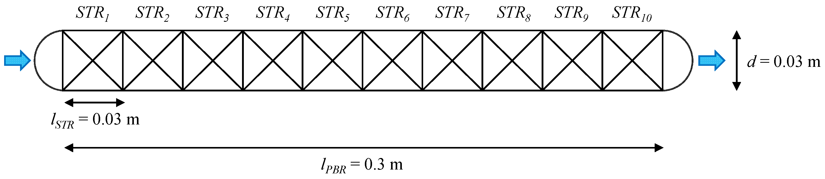
3.2.2. DT Core Model for Enzymatic Hydrolysis Processes in a PBR

Using the new software tool concept, a DT core model for enzymatic hydrolysis processes in a PBR was created to demonstrate that the conditions in a PBR can be modelled by combining a series of STRs. In the STR models, a model representing immobilised biocatalysts was included. The biokinetic and physico-chemical submodels implemented in the STRs correspond to those of the DT for enzymatic hydrolysis processes in a STR [30]. Models for enzymatic starch hydrolysis and proteolysis are forming the biokinetic submodel of the DT. In starch hydrolysis, the substrate starch is converted into glucose by α- and glucoamylases [30]. In proteolysis, proteins are the substrates that are cleaved into free amino acids (products) by endo- and exopeptidases [30]. The physico-chemical submodel is formed by models calculating the temperature and pH of the broth in the reactor.

The DT core model can map the enzymatic hydrolysis processes in a PBR with a length (l_PBR) of 0.3 m, a diameter (d_PBR) of 0.03 m and a volume (V_PBR) of 0.212 L. To reflect the conditions in the PBR, a cascade of ten modified STRs (l_STR = 0.03 m, d_STR = 0.03 m, V_STR = 0.0212 L) was created in the reactor submodel (Figure 7).

The enzymes are immobilised on a carrier substance that is retained in the individual STRs. The ideally mixed substrate solution passes through the STRs from one end of the reactor to the other. In addition, back mixing between the individual STRs can be simulated to represent different flow types.

Figure 8a shows how the product concentration in a simulated proteolysis process in the PBR changes over the length of the reactor from STR₁ to STR₁₀.

It can be seen how the product concentration increases over the length of the PBR from STR₁ (5 g L⁻¹) to STR₁₀ (44 g L⁻¹). After about 45 min, almost stationary conditions are reached in the PBR.

Using the developed DT, a scenario for the combined starch hydrolysis and proteolysis was simulated. The substrate solution containing 100 g L⁻¹ soluble maise starch (80% hydrolysable components) and 100 g L⁻¹ sunflower protein powder (50% hydrolysable components) continuously passed through the PBR (Figure 8b).

For the simulation of the starch hydrolysis process, it can be seen that after the start-up phase of approx. 45 min, the concentration of the substrate rises to approx. 39 g L^−1, and the product concentration rises to approx. 68 g L⁻¹. During the processing time of 20 h, the concentration of active enzyme 1 decreases from 0.08 to 0.079 g L⁻¹, and the concentration of active enzyme 2 decreases from 0.3 to 0.29 g L⁻¹ due to enzyme denaturation. This effect can also be recognised in the concentrations of substrate and product. The substrate concentration increases to approx. 40 g L⁻¹, and the product concentration decreases to 67 g L⁻¹ towards the end of the process.

For the simulation of the proteolysis process, it can be seen that after the start-up phase of approx. 45 min, the concentration of the substrate rises to approx. 56 g L⁻¹, and the product concentration rises to approx. 44 g L⁻¹. During a processing time of 20 h, the concentration of active enzyme 1 decreases from 0.6 to 0.55 g L⁻¹, and the concentration of active enzyme 2 decreases from 0.5 to 0.46 g L⁻¹ due to enzyme denaturation. This effect can also be recognised in the concentrations of substrate and product. The substrate concentration increases up to approx. 59 g L⁻¹, and the product concentration decreases to 41 g L⁻¹ towards the end of the process.

A decrease in enzyme activity affects the conversion of the substrate to the product in starch hydrolysis, as well as in proteolysis. By determining the content of the substrate and product, the enzyme denaturation constant can be identified. With the help of the DT core model, future experiments can be planned in which the enzyme stability can be determined under different process conditions (temperature, pH value).

The new software tool concept enabled the rapid creation of the DT core model for enzymatic hydrolysis processes in a PBR. The desired specifications of the DT core model were entered into the user interface of the new software tool concept. After that, the source code creation of the DT core model took less than one minute, instead of several days if this had to be performed manually. One STR model of this DT core model contains 25 differential equations. The network of ten connected STR models increases the number of differential equations to 250. As the volume in the individual STRs of the PBR does not change, the dilution term in the differential equations for the calculation of the concentrations (see Equations (5) and (6)) could be removed. Since each STR model of the DT core model contains the same biokinetic and physico-chemical submodels, the number of model parameters increases only slightly using ten connected STR models. There are 10 additional parameters describing the exchange area between the STRs. In addition, 20 new control files are added, which specify the flow between the STRs.

Since the newly developed DT core model can map the dynamic behaviour of a PBR approximately, it can serve as a basis for the development of control and automation strategies and thus accelerate the design of a future real process.

4. Conclusions

The new software tool concept enables the rapid and flexible development of bioprocess DT core models. It is possible to create DT core models for various reactor configurations by linking multiple STR models into a network in the reactor submodel. The software tool concept is based on a model library comprising nine different biokinetics with initial parameterisations for a variety of microorganisms and cell lines as well enzymatic systems that can be used as a basis for new biokinetic models. Furthermore, the model library contains five different physico-chemical models that can calculate the most important physico-chemical variables occurring in bioprocesses. In addition, the physico-chemical variables can be predefined with a fixed value or profile. The user can choose the organism, additional enzymatic and biocatalytic reactions and physico-chemical models and create a custom bioprocess DT core model within an hour, compared to several days. This rapid development based on a modular submodel framework also enables faster parameterisations of the developed custom bioprocess DT core models. Submodels can be parameterised independently and sequentially from each other. In the first step, the biokinetic submodel is parameterised with the values of physico-chemical variables as fixed profiles. In the next step, physico-chemical models are added to the DT core model and parameterised. This accelerates parameterisation by at least 90% since time constants in the biokinetic model for microorganisms are generally greater than in the physico-chemical submodel (e.g., temperature model). Despite a user-defined number of STR models, only one biokinetic and one physico-chemical submodel with only one set of parameters are required since the same microorganisms are used in the whole system. The number of connected STR models is only limited by the performance of the PC used for computing.

In the future, the software tool concept for the development of bioprocess DT core models will be continuously upgraded. This includes a systematic expansion of the model library, further options for accelerating the computing time and a further increase in user-friendliness. Using the new software tool concept, the creation and parameterisation of various bioprocess DT core models can be accelerated, and the application possibilities of the DT core models, e.g., for process, control and automation development, can be increased.

References

1. Appl, C.; Moser, A.; Baganz, F.; Hass, V.C. Digital Twins for Bioprocess Control Strategy Development and Realisation. Adv. Biochem. Eng. Biotechnol. 2020, 177, 63–94. [Google Scholar] [CrossRef]
2. Grieves, M. Origins of the Digital Twin Concept; Working Paper; Florida Institute of Technology: Melbourne, FL, USA, 2016. [Google Scholar]
3. Glaessgen, E.; Stargel, D. The Digital Twin Paradigm for Future NASA and U.S. Air Force Vehicles. In Proceedings of the 53rd AIAA/ASME/ASCE/AHS/ASC Structures, Structural Dynamics and Materials Conference, Honolulu, HI, USA, 23–26 April 2012. [Google Scholar] [CrossRef]
4. El Saddik, A. Digital Twins: The Convergence of Multimedia Technologies. IEEE MultiMedia 2018, 25, 87–92. [Google Scholar] [CrossRef]
5. He, R.; Chen, G.; Dong, C.; Sun, S.; Shen, X. Data-driven digital twin technology for optimized control in process systems. ISA Trans. 2019, 95, 221–234. [Google Scholar] [CrossRef]
6. Zobel-Roos, S.; Schmidt, A.; Mestmäcker, F.; Mouellef, M.; Huter, M.; Uhlenbrock, L.; Kornecki, M.; Lohmann, L.; Ditz, R.; Strube, J. Accelerating Biologics Manufacturing by Modeling or: Is Approval under the QbD and PAT Approaches Demanded by Authorities Acceptable Without a Digital-Twin? Processes 2019, 7, 94. [Google Scholar] [CrossRef]
7. Blesgen, A.; Hass, V.C. Operator Training Simulator for Anaerobic Digestion Processes. IFAC Proc. Vol. 2010, 43, 353–358. [Google Scholar] [CrossRef]
8. Moser, A.; Appl, C.; Brüning, S.; Hass, V.C. Mechanistic Mathematical Models as a Basis for Digital Twins. Adv. Biochem. Eng. Biotechnol. 2020, 176, 133–180. [Google Scholar] [CrossRef]
9. Ingenieurbüro Dr.-Ing.Schoop GmbH. WinErs; Ingenieurbüro Dr.-Ing.Schoop GmbH: Hamburg, Germany, 2018. [Google Scholar]
10. Nagy, Z.K. Model based control of a yeast fermentation bioreactor using optimally designed artificial neural networks. Chem. Eng. J. 2007, 127, 95–109. [Google Scholar] [CrossRef]
11. Chen, L.; Nguang, S.K.; Chen, X.D.; Li, X.M. Modelling and optimization of fed-batch fermentation processes using dynamic neural networks and genetic algorithms. Biochem. Eng. J. 2004, 22, 51–61. [Google Scholar] [CrossRef]
12. Grahovac, J.; Jokić, A.; Dodić, J.; Vučurović, D.; Dodić, S. Modelling and prediction of bioethanol production from intermediates and byproduct of sugar beet processing using neural networks. Renew. Energy 2016, 85, 953–958. [Google Scholar] [CrossRef]
13. Konstantinov, K.B.; Yoshida, T. An expert approach for control of fermentation processes as variable structure plants. J. Ferment. Bioeng. 1990, 70, 48–57. [Google Scholar] [CrossRef]
14. Sahakyan, M.; Aung, Z.; Rahwan, T. Explainable Artificial Intelligence for Tabular Data: A Survey. IEEE Access 2021, 9, 135392–135422. [Google Scholar] [CrossRef]
15. Treloar, N.J.; Fedorec, A.J.H.; Ingalls, B.; Barnes, C.P. Deep reinforcement learning for the control of microbial co-cultures in bioreactors. PLoS Comput. Biol. 2020, 16, e1007783. [Google Scholar] [CrossRef] [PubMed]
16. Von Stosch, M.; Davy, S.; Francois, K.; Galvanauskas, V.; Hamelink, J.-M.; Luebbert, A.; Mayer, M.; Oliveira, R.; O’Kennedy, R.; Rice, P.; et al. Hybrid modeling for quality by design and PAT-benefits and challenges of applications in biopharmaceutical industry. Biotechnol. J. 2014, 9, 719–726. [Google Scholar] [CrossRef] [PubMed]
17. Zadeh, L.A. Fuzzy sets. Inf. Control 1965, 8, 338–353. [Google Scholar] [CrossRef]
18. Ying, H. Essentials of fuzzy modeling and control. J. Am. Soc. Inf. Sci. 1995, 46, 791–792. [Google Scholar] [CrossRef]
19. Karakuzu, C.; Türker, M.; Öztürk, S. Modelling, on-line state estimation and fuzzy control of production scale fed-batch baker’s yeast fermentation. Control. Eng. Pract. 2006, 14, 959–974. [Google Scholar] [CrossRef]
20. Horiuchi, J.-I. Fuzzy modeling and control of biological processes. J. Biosci. Bioeng. 2002, 94, 574–578. [Google Scholar] [CrossRef]
21. Monod, J. The Growth of Bacterial Cultures. Annu. Rev. Microbiol. 1949, 3, 371–394. [Google Scholar] [CrossRef]
22. Michaelis, L.; Menten, M.L. Kinetik der Invertinwirkung. Biochem. Ztg. 1913, 49, 333–369. [Google Scholar]
23. Cornish-Bowden, A. One hundred years of Michaelis–Menten kinetics. Perspect. Sci. 2015, 4, 3–9. [Google Scholar] [CrossRef]
24. González-Figueredo, C.; Flores-Estrella, R.A.; Rojas-Rejón, O.A. Fermentation: Metabolism, Kinetic Models, and Bioprocessing. In Current Topics in Biochemical Engineering; Shiomi, N., Ed.; IntechOpen: London, UK, 2019; ISBN 978-1-83881-209-6. [Google Scholar]
25. Craven, S.; Shirsat, N.; Whelan, J.; Glennon, B. Process model comparison and transferability across bioreactor scales and modes of operation for a mammalian cell bioprocess. Biotechnol. Prog. 2013, 29, 186–196. [Google Scholar] [CrossRef] [PubMed]
26. Hodgson, B.J.; Taylor, C.N.; Ushio, M.; Leigh, J.R.; Kalganova, T.; Baganz, F. Intelligent modelling of bioprocesses: A comparison of structured and unstructured approaches. Bioprocess Biosyst. Eng. 2004, 26, 353–359. [Google Scholar] [CrossRef]
27. Esener, A.A.; Roels, J.A.; Kossen, N.W. Theory and applications of unstructured growth models: Kinetic and energetic aspects. Biotechnol. Bioeng. 1983, 25, 2803–2841. [Google Scholar] [CrossRef] [PubMed]
28. Shuler, M.L.; Leung, S.; Dick, C.C. A Mathematical Model for the Growth of a Single Bacterial Cell. Ann. N. Y. Acad. Sci. 1979, 326, 35–52. [Google Scholar] [CrossRef]
29. Nielsen, J.; Nikolajsen, K.; Villadsen, J. Structured modeling of a microbial system: I. A theoretical study of lactic acid fermentation. Biotechnol. Bioeng. 1991, 38, 1–10. [Google Scholar] [CrossRef]
30. Appl, C.; Baganz, F.; Hass, V.C. Development of a Digital Twin for Enzymatic Hydrolysis Processes. Processes 2021, 9, 1734. [Google Scholar] [CrossRef]
31. Brüning, S. Development of a Generalized Process Model for Optimization of Biotechnological Processes. Ph.D. Thesis, Jacobs University, Bremen, Germany, 2016. [Google Scholar]
32. Hass, V.C.; Kuhnen, F.; Schoop, K.-M. An environment for the development of operator training systems (OTS) from chemical engineering models. Comput. Aided Chem. Eng. 2005, 20, 289–293. [Google Scholar] [CrossRef]
33. R Core Team. R Foundation for Statistical Computing; R Core Team: Vienna, Austria, 2014. [Google Scholar]
34. Hirschmann, R. Evaluating the Potential of Anaerobic Production of Ethyl(3)Hydroxybutyrate for Integration in Biorefineries. Ph.D. Thesis, University College London, London, UK, 2022. [Google Scholar]
35. Gerlach, I.; Brüning, S.; Gustavsson, R.; Mandenius, C.-F.; Hass, V.C. Operator training in recombinant protein production using a structured simulator model. J. Biotechnol. 2014, 177, 53–59. [Google Scholar] [CrossRef]
36. Kuntzsch, S. Energy Efficiency Investigations with a New Operator Training Simulator for Biorefineries. Ph.D. Thesis, Jacobs University, Bremen, Germany, 2014. [Google Scholar]
37. Laurí, D.; Lennox, B.; Camacho, J. Model predictive control for batch processes: Ensuring validity of predictions. J. Process. Control. 2014, 24, 239–249. [Google Scholar] [CrossRef]
38. Mears, L.; Stocks, S.M.; Sin, G.; Gernaey, K.V. A review of control strategies for manipulating the feed rate in fed-batch fermentation processes. J. Biotechnol. 2017, 245, 34–46. [Google Scholar] [CrossRef]
39. Moser, A.; Kuchemüller, K.B.; Deppe, S.; Hernández Rodríguez, T.; Frahm, B.; Pörtner, R.; Hass, V.C.; Möller, J. Model-assisted DoE software: Optimization of growth and biocatalysis in Saccharomyces cerevisiae bioprocesses. Bioprocess Biosyst. Eng. 2021, 44, 683–700. [Google Scholar] [CrossRef] [PubMed]
40. Mandenius, C.-F.; Brundin, A. Bioprocess optimization using design-of-experiments methodology. Biotechnol. Prog. 2008, 24, 1191–1203. [Google Scholar] [CrossRef]
41. Candioti, L.V.; de Zan, M.M.; Cámara, M.S.; Goicoechea, H.C. Experimental design and multiple response optimization. Using the desirability function in analytical methods development. Talanta 2014, 124, 123–138. [Google Scholar] [CrossRef] [PubMed]
42. Möller, J.; Kuchemüller, K.B.; Steinmetz, T.; Koopmann, K.S.; Pörtner, R. Model-assisted Design of Experiments as a concept for knowledge-based bioprocess development. Bioprocess Biosyst. Eng. 2019, 42, 867–882. [Google Scholar] [CrossRef] [PubMed]
43. Neubauer, P.; Junne, S. Scale-down simulators for metabolic analysis of large-scale bioprocesses. Curr. Opin. Biotechnol. 2010, 21, 114–121. [Google Scholar] [CrossRef] [PubMed]
44. Oosterhuis, N.M.; Kossen, N.W. Dissolved oxygen concentration profiles in a production-scale bioreactor. Biotechnol. Bioeng. 1984, 26, 546–550. [Google Scholar] [CrossRef]
45. Hewitt, C.J.; Nienow, A.W. The scale-up of microbial batch and fed-batch fermentation processes. Adv. Appl. Microbiol. 2007, 62, 105–135. [Google Scholar] [CrossRef]
46. Enfors, S.O.; Jahic, M.; Rozkov, A.; Xu, B.; Hecker, M.; Jürgen, B.; Krüger, E.; Schweder, T.; Hamer, G.; O’Beirne, D.; et al. Physiological responses to mixing in large scale bioreactors. J. Biotechnol. 2001, 85, 175–185. [Google Scholar] [CrossRef]
47. George, S.; Larsson, G.; Olsson, K.; Enfors, S.-O. Comparison of the Baker’s yeast process performance in laboratory and production scale. Bioprocess Eng. 1998, 18, 135–142. [Google Scholar] [CrossRef]
48. Larsson, G.; Trnkvist, M.; Wernersson, E.S.; Trgrdh, C.; Noorman, H.; Enfors, S.-O. Substrate gradients in bioreactors: Origin and consequences. Bioprocess Eng. 1996, 14, 281–289. [Google Scholar] [CrossRef]
49. Formenti, L.R.; Nørregaard, A.; Bolic, A.; Hernandez, D.Q.; Hagemann, T.; Heins, A.-L.; Larsson, H.; Mears, L.; Mauricio-Iglesias, M.; Krühne, U.; et al. Challenges in industrial fermentation technology research. Biotechnol. J. 2014, 9, 727–738. [Google Scholar] [CrossRef] [PubMed]
50. Sweere, A.P.J.; Matla, Y.A.; Zandvliet, J.; Luyben, K.C.A.M.; Kossen, N.W.F. Experimental simulation of glucose fluctuations. Appl. Microbiol. Biotechnol. 1988, 28, 109–115. [Google Scholar] [CrossRef]
51. Sandoval-Basurto, E.A.; Gosset, G.; Bolívar, F.; Ramírez, O.T. Culture of Escherichia coli under dissolved oxygen gradients simulated in a two-compartment scale-down system: Metabolic response and production of recombinant protein. Biotechnol. Bioeng. 2005, 89, 453–463. [Google Scholar] [CrossRef] [PubMed]
52. Lara, A.R.; Galindo, E.; Ramírez, O.T.; Palomares, L.A. Living with heterogeneities in bioreactors: Understanding the effects of environmental gradients on cells. Mol. Biotechnol. 2006, 34, 355–381. [Google Scholar] [CrossRef]
53. Fiechter, A.; Fuhrmann, G.F.; Käppeli, O. Regulation of Glucose Metabolism in Growing Yeast Cells. Adv. Microb. Physiol. 1981, 22, 123–183. [Google Scholar] [CrossRef]
54. Sonnleitner, B.; Käppeli, O. Growth of Saccharomyces cerevisiae is controlled by its limited respiratory capacity: Formulation and verification of a hypothesis. Biotechnol. Bioeng. 1986, 28, 927–937. [Google Scholar] [CrossRef]
55. Bai, F.W.; Anderson, W.A.; Moo-Young, M. Ethanol fermentation technologies from sugar and starch feedstocks. Biotechnol. Adv. 2008, 26, 89–105. [Google Scholar] [CrossRef]
56. Larsson, C.; von Stockar, U.; Marison, I.; Gustafsson, L. Growth and Metabolism of Saccharomyces cerevisiae in Chemostat Cultures under Carbon-, Nitrogen-, or Carbon- and Nitrogen-Limiting Conditions. J. Bacteriol. 1993, 175, 4809–4816. [Google Scholar] [CrossRef]
57. Nelder, J.A.; Mead, R. A Simplex Method for Function Minimization. Comput. J. 1965, 7, 308–313. [Google Scholar] [CrossRef]
58. Nienow, A.W. Scale-Up, Stirred Tank Reactors. In Encyclopedia of Industrial Biotechnology: Bioprocess, Bioseparation, and Cell Technology; John Wiley & Sons, Inc.: Hoboken, NJ, USA, 2010; pp. 1–38. [Google Scholar] [CrossRef]
59. Van’t Riet, K.; Tramper, J. Basic Bioreactor Design, 1st ed.; CRC Press: Boca Raton, FL, USA, 1991; ISBN 9781482293333. [Google Scholar]
Figure 1. Shell structure for bioprocess DTs based on [7,8]. Extended by definitions for DT core model, digital control test simulator and detached DT.
Fermentation 10 00463 g001
Figure 2. Software tool concept for the rapid development of mechanistic DT core models for bioprocesses in various reactor designs.
Fermentation 10 00463 g002
Figure 3. Combination of the DT submodels to enable the simulation of various reactor designs, (a) mass transfer flows between STR models, and (b) individually adjustable inputs and outputs.
Fermentation 10 00463 g003
Figure 4. DT reactor configurations that can be created with the new software tool concept. Each green-dotted box indicates one individual STR model.
Fermentation 10 00463 g004
Figure 5. DT for the cultivation of S. cerevisiae in two connected parallel ideal STRs. Blue arrows symbolise the flow between the ideal STR models (green dotted boxes).
Fermentation 10 00463 g005
Figure 6. Experimental data in comparison to simulation results using the DT for the system of two interconnected 1 L STRs. (a) shows the concentrations of glucose (red, circle), ethanol (blue, square) and the dry cell weight (DCW, green, triangle) in R1. (b) shows the online data of the exhaust gas concentration of O2 (simulated = dark red, experimental = light red) and CO2 (simulated = black, experimental = grey) of R1 and R2. (c) shows the pH (simulated = dark red, experimental = light red), the feed rate of the glucose medium (500 g L−1 glucose) and the simulated volume of the reactor medium of both reactors (R1 = black, R2 = grey).
Fermentation 10 00463 g006
Figure 7. DT for enzymatic hydrolysis processes in a PBR (ten connected STRs) with immobilised enzymes. Blue arrows symbolise the flow direction of nutrient media through the PBR.
Fermentation 10 00463 g007
Figure 8. DT simulation of the combined enzymatic starch hydrolysis (SH) and proteolysis (PR) in ten STRs representing a PBR (l = 0.3 m, d = 0.03 m) with T = 60 °C, pH = 6, inflow of substrate solution = 10 mL min−1 (100 g L−1 substrate SH (80% hydrolysable), 100 g L−1 substrate PR (50% hydrolysable)), back mixing = 1 mL min−1; (a) proteolysis start-up phase in the STRs 1–10 with P: product (free amino acids) concentration; (b) continuous process over 20 h with S: substrate concentration, P: product concentration, E1: active α-amylase (SH) or endopeptidase (PR) concentration, E2: active glucoamylase concentration (SH) exopeptidase (PR).
Fermentation 10 00463 g008