
Evaluation of Environmental Sustainability of Biorefinery and Incineration with Energy Recovery Based on Life Cycle Assessment †

Abstract
:1. Introduction
2. Materials and Methods
2.1. Experimental Design
2.1.1. Goal, Scope, System Description, and Limitations in the LCA of the BRF and IER
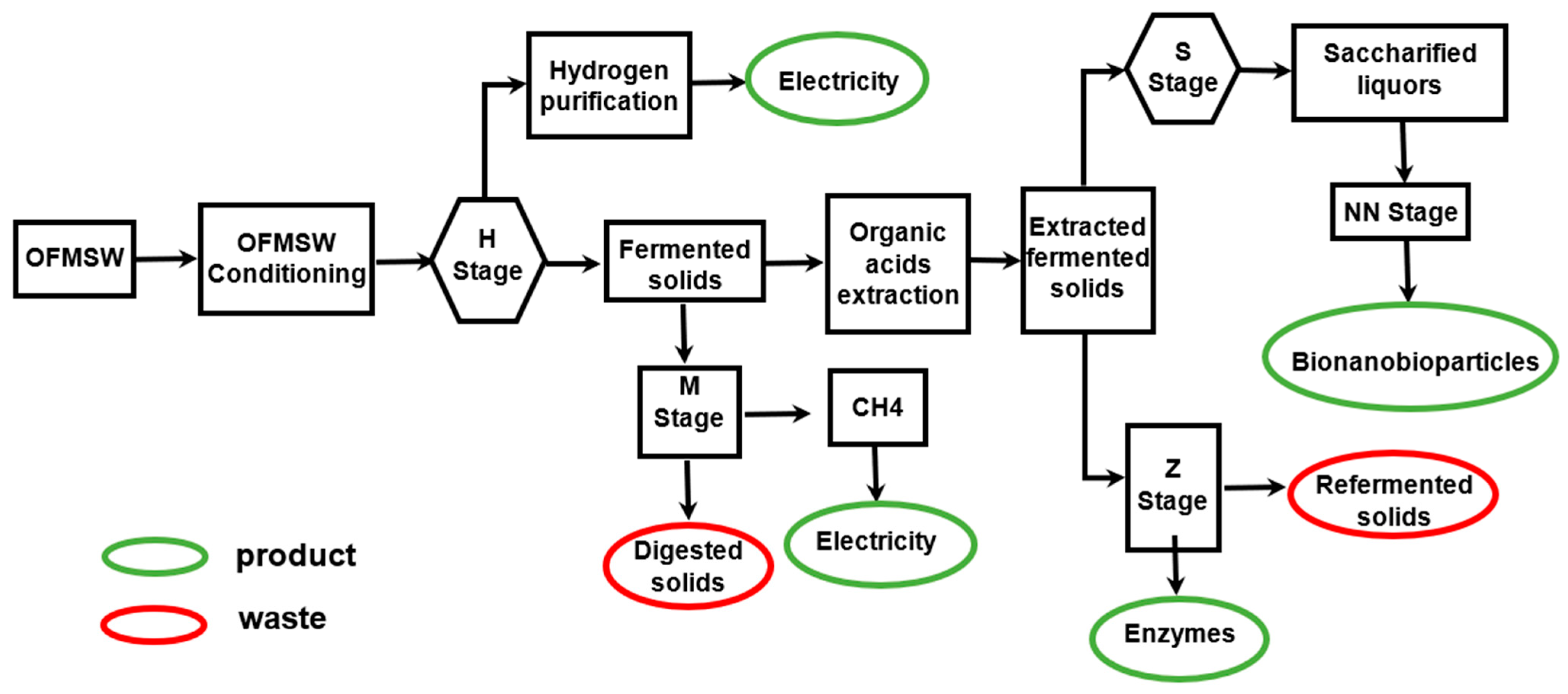
Biorefinery HMEZS-NN
Incineration with Energy Recovery
2.1.2. Life Cycle Inventory
2.1.3. Environmental Impact Assessment
2.1.4. Interpretation of Results
2.2. Comparison of Environmental Impacts and Sustainability of the Biorefinery and Incineration in Our Work
3. Results and Discussion
3.1. Energy Performance of the Biorefinery and Incineration in This Work
3.2. Environmental Performance of the Biorefinery
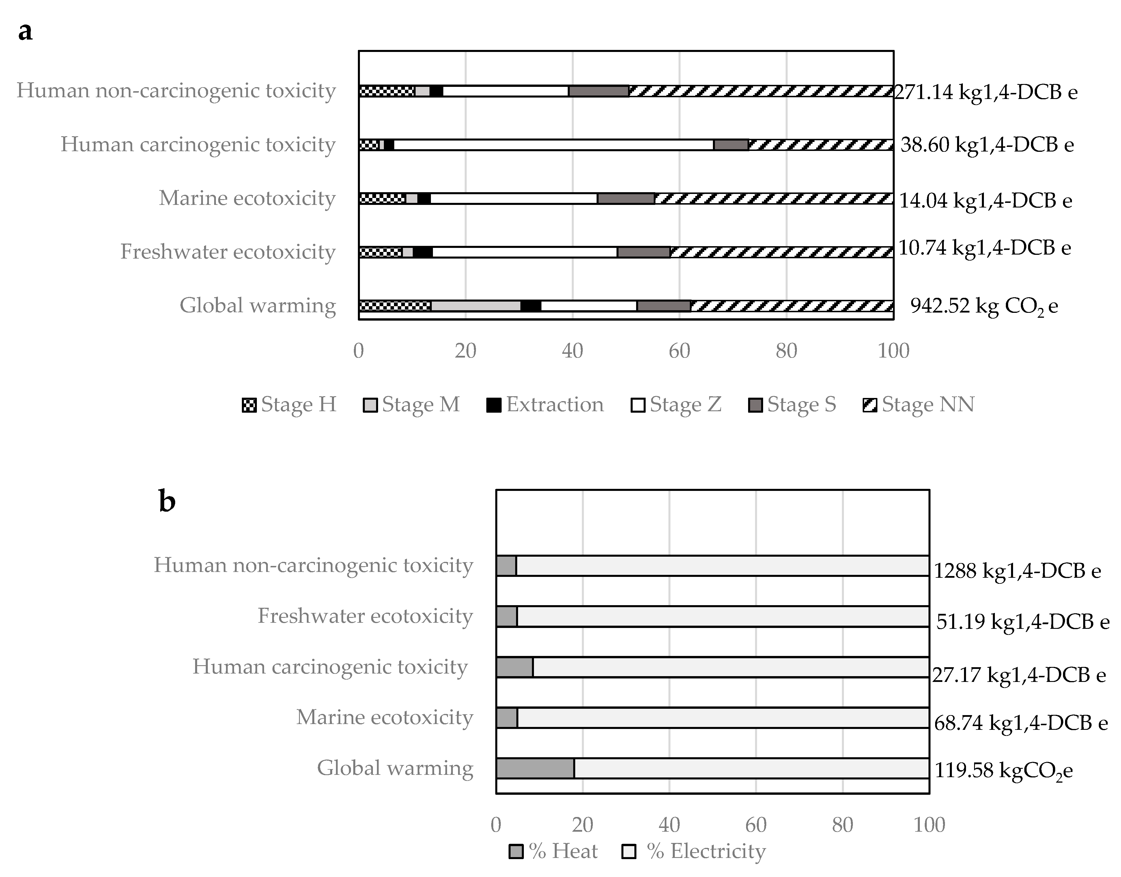
3.2.1. Environmental Impact Description and Contributions
3.2.2. Comparison with Reported Cases of Biorefineries
“Biorefineries could be described as integrated bio-based industries that use a variety of technologies to produce products such as chemicals, biofuels, food and feed ingredients, biomaterials, fibers, and heat and power, with the aim of maximizing added value along the three pillars of sustainability (environment, economy, and society)”.
3.3. Environmental Performance of Incineration with Energy Recovery
3.3.1. Description of Environmental Impacts and Contributions
3.3.2. Comparison with Reported Incineration Cases
3.4. Comparison of the Global Environmental Sustainability of the Biorefinery and Incineration in This Work
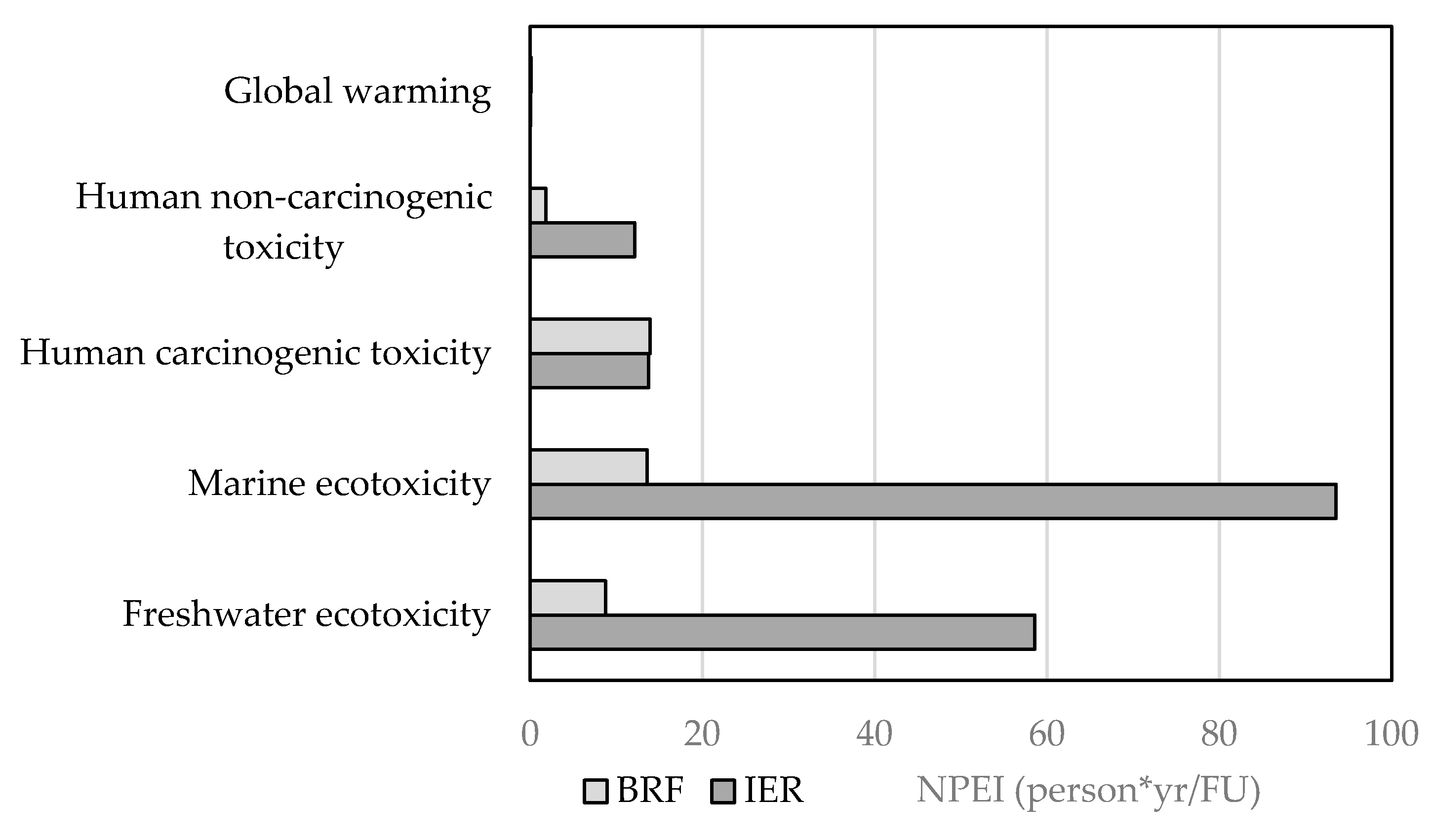
3.4.1. Comparison of Environmental Sustainability
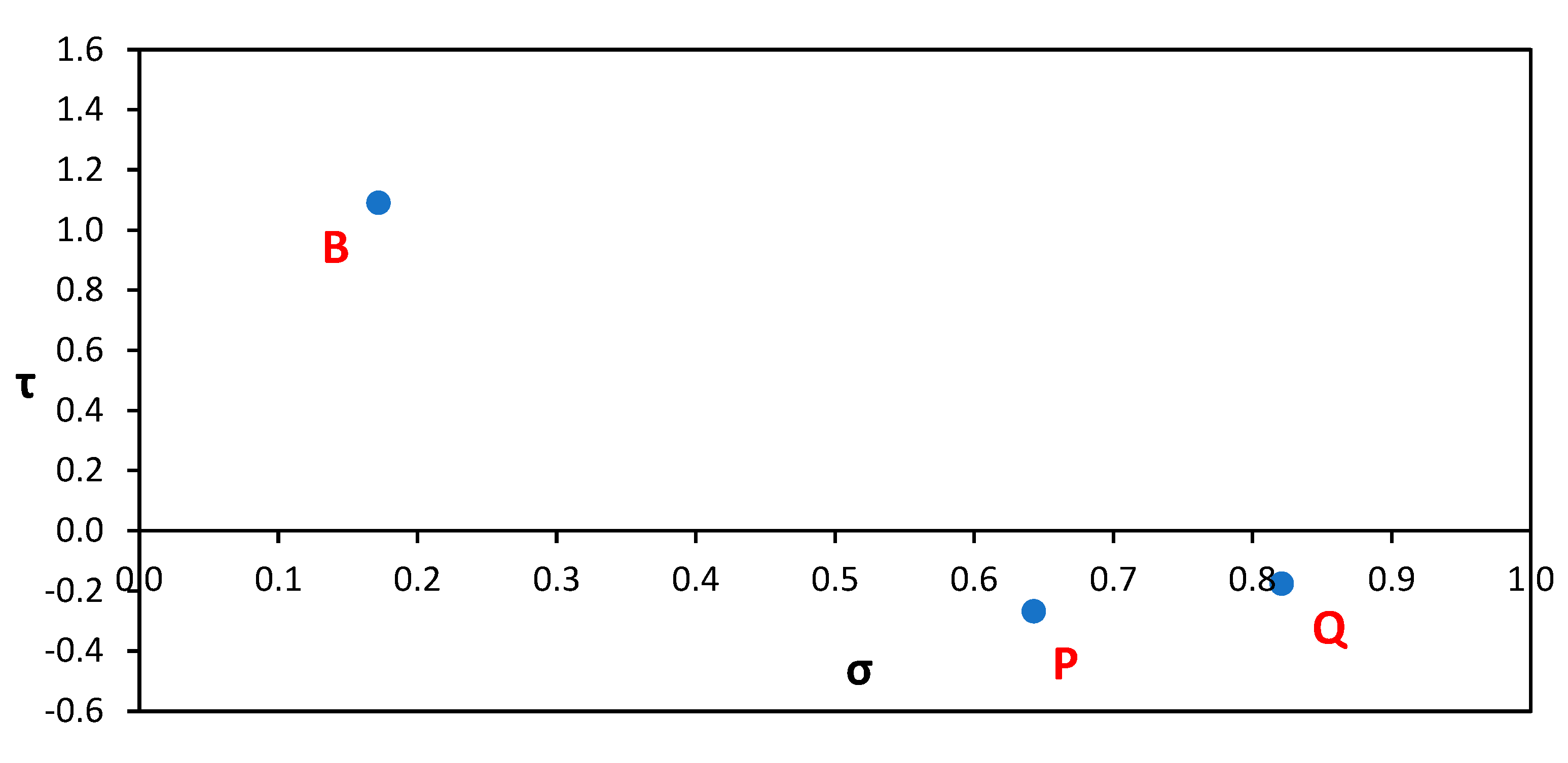
3.4.2. Sensitivity Tests
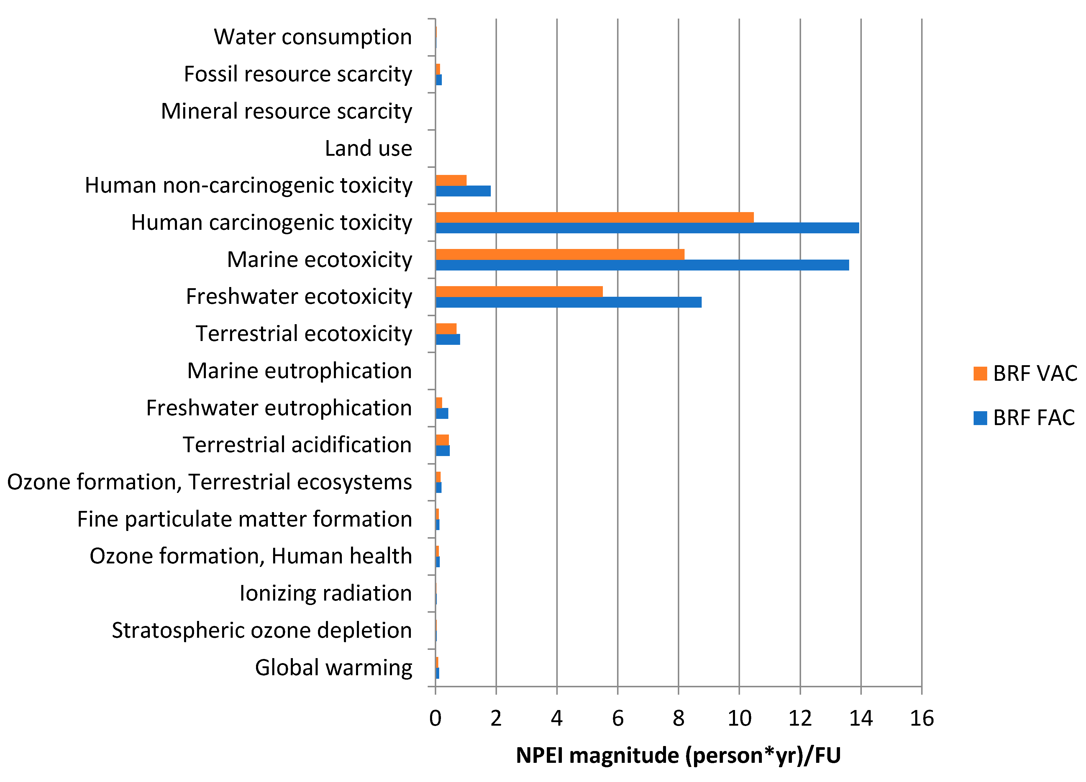
Sensitivity of Biorefinery Environmental Sustainability to Changes in the Type of Activated Carbon Used in the NN Stage of the Biorefinery
Sensitivity of Indicators and Environmental Sustainability to Weighting
4. Conclusions
Supplementary Materials
Author Contributions
Funding
Institutional Review Board Statement
Informed Consent Statement
Data Availability Statement
Acknowledgments
Conflicts of Interest
Nomenclature
| BNBP | Bionanobioparticle |
| BRF | Biorefinery |
| DeNOx | system treatment of gas emissions that remove nitrogen oxides from flue gas in IER |
| DC | developed country |
| DCBe | dichlorobenzene equivalent |
| E | extraction of organic acids and solvents, a stage of the BRF biorefinery |
| EfW | energy from waste |
| ES | environmental sustainability |
| ESP | electrostatic fly ash precipitator |
| Fcorrection | correction factor to standardize to USD January 2025, given that the cost data were usually reported in different years |
| FGWS | flue gas wet scrubber |
| FGT | flue gas treatment |
| FLUWA | acid leaching of ashes |
| Fn | factor of normalization, used to calculate the NPEI from PEI (potential environmental impact) |
| FP | fine particle |
| FRS | fossil resource scarcity |
| FWEc | freshwater ecotoxicity |
| FWEu | freshwater eutrophication |
| FU | functional unit |
| FW | fermented waste |
| GHG | greenhouse gas effect |
| GBAER | Environmental Biotechnology and Renewable Energies Group |
| GW | global warming |
| H | Hydrogen |
| H2Succ | succinic acid |
| HCT | human carcinogenic toxicity |
| HNCT | human non-carcinogenic toxicity |
| HT | human toxicity |
| IER | incineration with energy recovery |
| IR | ionizing radiation |
| LCA | Life Cycle Assessment |
| LCI | life cycle inventory |
| LF | landfill or landfilling |
| LU | land use |
| MEc | marine ecotoxicity |
| Meu | marine eutrophication |
| M | Methane |
| MRS | mineral resource scarcity |
| MSW | municipal solid waste |
| NN | bionanobioparticle stage |
| NSCR | non-selective catalytic reduction |
| NPEI | normalized potential environmental impact |
| NSCR | non-selective catalytic reduction |
| OFH | ozone formation, human health |
| OFMSW | organic fraction of municipal solid waste |
| OFTE | ozone formation terrestrial ecosystem |
| PEI | potential environmental impact |
| PET | Terephthalate-polyethylene |
| PHA | Polyhydroxyalkanoate |
| POI | photochemical ozone impact |
| S | stage in the BRF that produces saccharified liquors |
| SMR | scarcity of mineral resources |
| SOD | stratospheric ozone depletion |
| SCR | selective catalytic reduction |
| SM | Supplementary Materials |
| TA | terrestrial acidification |
| TE | terrestrial ecotoxicity |
| TIC | total investment cost |
| TS | total solid |
| U | unit load of environmental impact per person and per year (units of characterization impact/(person*yr)) |
| U | overall heat transfer coefficient in heat transfer equations |
| UC | underdeveloped country |
| UOW | urban organic waste |
| VAPs | value-added products |
| VOA | volatile organic (fatty) acid |
| WC | water consumption |
| Z | stage in the BRF that produces a concentrate of industrial enzymes |
| Greek characters | |
| α | alpha (in) sustainability index Equation (A8.1), unit (person*yr)/FU |
| γ | specific investment cost, in USD/t waste or biomass fed |
| Γ | Capacity |
| δ | correction for the different dry matter contents in Equation (4) |
| ∆μ | indicates the percent increase in the maximum value of impact in one technology compared to the minimum value of the same impact in the other technology, as defined by Equation (2) |
| µ | ratio that indicates which technology is more contaminant in a given category ‘j’ of environmental impact Equation (1) (%) |
| Φ | correction for different reference flows Equation (1) |
| φ(X) | units of the magnitude X enclosed in the brackets, for typical potential environmental impacts in Equation (2) |
| σ | sigma sustainability index in Equation (A8.2), dimensionless |
| ꚍ | tau sustainability index in Equation (A8.3), dimensionless |
References
- Kaza, S.; Yao, L.C.; Bhada-Tata, P.; Van Woerden, F. What a Waste 2.0: A Global Snapshot of Solid Waste Management to 2050; World Bank Group: Washington, DC, USA, 2018. [Google Scholar] [CrossRef]
- Botello-Álvarez, J.E.; Rivas-García, P.; Fausto-Castro, L.; Estrada-Baltazar, A.; Gomez-Gonzalez, R. Informal Collection, Recycling and Export of Valuable Waste as Transcendent Factor in the Municipal Solid Waste Management: A Latin-American Reality. J. Clean Prod. 2018, 182, 485–495. [Google Scholar] [CrossRef]
- Mor, S.; Ravindra, K. Municipal Solid Waste Landfills in Lower- and Middle-Income Countries: Environmental Impacts, Challenges and Sustainable Management Practices. Process Saf. Environ. Prot. 2023, 174, 510–530. [Google Scholar] [CrossRef]
- Semarnat. Diagnóstico Básico para la Gestión Integral de los Residuos; Secretaría de Medio Ambiente y Recursos Naturales: México City, Mexico, 2020. [Google Scholar]
- INECC. Inventario Nacional de Emisiones de Gases y Compuestos de Efecto Invernadero. Instituto Nacional de Ecología y Cambio Climático. Available online: https://www.gob.mx/inecc/acciones-y-programas/inventario-nacional-de-emisiones-de-gases-y-compuestos-de-efecto-invernadero (accessed on 23 June 2024).
- Nath, A.; Debnath, A. A Short Review on Landfill Leachate Treatment Technologies. Mater. Today Proc. 2022, 67, 1290–1297. [Google Scholar] [CrossRef]
- Renou, S.; Givaudan, J.G.; Poulain, S.; Dirassouyan, F.; Moulin, P. Landfill Leachate Treatment: Review and Opportunity. J. Hazard. Mater. 2008, 150, 468–493. [Google Scholar] [CrossRef]
- Luo, H.; Zeng, Y.; Cheng, Y.; He, D.; Pan, X. Recent Advances in Municipal Landfill Leachate: A Review Focusing on Its Characteristics, Treatment, and Toxicity Assessment. Sci. Total Environ. 2020, 703, 135468. [Google Scholar] [CrossRef]
- Coelho, S.T.; Diaz-Chavez, R. Best Available Technologies (BAT) for WtE in Developing Countries. In Municipal Solid Waste Energy Conversion in Developing Countries: Technologies, Best Practices, Challenges and Policy; Elsevier: Amsterdam, The Netherlands, 2020; pp. 63–105. [Google Scholar] [CrossRef]
- Khan, M.S.; Mubeen, I.; Caimeng, Y.; Zhu, G.; Khalid, A.; Yan, M. Waste to Energy Incineration Technology: Recent Development under Climate Change Scenarios. Waste Manag. Res. J. Sustain. Circ. Econ. 2022, 40, 1708–1729. [Google Scholar] [CrossRef]
- Kissas, K.; Ibrom, A.; Kjeldsen, P.; Scheutz, C. Methane Emission Dynamics from a Danish Landfill: The Effect of Changes in Barometric Pressure. Waste Manag. 2022, 138, 234–242. [Google Scholar] [CrossRef]
- Sisani, F.; Maalouf, A.; Di Maria, F. Environmental and Energy Performances of the Italian Municipal Solid Waste Incineration System in a Life Cycle Perspective. Waste Manag. Res. J. Sustain. Circ. Econ. 2022, 40, 218–226. [Google Scholar] [CrossRef]
- Escamilla-García, P.E.; Camarillo-López, R.H.; Carrasco-Hernández, R.; Fernández-Rodríguez, E.; Legal-Hernández, J.M. Technical and Economic Analysis of Energy Generation from Waste Incineration in Mexico. Energy Strategy Rev. 2020, 31, 100542. [Google Scholar] [CrossRef]
- ENRES. Potencial para la Valorización Energética de Residuos Urbanos en México, a Través Del Coprocesamiento en Hornos Cementeros; GIZ: México City, Mexico; SENER: México City, Mexico; SEMARNAT: México City, Mexico, 2016. [Google Scholar]
- Faragó, T.; Špirová, V.; Blažeková, P.; Lalinská-Voleková, B.; Macek, J.; Jurkovič, Ľ.; Vítková, M.; Hiller, E. Environmental and Health Impacts Assessment of Long-Term Naturally-Weathered Municipal Solid Waste Incineration Ashes Deposited in Soil—Old Burden in Bratislava City, Slovakia. Heliyon 2023, 9, e13605. [Google Scholar] [CrossRef]
- Monni, S. From Landfilling to Waste Incineration: Implications on GHG Emissions of Different Actors. Int. J. Greenh. Gas Control. 2012, 8, 82–89. [Google Scholar] [CrossRef]
- Zhu, Y.; Hu, Y.; Guo, Q.; Zhao, L.; Li, L.; Wang, Y.; Hu, G.; Wibowo, H.; Di Maio, F. The Effect of Wet Treatment on the Distribution and Leaching of Heavy Metals and Salts of Bottom Ash from Municipal Solid Waste Incineration. Environ. Eng. Sci. 2022, 39, 409–417. [Google Scholar] [CrossRef]
- Duan, Y.; Tarafdar, A.; Kumar, V.; Ganeshan, P.; Rajendran, K.; Shekhar Giri, B.; Gómez-García, R.; Li, H.; Zhang, Z.; Sindhu, R.; et al. Sustainable Biorefinery Approaches towards Circular Economy for Conversion of Biowaste to Value Added Materials and Future Perspectives. Fuel 2022, 325, 124846. [Google Scholar] [CrossRef]
- Khoshnevisan, B.; Duan, N.; Tsapekos, P.; Awasthi, M.K.; Liu, Z.; Mohammadi, A.; Angelidaki, I.; Tsang, D.C.W.; Zhang, Z.; Pan, J.; et al. A Critical Review on Livestock Manure Biorefinery Technologies: Sustainability, Challenges, and Future Perspectives. Renew. Sustain. Energy Rev. 2021, 135, 110033. [Google Scholar] [CrossRef]
- Ladakis, D.; Stylianou, E.; Ioannidou, S.M.; Koutinas, A.; Pateraki, C. Biorefinery Development, Techno-Economic Evaluation and Environmental Impact Analysis for the Conversion of the Organic Fraction of Municipal Solid Waste into Succinic Acid and Value-Added Fractions. Bioresour. Technol. 2022, 354, 127172. [Google Scholar] [CrossRef]
- Lopes da Silva, T.; Fontes, A.; Reis, A.; Siva, C.; Gírio, F. Oleaginous Yeast Biorefinery: Feedstocks, Processes, Techniques, Bioproducts. Fermentation 2023, 9, 1013. [Google Scholar] [CrossRef]
- Shah, A.V.; Singh, A.; Sabyasachi Mohanty, S.; Kumar Srivastava, V.; Varjani, S. Organic Solid Waste: Biorefinery Approach as a Sustainable Strategy in Circular Bioeconomy. Bioresour. Technol. 2022, 349, 126835. [Google Scholar] [CrossRef]
- Escamilla-Alvarado, C.; Poggi-Varaldo, H.M.; Ponce-Noyola, M.T. Bioenergy and Bioproducts from Municipal Organic Waste as Alternative to Landfilling: A Comparative Life Cycle Assessment with Prospective Application to Mexico. Environ. Sci. Pollut. Res. 2017, 24, 25602–25617. [Google Scholar] [CrossRef]
- Fava, F.; Totaro, G.; Diels, L.; Reis, M.; Duarte, J.; Carioca, O.B.; Poggi-Varaldo, H.M.; Ferreira, B.S. Biowaste Biorefinery in Europe: Opportunities and Research & Development Needs. New Biotechnol. 2015, 32, 100–108. [Google Scholar] [CrossRef]
- Kirtay, E. Recent Advances in Production of Hydrogen from Biomass. Energy Convers. Manag. 2011, 52, 1778–1789. [Google Scholar] [CrossRef]
- Poggi-Varaldo, H.M.; Munoz-Paez, K.M.; Escamilla-Alvarado, C.; Robledo-Narváez, P.N.; Ponce-Noyola, M.T.; Calva-Calva, G.; Ríos-Leal, E.; Galíndez-Mayer, J.; Estrada-Vázquez, C.; Ortega-Clemente, A.; et al. Biohydrogen, Biomethane and Bioelectricity as Crucial Components of Biorefinery of Organic Wastes: A Review. Waste Manag. Res. 2014, 32, 353–365. [Google Scholar] [CrossRef] [PubMed]
- Gottardo, M.; Dosta, J.; Cavinato, C.; Crognale, S.; Tonanzi, B.; Rossetti, S.; Bolzonella, D.; Pavan, P.; Valentino, F. Boosting Butyrate and Hydrogen Production in Acidogenic Fermentation of Food Waste and Sewage Sludge Mixture: A Pilot Scale Demonstration. J. Clean. Prod. 2023, 404, 136919. [Google Scholar] [CrossRef]
- Hernández-Correa, E.; Poggi-Varaldo, H.M.; Ponce-Noyola, M.T.; Romero-Cedillo, L.; Ríos-Leal, E.; Solorza-Feria, O. Production of Value-Added Products and Commodities by Electrofermentation and Its Integration to Biorefineries. In Proceedings of the Fourth International Symposium on Bioremediation and Sustainable Environmental Technologies, Miami, FL, USA, 22 May 2017; Available online: https://www.battelle.org/docs/default-source/conferences/bioremediation-symposium/proceedings/biosymposium/innovative-biological-approaches-to-pollution-prevention-and-waste-management/c6_-580_ppr.pdf?sfvrsn=88efb388_0 (accessed on 29 November 2024).
- International Energy Agency. Global Biorefinery Status Report 2022|Task42. 2022. Available online: https://task42.ieabioenergy.com/publications/global-biorefinery-status-report-2022/ (accessed on 23 July 2024).
- U.S. Energy Information Administration. International Energy Outlook 2023; U.S. Energy Information Administration: Washington, DC, USA, 2023. [Google Scholar]
- Secretaría de Medio Ambiente y Recursos Naturales. SEMARNAT Apoya Gestión de Residuos Través de Plantas de Termovalorización. Available online: https://www.gob.mx/semarnat/prensa/semarnat-apoya-gestion-de-residuos-a-traves-de-plantas-de-termovalorizacion (accessed on 5 November 2024).
- United Nations Environment Programme. Waste-to-Energy: Considerations for Informed Decision-Making. 2019. Available online: http://wedocs.unep.org/bitstream/handle/20.500.11822/28413/WTEfull.pdf?sequence%E2%80%A6 (accessed on 31 July 2024).
- Makepa, D.C.; Chihobo, C.H. Barriers to Commercial Deployment of Biorefineries: A Multi-Faceted Review of Obstacles across the Innovation Chain. Heliyon 2024, 10, e32649. [Google Scholar] [CrossRef]
- Sacramento-Rivero, J.; Navarro-Pineda, F. Evaluación de La Sostenibilidad Para El Diseño Conceptual de Biorrefinerías. In Biorrefinerías y Economía Circular; Carrillo-Gozález, G., Torres-Bustillos Luis, G., Eds.; Universidad Autónoma Metropolitana: Mexico City, Mexico, 2019; pp. 121–146. [Google Scholar]
- Yáñez Vergara, A.G.; Sotelo-Navarro, P.X.; Poggi-Varaldo, H.M.; Calderón-Salinas, J.V.; Sánchez-Pérez, R.; Matsumoto-Kuwahara, Y. Análisis de Legislación Sobre Biorrefinerías En México. Rev. Int. Contam. Ambient. 2022, 38, 111–142. [Google Scholar] [CrossRef]
- Lino, F.A.M.; Ismail, K.A.R. Evaluation of the Treatment of Municipal Solid Waste as Renewable Energy Resource in Campinas, Brazil. Sustain. Energy Technol. Assess. 2018, 29, 19–25. [Google Scholar] [CrossRef]
- Mia, S.; Uddin, M.E.; Kader, M.A.; Ahsan, A.; Mannan, M.A.; Hossain, M.M.; Solaiman, Z.M. Pyrolysis and Co-Composting of Municipal Organic Waste in Bangladesh: A Quantitative Estimate of Recyclable Nutrients, Greenhouse Gas Emissions, and Economic Benefits. Waste Manag. 2018, 75, 503–513. [Google Scholar] [CrossRef]
- Starostina, V.; Damgaard, A.; Eriksen, M.K.; Christensen, T.H. Waste Management in the Irkutsk Region, Siberia, Russia: An Environmental Assessment of Alternative Development Scenarios. Waste Manag. Res. J. Sustain. Circ. Econ. 2018, 36, 373–385. [Google Scholar] [CrossRef]
- Gupta, N.; Yadav, K.K.; Kumar, V. A Review on Current Status of Municipal Solid Waste Management in India. J. Environ. Sci. 2015, 37, 206–217. [Google Scholar] [CrossRef]
- Mudofir, M.; Astuti, S.P.; Purnasari, N.; Sabariyanto, S.; Yenneti, K.; Ogan, D.D. Waste harvesting: Lessons learned from the development of waste-to-energy power plants in Indonesia. Int. J. Energy Sect. Manag. 2025. [Google Scholar] [CrossRef]
- Tonini, D.; Astrup, T. Life-Cycle Assessment of a Waste Refinery Process for Enzymatic Treatment of Municipal Solid Waste. Waste Manag. 2012, 32, 165–176. [Google Scholar] [CrossRef]
- Ma, H.; Wei, Y.; Fei, F.; Gao, M.; Wang, Q. Whether Biorefinery Is a Promising Way to Support Waste Source Separation? From the Life Cycle Perspective. Sci. Total Environ. 2024, 912, 168731. [Google Scholar] [CrossRef] [PubMed]
- Clasen, A.P.; Agostinho, F.; Sulis, F.; Almeida, C.M.V.B.; Giannetti, B.F. Unlocking the Potential of Municipal Solid Waste: Emergy Accounting Applied in a Novel Biorefinery. Ecol. Modell. 2024, 492, 110725. [Google Scholar] [CrossRef]
- Jing, H.; Wang, H.; Lin, C.S.K.; Zhuang, H.; To, M.H.; Leu, S.-Y. Biorefinery Potential of Chemically Enhanced Primary Treatment Sewage Sludge to Representative Value-Added Chemicals—A de Novo Angle for Wastewater Treatment. Bioresour. Technol. 2021, 339, 125583. [Google Scholar] [CrossRef] [PubMed]
- Teh, K.C.; Tan, J.; Chew, I.M.L. Multiple Biogenic Waste Valorization via Pyrolysis Technologies in Palm Oil Industry: Economic and Environmental Multi-Objective Optimization for Sustainable Energy System. Process Integr. Optim. Sustain. 2023, 7, 847–860. [Google Scholar] [CrossRef]
- Mu, D.; Addy, M.; Anderson, E.; Chen, P.; Ruan, R. A Life Cycle Assessment and Economic Analysis of the Scum-to-Biodiesel Technology in Wastewater Treatment Plants. Bioresour. Technol. 2016, 204, 89–97. [Google Scholar] [CrossRef]
- ISO 14044; Environmental Management—Life Cycle Assessment—Reuirements and Guidelines. The International Organization for Standardization: Geneva, Switzerland, 2006.
- ISO 14040; Environmental Management—Life Cycle Assessment—Principles and Framework. The Internation Organization for Standardization: Geneva, Switzerland, 2006.
- Guo, M.; Murphy, R.J. LCA Data Quality: Sensitivity and Uncertainty Analysis. Sci. Total Environ. 2012, 435–436, 230–243. [Google Scholar] [CrossRef]
- Anshassi, M.; Laux, S.J.; Townsend, T.G. Approaches to Integrate Sustainable Materials Management into Waste Management Planning and Policy. Resour. Conserv. Recycl. 2019, 148, 55–66. [Google Scholar] [CrossRef]
- Dastjerdi, B.; Strezov, V.; Rajaeifar, M.A.; Kumar, R.; Behnia, M. A Systematic Review on Life Cycle Assessment of Different Waste to Energy Valorization Technologies. J. Clean Prod. 2021, 290, 125747. [Google Scholar] [CrossRef]
- Evangelisti, S.; Tagliaferri, C.; Clift, R.; Lettieri, P.; Taylor, R.; Chapman, C. Life Cycle Assessment of Conventional and Two-Stage Advanced Energy-from-Waste Technologies for Municipal Solid Waste Treatment. J. Clean. Prod. 2015, 100, 212–223. [Google Scholar] [CrossRef]
- Cherubini, F.; Bird, N.D.; Cowie, A.; Jungmeier, G.; Schlamadinger, B.; Woess-Gallasch, S. Energy- and Greenhouse Gas-Based LCA of Biofuel and Bioenergy Systems: Key Issues, Ranges and Recommendations. Resour. Conserv. Recycl. 2009, 53, 434–447. [Google Scholar] [CrossRef]
- Tagliaferri, C.; Evangelisti, S.; Clift, R.; Lettieri, P.; Chapman, C.; Taylor, R. Life Cycle Assessment of Conventional and Advanced Two-Stage Energy-from-Waste Technologies for Methane Production. J. Clean. Prod. 2016, 129, 144–158. [Google Scholar] [CrossRef]
- Sotelo-Navarro, P.X.; Poggi-Varaldo, H.M.; Chargoy-Amador, J.P.; Sojo-Benítez, A.; Pérez-Angón, M.Á.; Sánchez-Pérez, R. Environmental Impacts of an HMEZS Biorefinery. Rev. Int. Contam. Ambient. 2022, 38, 48–57. [Google Scholar] [CrossRef]
- Pérez-Morales, G.; Poggi-Varaldo, H.M.; Ponce-Noyola, T.; Pérez-Valdespino, A.; Curiel-Quesada, E.; Galíndez-Mayer, J.; Ruiz-Ordaz, N.; Sotelo-Navarro, P.X. A Review of the Production of Hyaluronic Acid in the Context of Its Integration into GBAER-Type Biorefineries. Fermentation 2024, 10, 305. [Google Scholar] [CrossRef]
- World Commission on Environment and Development. Report of the World Commission on Environment and Development: Our Common Future Towards Sustainable Development 2. Part II. Common Challenges Population and Human Resources; World Commission on Environment and Development: New York, NY, USA, 1987; Volume 4. [Google Scholar]
- Demirbas, A. Recent Progress in Biorenewable Feedstocks-Web of Science Core Collection. Energy Educ. Sci. Technol. 2008, 22, 69–95. [Google Scholar]
- Muthu, S.S. (Ed.) Carbon Footprint Case Studies; Springer Singapore: Singapore, 2021. [Google Scholar] [CrossRef]
- Balat, H.; Kirtay, E. Hydrogen from Biomass—Present Scenario and Future Prospects. Int. J. Hydrogen Energy 2010, 35, 7416–7426. [Google Scholar] [CrossRef]
- Nizami, A.S.; Rehan, M.; Waqas, M.; Naqvi, M.; Ouda, O.K.M.; Shahzad, K.; Miandad, R.; Khan, M.Z.; Syamsiro, M.; Ismail, I.M.I.; et al. Waste Biorefineries: Enabling Circular Economies in Developing Countries. Bioresour. Technol. 2017, 241, 1101–1117. [Google Scholar] [CrossRef]
- de Sadeleer, I.; Brattebø, H.; Callewaert, P. Waste Prevention, Energy Recovery or Recycling—Directions for Household Food Waste Management in Light of Circular Economy Policy. Resour. Conserv. Recycl. 2020, 160, 104908. [Google Scholar] [CrossRef]
- Hu, G.; Feng, H.; He, P.; Li, J.; Hewage, K.; Sadiq, R. Comparative Life-Cycle Assessment of Traditional and Emerging Oily Sludge Treatment Approaches. J. Clean. Prod. 2020, 251, 119594. [Google Scholar] [CrossRef]
- Irawan, A.; McLellan, B.C. A Comparison of Life Cycle Assessment (LCA) of Andungsari Arabica Coffee Processing Technologies towards Lower Environmental Impact. J. Clean. Prod. 2024, 447, 141561. [Google Scholar] [CrossRef]
- Lopes, T.F.; Ortigueira, J.; Matos, C.T.; Costa, L.; Ribeiro, C.; Reis, A.; Gírio, F. Conceptual Design of an Autotrophic Multi-Strain Microalgae-Based Biorefinery: Preliminary Techno-Economic and Life Cycle Assessments. Fermentation 2023, 9, 255. [Google Scholar] [CrossRef]
- Ebrahimian, F.; Khoshnevisan, B.; Mohammadi, A.; Karimi, K.; Birkved, M. A Biorefinery Platform to Valorize Organic Fraction of Municipal Solid Waste to Biofuels: An Early Environmental Sustainability Guidance Based on Life Cycle Assessment. Energy Convers. Manag. 2023, 283, 116905. [Google Scholar] [CrossRef]
- Ebrahimian, F.; Karimi, K.; Angelidaki, I. Coproduction of Hydrogen, Butanol, Butanediol, Ethanol, and Biogas from the Organic Fraction of Municipal Solid Waste Using Bacterial Cocultivation Followed by Anaerobic Digestion. Renew. Energy 2022, 194, 552–560. [Google Scholar] [CrossRef]
- Bozorgirad, M.A.; Zhang, H.; Haapala, K.R.; Murthy, G.S. Environmental Impact and Cost Assessment of Incineration and Ethanol Production as Municipal Solid Waste Management Strategies. Int. J. Life Cycle Assess 2013, 18, 1502–1512. [Google Scholar] [CrossRef]
- PRé. Treatment of Biowaste, Municipal Incineration with Fly Ash Extraction CH. Biowaste {CH}| Treatment of, Municipal Incineration with Fly Ash Extraction | Cut-off, U. In PRé Sustainability, Ecoinvent v 9.0.0.35.; PRé Sustainability: Amersfoort, The Netherlands, 2019; Available online: https://ecoquery.ecoinvent.org/3.5/cutoff/dataset/14298/documentation (accessed on 8 February 2025).
- PRé. SimaPro Database Manual Methods Library. Report. PRé Sustainability: Amersfoort, The Netherlands, 2022. Available online: https://www.researchgate.net/publication/284902588_SimaPro_database_manual_methods_library (accessed on 8 February 2025).
- European Commission; Joint Research Centre; Neuwahl, F.; Cusano, G.; Gómez Benavides, J.; Kolbrook, S.; Roudier, S. Best Available Techniques (BAT) Reference Document for Waste Incineration—Industrial Emissions Directive 2010/75/EU; European Comission: Brussels, Belgium, 2019. [Google Scholar]
- Buekens, A. Waste Incineration. In Incineration Technologies; SpringerBriefs in Applied Sciences and Technology; Springer: Berlin/Heidelberg, Germany, 2013; pp. 5–26. [Google Scholar] [CrossRef]
- Tchobanoglous, G.; Kreith, F. Handbook of Solid Waste Management, 2nd ed.; McGraw Hill Handbooks: New York, NY, USA, 2002. [Google Scholar]
- Doka, G. Life Cycle Inventories of Municipal Waste Incineration with Residual Landfill and FLUWA Filter Ash Treatment; BAFU: Zurich, Switzerland, 2015; Available online: https://www.doka.ch/ecoinventMSWIupdateLCI2015.pdf (accessed on 30 March 2025).
- Kanhar, A.H.; Chen, S.; Wang, F. Incineration Fly Ash and Its Treatment to Possible Utilization: A Review. Energies 2020, 13, 6681. [Google Scholar] [CrossRef]
- Weibel, G.; Zappatini, A.; Wolffers, M.; Ringmann, S. Optimization of Metal Recovery from MSWI Fly Ash by Acid Leaching: Findings from Laboratory- and Industrial-Scale Experiments. Processes 2021, 9, 352. [Google Scholar] [CrossRef]
- Zucha, W.; Weibel, G.; Wolffers, M.; Eggenberger, U. Inventory of MSWI Fly Ash in Switzerland: Heavy Metal Recovery Potential and Their Properties for Acid Leaching. Processes 2020, 8, 1668. [Google Scholar] [CrossRef]
- Romero-Cedillo, L.; Poggi-Varaldo, H.M.; Breton-Deval, L.; Robles-González, V.S. Biological Synthesis of Iron Nanoparticles: In 6th International Symposium on Environmental Biotechnology and Engineering; ITSON-IRD-CINVESTAV-UFP-52 Fundación Semilla: Ciudad Obregón, Mexico, 2018. [Google Scholar]
- Breton-Deval, L.; Poggi-Varaldo, H.M.; Ríos-Leal, E.; Solorza-Feria, O. Bionano-Bioparticles of Magnetite from a Microbial Consortium with Perchloroethylene Treatment Capabilities. In Advances in Hydrogen Energy, Proceedings of the 15th International Congress of the Mexican Hydrogen Society; Poggi Varaldo, H.M., Hernández-Flores, G., Solorza-Feria, O., Eds.; SMH-Cinvestav-Conacyt. Publ.: Zacatenco, Mexico, 2015; pp. 819–825. [Google Scholar]
- Breton-Deval, L.; Poggi-Varaldo, H.M. Sustainable Iron Based Bionanobioparticles from a Dehalogenating Microbial Consortium Allows Remediation of Water Polluted with PCE. In Environmental Biotechnology and Engineering ISEBE Advances; Candal, R., Curutchet, G., Domínguez-Montero, L., Macarie, H., Poggi-Varaldo, H., Sastre, I., Vázquez, S., Eds.; Cinvestav: Mexico City, Mexico, 2016; Volume 2, p. 225. [Google Scholar]
- Escamilla-Alvarado, C.; Poggi-Varaldo, H.M.; Ponce-Noyola, M.T. Use of Organic Waste for the Production of Added-Value Holocellulases with Cellulomonas Flavigena PR-22 and Trichoderma Reesei MCG 80. Waste Manag. Res. 2013, 31, 849–858. [Google Scholar] [CrossRef]
- Martínez-Fraile, C.; Muñoz, R.; Teresa Simorte, M.; Sanz, I.; García-Depraect, O. Biohydrogen Production by Lactate-Driven Dark Fermentation of Real Organic Wastes Derived from Solid Waste Treatment Plants. Bioresour. Technol. 2024, 403, 130846. [Google Scholar] [CrossRef]
- Moussa, R.N.; Moussa, N.; Dionisi, D. hydrogen production from biomass and organic waste using dark fermentation: An analysis of literature data on the effect of operating parameters on process performance. Processes 2022, 10, 156. [Google Scholar] [CrossRef]
- Frankiewicz, T. Agriculture, Municipal Solid Waste. Municipal Wastewater Subcommittee Meeting; Municipal Wastewater Subcommittee: Florianópolis, Brazil, 2014. [Google Scholar]
- des Mes, T.Z.D.; Stams, A.J.M.; Reith, J.H.; Zeeman, G. Methane production by anaerobic digestion of wastewater and solid wastes. In Bio-Methane & Bio-Hydrogen: Status and Perspectives of Biological Methane and Hydrogen Production; Reith, J.H., Wijffels, R.H., Barten, H., Eds.; Dutch Biological Hydrogen Foundation: Amsterdam, The Netherlands, 2003; pp. 58–102. [Google Scholar]
- Niessink, R.J.M.; Municipal Solid Waste Incinerator—Electricity Production and District Heating. Energy.nl. Available online: https://energy.nl/data/municipal-solid-waste-incinerator-electricity-production-and-district-heating/ (accessed on 16 January 2025).
- Fruergaard, T.; Astrup, T. Optimal Utilization of Waste-to-Energy in an LCA Perspective. Waste Manag. 2011, 31, 572–582. [Google Scholar] [CrossRef]
- SEMARNAT. NOM-098-SEMARNAT-2002. Protección Ambiental-Incineración de Residuos, Especificaciones de Operación y Límites de Emisión de Contaminantes; SEMARNAT: Mexico City, Mexico, 2004. [Google Scholar]
- European Energy Agency. Air Quality in Europe. 2022. Available online: https://doi.org/10.2800/488115 (accessed on 22 November 2024).
- Perry, R.H. Perry’s Chemical Engineering, 8th ed.; McGraw-Hill, Inc.: New York, NY, USA, 2008. [Google Scholar]
- Aerstin, F.; Street, G. Applied Chemical Process; Plenum Press: New York, NY, USA, 1978. [Google Scholar]
- McCabe, W.; Smith, J.; Harriot, P. Unit Operations of Chemical Engineering, 7th ed.; McGraw Hill: New York, NY, USA, 2004. [Google Scholar]
- van’t Riet, K.; Tramper, J. Basic Bioreactor Design; CRC Press: Boca Raton, FL, USA, 1991. [Google Scholar] [CrossRef]
- Doran, P.M. Bioprocess Engineering Principles, 2nd ed.; Elsevier: Waltham, MA, USA, 2012. [Google Scholar]
- Guinée, J.B. Handbook on Life Cycle Assessment; Springer: Dordrecht, The Netherlands, 2002; Volume 7. [Google Scholar] [CrossRef]
- Niessen, W.R. Combustion and Incineration Processes, 3rd ed.; Marcel Dekker Inc.: Andover, MA, USA, 2002. [Google Scholar]
- European Commission. Integrated Pollution Prevention and Control Reference Document on the Best Available Techniques for Waste Incineration; European Commission: Brussels, Belgium, 2006. [Google Scholar]
- Lou, Z.; Bilitewski, B.; Zhu, N.; Chai, X.; Li, B.; Zhao, Y. Environmental Impacts of a Large-Scale Incinerator with Mixed MSW of High Water Content from a LCA Perspective. J. Environ. Sci. 2015, 30, 173–179. [Google Scholar] [CrossRef] [PubMed]
- Laurent, A.; Irving Olsen, S.; Zwicky Hauschild, M. Life Cycle Impact Assessment Normalization in EDIP97 and EDIP2003: Updated European Inventory for 2004 and Guidance towards a Consistent Use in Practice. Int. J. Life Cycle Assess 2011, 16, 401–409. [Google Scholar] [CrossRef]
- Hauschild, M.; Potting, J. Environmental Project, 996—Background for Spatial Differentiation in LCA Impact Assessment—The EDIP2003 Methodology—Complete HTML. Available online: https://www2.mst.dk/udgiv/publications/2005/87-7614-581-6/html/helepubl_eng.htm (accessed on 23 June 2024).
- Stranddorf, H.K.; Hoffmann, L.; Schmidt, A. Impact Categories, Normalisation and Weighting in LCA, Updated on Selected EDIP97—Data. Environmental News No. 995 2005; Danish Environmental Protection Agency, Danish Ministry of the Environment: Copenhagen, Denmark, 2005. [Google Scholar]
- Rossi, E.; Pasciucco, F.; Iannelli, R.; Pecorini, I. Environmental Impacts of Dry Anaerobic Biorefineries in a Life Cycle Assessment (LCA) Approach. J. Clean. Prod. 2022, 371, 133692. [Google Scholar] [CrossRef]
- Sarkar, O.; Katakojwala, R.; Venkata Mohan, S. Low Carbon Hydrogen Production from a Waste-Based Biorefinery System and Environmental Sustainability Assessment. Green Chem. 2021, 23, 561–574. [Google Scholar] [CrossRef]
- Andreasi Bassi, S.; Boldrin, A.; Frenna, G.; Astrup, T.F. An Environmental and Economic Assessment of Bioplastic from Urban Biowaste. The Example of Polyhydroxyalkanoate. Bioresour. Technol. 2021, 327, 124813. [Google Scholar] [CrossRef]
- Soleymani Angili, T.; Grzesik, K.; Salimi, E.; Loizidou, M. Life Cycle Analysis of Food Waste Valorization in Laboratory-Scale. Energies 2022, 15, 7000. [Google Scholar] [CrossRef]
- Maresca, A.; Bisinella, V.; Astrup, T.F. Life Cycle Assessment of Air-Pollution-Control Residues from Waste Incineration in Europe: Importance of Composition, Technology and Long-Term Leaching. Waste Manag. 2022, 144, 336–348. [Google Scholar] [CrossRef]
- Hauschild, M. Life Cycle Assessment; Hauschild, M.Z., Rosenbaum, R.K., Olsen, S.I., Eds.; Springer International Publishing: Cham, Switzerland, 2018. [Google Scholar] [CrossRef]
- U.S. Environmental Protection Agency. Guidance for the Sampling and Analysis of Municipal Waste Combustion Ash for the Toxicity Characteristic; U.S. Environmental Protection Agency: Washington, DC, USA, 1995. [Google Scholar]
- Cole-Hunter, T.; Johnston, F.H.; Marks, G.B.; Morawska, L.; Morgan, G.G.; Overs, M.; Porta-Cubas, A.; Cowie, C.T. The Health Impacts of Waste-to-Energy Emissions: A Systematic Review of the Literature. Environ. Res. Lett. 2020, 15, 123006. [Google Scholar] [CrossRef]
- Turconi, R.; Butera, S.; Boldrin, A.; Grosso, M.; Rigamonti, L.; Astrup, T. Life cycle assessment of waste incineration in Denmark and Italy using two LCA models. Waste Manag. Res. 2011, 29 (Suppl. S10), 78–90. [Google Scholar] [CrossRef]
- Dong, J.; Jeswani, H.K.; Nzihou, A.; Azapagic, A. The environmental cost of recovering energy from municipal solid waste. Appl. Energy 2020, 267, 114792. [Google Scholar] [CrossRef]
- Di Maria, F.; Mastrantonio, M.; Uccelli, R. The Life Cycle Approach for assessing the impact of municipal solid waste incineration on the environment and on human health. Sci. Total Environ. 2021, 776, 145785. [Google Scholar] [CrossRef] [PubMed]
- Liu, D.; Wang, S.; Xue, R.; Gao, G.; Zhang, R. Life Cycle assessment of environmental impact on municipal solid waste incineration power generation. Environ. Sci. Pollut. Res. 2021, 28, 65435–65446. [Google Scholar] [CrossRef] [PubMed]
- Song, Q.; Wang, Z.; Li, J.; Duan, H.; Yu, D.; Liu, G. Comparative Life Cycle GHG Emissions from Local Electricity Generation Using Heavy Oil, Natural Gas, and MSW Incineration in Macau. Renew. Sustain. Energy Rev. 2018, 81, 2450–2459. [Google Scholar] [CrossRef]
- Chaya, W.; Gheewala, S.H. Life Cycle Assessment of MSW-to-Energy Schemes in Thailand. J. Clean. Prod. 2007, 15, 1463–1468. [Google Scholar] [CrossRef]
- FAO. 2019 IPPC Annual Report; FAO: Rome, Italy, 2020. [Google Scholar] [CrossRef]
- Yáñez-Vergara, A.G.; Morales-López, C.E.; Poggi-Varaldo, H.M.; Sotelo-Navarro, P.X.; Padilla-Viveros, A.; Matsumoto-Kuwabara, Y. Influencia del carbón activado usado en una biorrefinería tipo GBAER que produce biocombustibles, enzimas y bionanobiopartículas, In Proceedings of the 3rd Simposio Ambiente y Bioenergía, Veracruz, Mexico, 12–14 November 2024.
- Arena, N.; Lee, J.; Clift, R. Life Cycle Assessment of activated carbon production from coconut shells. Journal of Cleaner Production. 2016, 125, 68–77. [Google Scholar] [CrossRef]
- Peters, M.S.; Timmerhaus. K., D.; West. R., E. Plant Design and Economics for Chemical Engineers, 5th ed.; McGraw-Hill Education: New York, NY, USA, 2003. [Google Scholar]
- Tsagkari, M.; Couturier, J.-L.; Kokossis, A.; Dubois, J.L. Early-stage capital cost estimation of biorefinery processes: A comparative study of heuristic techniques. ChemSusChem 2016, 9, 2284. [Google Scholar] [CrossRef]
- Gergel, I.; Cost to Incinerator. Waste to Energy International. 2024. Available online: https://wteinternational.com/news/cost-of-incineration-plant (accessed on 19 January 2025).


| Stage Name and (Notation) | Description |
|---|---|
| Production of biohydrogen (H) | OFMSW conditioning to provide humidity (35%) and alkalinity. Use of domestic wastewater or recirculated internal effluents. Hydrogen production by dark fermentation (hydrogen biogas, BG-H) and fermented wastes (F a). Hydrogen purification at 99% v/v. Electric power generation using purified H2 in hydrogen fuel cells. |
| Production of methane (M) 40% of FW | CH4 production (methane biogas, BG-M). CH4 purification to 96% v/v.Electricity and heat generation (using previously purified CH4) in a combined-cycle heat and electricity cogeneration plant. |
| Extraction of organic acids and solvents | VOA b and low-molecular-weight solvents (acetone, butanol) were extracted from the FW flow (60%). |
| Enzyme production (Z) | Production of industrial enzymes from 40% of the FW current. |
| Hydrolysates or saccharified liquors(S) 20% of FW | Production of saccharified liquors from acid hydrolysis of extracted FW. Neutralization of saccharified liquors. Detoxification of saccharified liquors with activated carbon. |
| Production of nanobioparticles (NN) | Production of BNBPs in methanogenic bioreactors (colonize and nanodecorate the bioparticles) using saccharified liquors as a substrate and a solution of iron chloride as a Fe(III) source. Methanogenic biogas purification. Cogeneration of electric power and heat. |
| Stage | Input | Output | ||
|---|---|---|---|---|
| Heat (MJ) | Electricity (kWh) | Heat (MJ) | Electricity (kWh) | |
| Conditioning | 8.88 | |||
| H | 392.60 | 3.47 | 0.00 | 0.00 |
| M | 70.42 | 2.35 | 0.00 | 0.00 |
| Biogas H: Purification fuel cells | 0.00 | 22.93 | 0.00 | 40.25 |
| Biogas M: Purification | 36.58 | 799.82 | 407.31 | |
| E | 97.58 | 0.57 | ||
| Z | 707.96 | 79.78 | ||
| S (acid) | 36.69 | 44.63 | ||
| NN Purification | 0.00 | 3.84 | 70.04 | 42.80 |
| Subtotal | 1305.25 | 203.03 | 869.86 | 490.36 |
| Heat (MJ) | Electricity | |||
| (kWh) | (MJ) | |||
| Total | 435.39 | 287.33 | 1034.39 | |
| Total energy (Electricity–Heat) | 599.00 MJ | 166.39 kWh | ||
| Energy Amount | MJ | kWh |
|---|---|---|
| Heat of combustion | 9981.1 | 2773 |
| Latent heat | 1797.3 | 499 |
| Gross available heat | 8183.8 | 2273 |
| Heat losses (5%) from the combustion chamber | 409.2 | 114 |
| Heat losses in the incinerated waste (ashes) | 13.7 | 4 |
| Boiler heat losses (5% of energy inside the boiler 77,609.8 MJ) | 388.0 | 108 |
| Heat loss from flue gases (538 °C and 100% excess air) | 6.5 | 2 |
| Other heat losses (heat loss in piping and fittings, cracked insulation, steam leaks, heating makeup water, etc.) | 300.0 | 83 |
| Net available heat | 7066.4 | 1963 |
| Electricity produced at 20% efficiency | 1413.3 | 393 |
| Impact Category | Units | Stage H a | Stage M | Stage E | Stage Z | Stage S | Stage NN | Total Impact |
|---|---|---|---|---|---|---|---|---|
| Global warming | PEI contribution (%) | 13.44 | 16.95 | 3.59 | 18.07 | 10.04 | 37.92 | 100.00 |
| PEI (kg CO2e/FU) | 126.64 | 159.73 | 33.79 | 170.34 | 94.63 | 357.39 | 942.52 | |
| NPEI (person*yr/FU) | 0.02 | 0.02 | 0.004 | 0.02 | 0.01 | 0.05 | 0.12 | |
| Stratospheric ozone depletion | PEI contribution (%) | 40.99 | 39.73 | 0.19 | 8.04 | 3.79 | 7.26 | 100.00 |
| PEI (kg CFC11 e/FU) | 9.5 × 10⁻⁴ | 9.2 × 10⁻⁴ | 4.4 × 10⁻⁴ | 1.9 × 10⁻⁴ | 8.8 × 10⁻⁵ | 1.7 × 10⁻⁴ | 2.3 × 10⁻³ | |
| NPEI (person*yr/FU) | 0.02 | 0.02 | 0.00 | 0.003 | 0.001 | 0.003 | 0.04 | |
| Ionizing radiation | PEI contribution (%) | 8.39 | 2.83 | 3.12 | 19.53 | 34.97 | 31.16 | 100.00 |
| PEI (kBq Co-60 e/FU) | 1.75 | 0.59 | 0.65 | 4.08 | 7.30 | 6.51 | 20.88 | |
| NPEI (person*yr/FU) | 0.004 | 0.001 | 0.001 | 0.008 | 0.02 | 0.01 | 0.04 | |
| Ozone formation, human health | PEI contribution (%) | 6.62 | 4.99 | 44.20 | 10.61 | 6.34 | 27.23 | 100.00 |
| PEI (kg NOx e/FU) | 0.18 | 0.14 | 1.21 | 0.29 | 0.17 | 0.75 | 2.74 | |
| NPEI (person*yr/FU) | 0.009 | 0.007 | 0.06 | 0.01 | 0.008 | 0.04 | 0.13 | |
| Fine particulate matter formation | PEI contribution (%) | 23.06 | 36.90 | 1.36 | 8.33 | 6.22 | 24.14 | 100.00 |
| PEI (kg PM2.5 e/FU) | 0.77 | 1.22 | 0.05 | 0.28 | 0.21 | 0.80 | 3.32 | |
| NPEI (person*yr/FU) | 0.03 | 0.05 | 0.002 | 0.01 | 0.008 | 0.03 | 0.13 | |
| Ozone formation, terrestrial ecosystems | PEI contribution (%) | 5.31 | 3.97 | 55.01 | 9.01 | 5.06 | 21.65 | 100.00 |
| PEI (kg NOx e/FU) | 0.19 | 0.14 | 1.91 | 0.31 | 0.18 | 0.75 | 3.48 | |
| NPEI (person*yr/FU) | 0.01 | 0.008 | 0.11 | 0.02 | 0.01 | 0.04 | 0.20 | |
| Terrestrial acidification | PEI contribution (%) | 28.32 | 50.81 | 0.57 | 4.19 | 2.22 | 13.89 | 100.00 |
| PEI (kg SO2 e/FU) | 5.40 | 9.68 | 0.11 | 0.80 | 0.42 | 2.65 | 19.05 | |
| NPEI (person*yr/FU) | 0.13 | 0.24 | 0.003 | 0.02 | 0.01 | 0.07 | 0.47 | |
| Freshwater eutrophication | PEI contribution (%) | 9.10 | 2.58 | 2.11 | 19.67 | 12.95 | 53.60 | 100.00 |
| PEI (kg P e/FU) | 0.03 | 0.007 | 0.006 | 0.05 | 0.04 | 0.15 | 0.27 | |
| NPEI (person*yr/FU) | 0.04 | 0.01 | 0.01 | 0.08 | 0.06 | 0.23 | 0.42 | |
| Marine eutrophication | PEI contribution (%) | 3.02 | 0.93 | 0.49 | 74.25 | 4.90 | 16.42 | 100.00 |
| PEI (kg N e/FU) | 2.0 × 10⁻³ | 6.3 × 10⁻⁴ | 3.3 × 10⁻⁴ | 0.05 | 0.003 | 0.01 | 0.07 | |
| NPEI (person*yr/FU) | 4.4 × 10⁻⁴ | 1.4 × 10⁻⁴ | 7.1 × 10⁻⁵ | 0.01 | 0.001 | 0.002 | 0.02 | |
| Terrestrial ecotoxicity | PEI contribution (%) | 8.23 | 2.78 | 32.71 | 29.87 | 7.94 | 18.47 | 100.00 |
| PEI (kg 1,4-DCB e/FU) | 68.50 | 23.10 | 272.23 | 248.57 | 66.07 | 153.69 | 832.16 | |
| 0.066 | 0.02 | 0.26 | 0.24 | 0.06 | 0.15 | 0.80 | 0.07 | |
| Freshwater ecotoxicity | PEI contribution (%) | 8.06 | 2.23 | 3.38 | 34.69 | 9.87 | 41.77 | 100.00 |
| PEI (kg 1,4-DCB e/FU) | 0.87 | 0.24 | 0.36 | 3.73 | 1.06 | 4.49 | 10.74 | |
| NPEI (person*yr/FU) | 0.71 | 0.20 | 0.30 | 3.01 | 0.86 | 3.66 | 8.76 | |
| Marine ecotoxicity | PEI contribution (%) | 8.73 | 2.44 | 2.11 | 31.39 | 10.65 | 44.68 | 100.00 |
| PEI (kg 1,4-DCB e/FU) | 1.22 | 0.34 | 0.30 | 4.41 | 1.50 | 6.27 | 14.04 | |
| NPEI (person*yr/FU) | 1.18 | 0.33 | 0.29 | 4.27 | 1.45 | 6.08 | 13.60 | |
| Human carcinogenic toxicity | PEI contribution (%) | 3.74 | 1.15 | 1.54 | 59.95 | 6.50 | 27.12 | 100.00 |
| PEI (kg 1,4-DCB e/FU) | 1.45 | 0.44 | 0.60 | 23.14 | 2.51 | 10.47 | 38.60 | |
| NPEI (person*yr/FU) | 0.52 | 0.16 | 0.22 | 8.35 | 0.91 | 3.78 | 13.93 | |
| Human non-carcinogenic toxicity | PEI contribution (%) | 10.44 | 2.96 | 2.22 | 23.66 | 11.23 | 49.50 | 100.00 |
| PEI (kg 1,4-DCB e/FU) | 28.30 | 8.02 | 6.03 | 64.15 | 30.44 | 134.22 | 271.14 | |
| NPEI (person*yr/FU) | 0.19 | 0.05 | 0.04 | 0.43 | 0.20 | 0.90 | 1.82 | |
| Land use | PEI contribution (%) | 5.76 | 0.74 | 0.27 | 87.25 | 1.07 | 4.91 | 100.00 |
| PEI (m2a crop e/FU) | 2.45 | 0.32 | 0.11 | 37.17 | 0.45 | 2.09 | 42.60 | |
| NPEI (person*yr/FU) | 3.9 × 10⁻⁴ | 5.1 × 10⁻⁵ | 1.8 × 10⁻⁵ | 6.0 × 10⁻³ | 7.4 × 10⁻⁵ | 3.4 × 10⁻⁴ | 6.9 × 10⁻³ | |
| Scarcity of mineral resources | PEI contribution (%) | 0.93 | 0.05 | 0.22 | 97.22 | 0.63 | 0.96 | 100.00 |
| PEI (kg Cu e/FU) | 1.7 × 10⁻² | 8.9 × 10⁻⁴ | 3.9 × 10⁻³ | 1.73 | 0.01 | 0.02 | 1.78 | |
| NPEI (person*yr/FU) | 1.4 × 10⁻⁷ | 7.5 × 10⁻⁹ | 3.2 × 10⁻⁸ | 1.4 × 10⁻⁵ | 9.3 × 10⁻⁸ | 1.4 × 10⁻⁷ | 1.5 × 10⁻⁵ | |
| Fossil resource scarcity | PEI contribution (%) | 8.92 | 2.59 | 8.33 | 25.53 | 11.85 | 42.78 | 100.00 |
| PEI (kg oil e/FU) | 18.11 | 5.27 | 16.91 | 51.83 | 24.05 | 86.85 | 203.01 | |
| NPEI (person*yr/FU) | 0.01 | 0.01 | 0.02 | 0.05 | 0.03 | 0.09 | 0.21 | |
| Water consumption | PEI contribution (%) | 22.39 | 8.25 | 10.55 | 41.78 | 16.64 | 0.40 | 100.00 |
| PEI (m3/FU) | 2.05 | 0.76 | 0.97 | 3.83 | 1.52 | 0.04 | 9.16 | |
| NPEI (person*yr/FU) | 0.01 | 0.003 | 0.004 | 0.01 | 0.01 | 1.4 × 10⁻⁴ | 0.03 |
| Feed Waste Composition | Impact Assessment (PEI) Categories | Remarks/Bioenergy, Bioproducts | Impact Assessment Method and Software | Ref. | ||||
|---|---|---|---|---|---|---|---|---|
| Functional Unit/Harmonization Factor | Global Warming (kg CO2e) | Acidification (kg SO2e) | Freshwater Eutrophication (kg Pe) | Human Toxicity (Cancer and Non-Cancer kg 1,4-DCBe) | ||||
| OFMSW: paper, kitchen waste 65.7%, garden waste 26.7%, other 7.6% Total solids 39.7% VS 27.5% | OFMSW 145,000 t/yr Harmonization factor 7.43 × 10⁻⁶ | −3.75 × 10⁶ a,* | 2.39 × 10⁵ a/ 1.78 b | 4.78 × 10⁵ a/ 3.55 b | 2.16 × 10⁷ a/ 160.58 b | biomethane, fertilizers and PHAs (polyhydroxyalkanoates) | Midpoint CML-IA baseline V3.02/EU25 | Rossi et al. [102] |
| Biowaste Sewage sludge 25% TS of the total VS VS 27.5% | 1 kg produced polymer polyhydroxyalkanoates (PHA) Harmonization factor 52.46 | 10 (kg CO2 e /kg polymer) a 524.66 b | c | c | d | e Depletion of fossil 80 (MJ eq) Caso Trento Polihidroxyalkanoates | Environmental footprint 3.0 | Bassi et al. f [104] |
| Raw food waste | 1 kg raw food waste Harmonization factor 1324 | 5.5 kg CO2 e a 7282 kg CO2 e b | c | c | c | bioethanol, biomethane, and oil | SimaPro 8.5.2.0 IMPACT 2002+ | Soleymani Angili et al. [105] |
| Food waste: Coked rice 47%, boiled vegetables 16%; vegetables peel 18%; spoiled vegetables and fruits 6%; eggs and meet 13% | 1 kg of Bio-H2 production Harmonization factor 637.20 | −1.203 a/−766.61 b | 3.90 × 10⁻³ a/2.485 b | 2.58 × 10⁻⁵ a/0.0162 b | c | Bio-H2 VOA Acuatic ecotoxicity 5.8392 (kg TEG water) | Impact 2002 Endpoint method | Sarkar et al. [103] |
| Food waste 60% Paper 40% | 1 t OFMSW 35% humidity | 942.52 | 19.05 | 0.274 | 309.74 | 130 kWh | SimaPro | This work |
| Impact Category | Units | Total PEI | Process or Subsystem with the Highest Contribution (PCBT a units/FU) | Subtotal Due to Process (PCBT a Units/FU) | Process Contribution (%) | Heat (NPEI) | Electricity (NPEI) | Total NPEI |
|---|---|---|---|---|---|---|---|---|
| Global warming | kg CO2e | 119.58 | Electricity | 98.04 | 81.99 | 0.007 | 0.014 | 0.021 |
| Stratospheric ozone depletion | kg CFC-11e | 0.004 | Electricity | 0.004 | 94.74 | 0.028 | 0.061 | 0.089 |
| Ionizing radiation | kBq Co-60 e | 0.87 | Tailing, from uranium milling {GLO}| treatment | Cut-off, U | 0.78 | 89.58 | 0.001 | 0.002 | 0.003 |
| Ozone formation, terrestrial ecosystems | kg NOX e | 1.35 | Electricity | 1.26 | 93.69 | 0.034 | 0.073 | 0.107 |
| Ozone formation, human health | kg NOX e | 1.35 | Electricity | 1.26 | 93.59 | 0.029 | 0.063 | 0.092 |
| Marine ecotoxicity | kg 1,4-DCB e | 68.74 | Electricity | 65.38 | 95.11 | 29.94 | 63.62 | 93.56 |
| Human carcinogenic toxicity | kg 1,4-DCB e | 27.17 | Electricity | 24.86 | 91.49 | 4.41 | 9.37 | 13.78 |
| Terrestrial ecotoxicity | kg 1,4-DCB e | 175.67 | Electricity | 138.38 | 78.77 | 0.076 | 0.162 | 0.238 |
| Freshwater ecotoxicity | kg 1,4-DCB e | 51.19 | Electricity | 48.70 | 95.14 | 18.75 | 39.85 | 58.6 |
| Mineral resource scarcity | kg Cu e | 0.03 | Clay {RoW}| clay pit operation | Cut-off, U | 0.01 | 25.96 | 1.22 × 10⁻⁷ | 2.59 × 10⁻⁷ | 3.8 × 10⁻⁷ |
| Terrestrial acidification | kg SO2 e | 0.59 | Electricity | 0.53 | 90.03 | 0.006 | 0.014 | 0.02 |
| Fossil resource scarcity | kg oil e | 3.84 | Natural gas, high pressure {NO}| petroleum and gas production, offshore | Cut-off, U | 0.55 | 14.19 | 0.002 | 0.004 | 0.006 |
| Freshwater eutrophication | kg P e | 0.20 | Electricity | 0.19 | 93.87 | 0.138 | 0.294 | 0.432 |
| Human non-carcinogenic toxicity | kg 1,4-DCB e | 1288 | Electricity | 1226.6 | 95.24 | 3.88 | 8.25 | 12.13 |
| Land use | m2 × yr crop e | 0.09 | Wood chips, wet, measured as dry mass {SE}|hard-wood forestry, birch, sustainable forest management| Cut-off, U | 0.01 | 12.51 | 6.45 × 10⁻⁶ | 1.37 × 10⁻⁵ | 2.0 × 10⁻⁵ |
| Marine eutrophication | kg N e | 0.08 | Electricity | 0.07 | 94.74 | 0.007 | 0.016 | 0.023 |
| Fine particulate matter formation | kg of particles 2.5 µm | 0.21 | Electricity | 0.19 | 89.49 | 0.004 | 0.008 | 0.012 |
| FeedWaste Composition | Functional Unit/Harmonization Factor | Impact Assessment Categories | Electricity Output | Remarks | Software and Method | Ref. | |||
|---|---|---|---|---|---|---|---|---|---|
| Global Warming | Terrestrial Acidification | Fresh-Water Eutrophication | Human Toxicity (Cancer and Non-Cancer) | ||||||
| Paper 40% OSW 60% | 1 t of average MSW Harmonization factor 1.650 | 119.6 a/ 197.310 b (kg CO2 e) | 0.590 a/0.973 b (kg SO2 e) | 0.119 a /0.328 b (kg PO4 e) | 27.17 a/44.824 b (kg 1,4-DCB e) | 180 (kWh) | SimaPro 8.5.2. IILC 2011 | Di Maria and Micale [112] | |
| Paper 15.1% Food waste 40.5%Wood 14.1% Plastic 13.7% Others 16.6% Water content 45.23% | kg of wet waste Harmonization factor1.187 | 525 a/626.18 b (kg CO2 e) | 0.540 a/0.641 b (kg SO2 e) | 0.080 a/0.095 b (kg PO4 e) | 6.070 a/7.204 b (kg1,4-DCB e) | 188 kWh/t MSW | cd FAETP 1.25 × 10⁻² (kg DCB e) POCP 2.83 × 10⁻² (kg Ethene-e) TETP 0.51 (kgDCB e) | Gabi v.8.7, CML2001 | Liu et al. [113] |
| See in Footnotes e | e | 0.93 a kg CO2 e/kWh | e | e | 264.13 kWh/t | N/A | SimaPro. 8.2. CML | Song et al. [114] | |
| Food waste 35.9%Paper 20.7% Plastics 15.9% Water content 40.40% | kg of MSW Harmonization factor 1.091 | 273.0 a/297.735 b (kg CO2 e) | 2.37 a/2.585 b(kg SO2 e) | 0.350 a/0.382 b (kg PO4 e) | e | e | Chaya and Gheewala [115] | ||
| OSW 70.6% Plastics 12.8% Paper 7.3% Glass 3% Others 6.3% | kg of MSW Harmonization factor 1.159 | 314.1 a/363.93 b (kg CO2 e) | 0.172 a/0.199 b (kg SO2e) | 0.090 a/0.104 b (kg PO4e) | 2.396 a/2.776 b | 210–310 kWh/t MSW | NE (nutrient enrichment) 0.001 PE/t MSW | EASE WASTE Diesel | Lou et al. [98] |
| Organic 42.4% Paper 30.9% Plastic 9.4% Glass 6.8% Wood 4.0% Others 6.6% | Incineration of 1 Mgww (t of wet waste) Harmonization factor 1.142 | 42 mPE a/365.4 g (kg CO2 e) | 12 mPE a/1.488 g | 12 mPE a/3.576 g (kg NO3) | 50 mPE a/2950 kg C2H4e | h | 1 mPE = 10−3 PE, | SimaPro | Turconi et al. [110] |
| SFR: Paper and cardboard 30% Wood 30% Plastics 37% Textiles 3% | kg of SFR/organic waste for energy purposes Harmonization factor 0.691 | 15 mPE a/t 130.5 (kg CO2 e) b | Acidification (AC) 20 mPE/t a | Nutrient enrichment (NE), 20 mPE/t a | Reports savings in this category (negative value) | Biogas pro-duction 108 Nm3/t of waste (ww) | f Net calorific value (TS) 19.4 MJ/kg Net calorific value (ww) 16.5 MJ/kg | EASE WASTE EDIP97 | Fruergaard and Astrup [87] |
| Food waste 60% Paper 40% Humidity 35% | 1 t OFMSW | 119 kg CO2 e | 2.48 kgSO2 e | 0.281 kg PO4e | 27 kg1,4-DCB e | 393 kWh | N/A | SimaPro | This work |
| Impact Category | Incineration with Energy Recovery | Biorefinery |
|---|---|---|
| Global warming | 0.021 | 0.118 |
| Stratospheric ozone depletion | 0.089 | 0.039 |
| Ionizing radiation | 0.003 | 0.043 |
| Ozone formation, human health | 0.092 | 0.133 |
| Fine particulate matter formation | 0.012 | 0.130 |
| Ozone formation, terrestrial ecosystems | 0.107 | 0.196 |
| Terrestrial acidification | 0.020 | 0.465 |
| Freshwater eutrophication | 0.432 | 0.422 |
| Marine eutrophication | 0.023 | 0.015 |
| Terrestrial ecotoxicity | 0.238 | 0.803 |
| Freshwater ecotoxicity | 58.601 | 8.756 |
| Marine ecotoxicity | 93.557 | 13.604 |
| Human carcinogenic toxicity | 13.777 | 13.933 |
| Human non-carcinogenic toxicity | 12.139 | 1.819 |
| Land use | 2.02 × 10⁻⁵ | 0.007 |
| Mineral resource scarcity | 3.82 × 10⁻⁷ | 1.49 × 10⁻⁵ |
| Fossil resource scarcity | 0.006 | 0.207 |
| Water consumption | <0.001 | 0.034 |
| Index α (sum of the eighteen NPEIs) | 179.114 | 40.725 |
Disclaimer/Publisher’s Note: The statements, opinions and data contained in all publications are solely those of the individual author(s) and contributor(s) and not of MDPI and/or the editor(s). MDPI and/or the editor(s) disclaim responsibility for any injury to people or property resulting from any ideas, methods, instructions or products referred to in the content. |
© 2025 by the authors. Licensee MDPI, Basel, Switzerland. This article is an open access article distributed under the terms and conditions of the Creative Commons Attribution (CC BY) license (https://creativecommons.org/licenses/by/4.0/).
Share and Cite
Yáñez-Vergara, A.G.; Poggi-Varaldo, H.M.; Pérez-Morales, G.; Sotelo-Navarro, P.X.; Padilla-Viveros, A.A.; Matsumoto-Kuwahara, Y.; Ponce-Noyola, T.; Sánchez-Pérez, R. Evaluation of Environmental Sustainability of Biorefinery and Incineration with Energy Recovery Based on Life Cycle Assessment. Fermentation 2025, 11, 232. https://doi.org/10.3390/fermentation11040232
Yáñez-Vergara AG, Poggi-Varaldo HM, Pérez-Morales G, Sotelo-Navarro PX, Padilla-Viveros AA, Matsumoto-Kuwahara Y, Ponce-Noyola T, Sánchez-Pérez R. Evaluation of Environmental Sustainability of Biorefinery and Incineration with Energy Recovery Based on Life Cycle Assessment. Fermentation. 2025; 11(4):232. https://doi.org/10.3390/fermentation11040232
Chicago/Turabian StyleYáñez-Vergara, Alejandra Gabriela, Héctor Mario Poggi-Varaldo, Guadalupe Pérez-Morales, Perla Xochitl Sotelo-Navarro, América Alejandra Padilla-Viveros, Yasuhiro Matsumoto-Kuwahara, Teresa Ponce-Noyola, and Rocío Sánchez-Pérez. 2025. "Evaluation of Environmental Sustainability of Biorefinery and Incineration with Energy Recovery Based on Life Cycle Assessment" Fermentation 11, no. 4: 232. https://doi.org/10.3390/fermentation11040232
APA StyleYáñez-Vergara, A. G., Poggi-Varaldo, H. M., Pérez-Morales, G., Sotelo-Navarro, P. X., Padilla-Viveros, A. A., Matsumoto-Kuwahara, Y., Ponce-Noyola, T., & Sánchez-Pérez, R. (2025). Evaluation of Environmental Sustainability of Biorefinery and Incineration with Energy Recovery Based on Life Cycle Assessment. Fermentation, 11(4), 232. https://doi.org/10.3390/fermentation11040232