Domain Adaptation and Federated Learning for Ultrasonic Monitoring of Beer Fermentation

Abstract

Beer fermentation processes are traditionally monitored through sampling and off-line wort density measurements. In-line and on-line sensors would provide real-time data on the fermentation progress whilst minimising human involvement, enabling identification of lagging fermentations or prediction of ethanol production end points. Ultrasonic sensors have previously been used for in-line and on-line fermentation monitoring and are increasingly being combined with machine learning models to interpret the sensor measurements. However, fermentation processes typically last many days and so impose a significant time investment to collect data from a sufficient number of batches for machine learning model training. This expenditure of effort must be multiplied if different fermentation processes must be monitored, such as varying formulations in craft breweries. In this work, three methodologies are evaluated to use previously collected ultrasonic sensor data from laboratory scale fermentations to improve machine learning model accuracy on an industrial scale fermentation process. These methodologies include training models on both domains simultaneously, training models in a federated learning strategy to preserve data privacy, and fine-tuning the best performing models on the industrial scale data. All methodologies provided increased prediction accuracy compared with training based solely on the industrial fermentation data. The federated learning methodology performed best, achieving higher accuracy for 14 out of 16 machine learning tasks compared with the base case model.

1. Introduction

Beer is one of the world’s oldest and most widely consumed alcoholic beverages [1]. Beer fermentation processes are conventionally monitored through sampling and off-line wort density measurements [2]. This method is typically performed every couple of hours, requires manual operation, is time-consuming, and does not produce real-time results [3]. Automatic acquisition of real-time data pertaining to the fermenting wort would enable accurate process end point determination and identification of lagging fermentations. This would provide benefits of improved product consistency, fewer lost batches, time savings, and environmental benefits of less waste and less resource and energy use [3]. This can be achieved through in-line and on-line sensing techniques, where in-line methods directly measure properties of the fermenting wort and on-line methods use bypasses to automatically collect, analyse, and return samples to the vessel [4]. Furthermore, manufacturing is undergoing the fourth industrial revolution, where industrial digital technologies such as the Internet of Things (IoT), cloud computing and Machine Learning (ML) are implemented to integrate not only entire processes but also markets and supply chains [5]. This has the potential to increase the efficiency, productivity, product quality, and flexibility of manufacturing processes [5]. In-line and on-line sensors underpin this transformation by collecting the real-time data to provide automatic decision- making and minimise human involvement [6]. Several in-line and on-line methods to monitor alcoholic fermentation have been investigated, such as near-infrared spectroscopy [3,7], Raman spectroscopy [8,9], mid-infrared spectroscopy [10], Fourier transform infrared spectroscopy [11], MEMS resonators [12], CO₂ emission monitoring [13], and ultrasonic (US) sensors [14,15,16,17,18]. Typically, these techniques use calibration techniques to correlate sensor data to material composition across the full range of process conditions (e.g., temperature) [3]. Conversely, ML can be used to map sensor data directly to target variables (such as classifying the stage of the fermentation process or predicting the time remaining until significant process milestones) without requiring extensive calibration procedures. Moreover, ML is able to fit complex non-linear relationships between multiple variables, or features, extracted from sensor readings. Furthermore, validation procedures encourage the development of models which accurately predict when process parameters are outside of the range they were trained on. Ultrasonic sensors have benefits of being low-cost, are non-invasive, small in size, have low energy consumption, and are able to characterise opaque materials. ML has previously been combined with US sensors to monitor fermentation processes. Hussein et al., (2012) used the US velocity, process temperature, and nine signal features extracted from the time and frequency domains to predict wort density using an artificial neural network [14]. Bowler et al., (2021) inputted time domain signal features into Long Short-Term Memory (LSTM) neural networks to predict the volume of alcohol percentage throughout fermentation [18].

ML methods require sufficient volumes of data for model training. However, fermentation processes can last for many days, imposing a significant time investment for data collection. Therefore, industrial fermentation monitoring using sensors and ML would benefit from using knowledge gained from previously monitored fermentation processes whether conducted in a laboratory or from other breweries. This would be of particular benefit to the growing craft breweries industry, where a wider range of beers are produced at smaller volumes, necessitating ML models which can be trained on fewer fermentation batches whilst being robust across different formulations of beer [19,20]. However, US sensor readings acquired from different fermentation vessels (different domains) present different data distributions to the ML models [21]. This can be due to differing US sensor contact between the two vessels, a difference in vessel construction affecting US waveform propagation, or differing waveform frequency distributions produced by the sensors [21]. Therefore, even for a similar fermentation task, the ML model trained on the source domain data will perform poorly when asked to make a prediction based on the target domain data. Domain adaptation is a subcategory of transfer learning which alters how the ML model is trained to predict accurately across both domains [22]. Unlabeled domain adaptation techniques can be used for tasks with no reference measurement available in the target domain to correlate input features to output variables during ML model training [21]. Conversely, labelled domain adaptation can be used for tasks where a reference measurement is obtainable. Common unlabeled domain adaptation techniques include minimising the distance between features from different domains using metrics such as the Maximum Mean Discrepancy [21,23,24,25,26,27], adversarial methods to confuse domain membership classifiers [28,29,30,31,32], generative methods to transform domain features [33,34,35,36], or Adaptive Batch Normalisation, which aligns the feature distributions across the domains for each batch [37,38]. Labelled domain adaptation can be achieved through either pre-training on the source domain and fine-tuning on the target domain, retraining the last few layers of a network using the target domain data, or by training using the data from both domains simultaneously [39]. While training ML models across fermentation processes from multiple breweries, the companies may not wish to share the US sensor data which could reveal information about their product formulation or process control strategies. In this case, federated learning may be used to share network weights from local models trained on an individual brewery’s data to update a common global model as opposed to transferring the acquired sensor data and thus maintain privacy [40].

In this work, US sensor data acquired from a laboratory fermentation process is used to aid ML prediction on an industrial scale fermentation task. The industrial scale fermentations were monitored at a Small and Medium-sized Enterprise (SME) company, and so the data is of limited volume. Therefore, the laboratory scale dataset is used to improve ML model accuracy on these limited number of batches. The models are trained as multi-task networks to predict four outputs: classification of whether ethanol production has started, classification of whether ethanol production has ended, the time remaining until ethanol production begins, and the time remaining until ethanol production ends. Rather than using US sensor data to predict the wort density or alcohol by volume, this methodology directly predicts the most important information required from the fermentation process: whether the fermentation is lagging and determination of the fermentation end point.

Three domain adaptation methodologies are investigated. Firstly, labelled domain adaptation is used to simultaneously train the models on data from both domains. Simultaneous training on both domains is used as opposed to pre-training on the laboratory scale data and fine-tuning on the industrial scale data or retraining the last few layers of the network which are usually used for training convolutional layers in transfer learning for image recognition tasks. This is because, unlike convolutional filters which can detect features compared to a background of neighbouring pixels, the differences in feature magnitudes and trajectories in this work mean that features extracted in the source domain would not transfer to the target domain and the network would undergo catastrophic forgetting [41]. Secondly, the networks are also trained in a federated learning strategy to evaluate the impact of privacy preservation on ML model accuracy. Lastly, fine-tuning of the best performing models which have been trained on the source and target domains simultaneously are investigated again.

2. Materials and Methods

Two sets of fermentations were monitored: one in a 30 L laboratory scale vessel at the University of Nottingham and the second in a 2000 L industrial scale fermenter at the Totally Brewed brewery in Nottingham, UK. Full experimental details for the laboratory scale fermentations are included in [18]. The laboratory scale dataset consisted of 13 fermentations and the industrial scale dataset consisted of 5 fermentations. For the laboratory scale dataset, the same type and quantity of malt (Coopers Real Ale, Adelaide, Australia), yeast (Coopers Real Ale, Adelaide, Australia), sugar (brewing sugar, the Home Brew Shop, Farnborough, UK) and water (22 L) were used for all fermentations. For the industrial scale dataset, three different beers were monitored: three fermentations consisting of Slap in the Face, one Guardian of the Forest, and one 4 Hopmen of the Apocalypse. The same US probe was used to monitor both the laboratory and industrial scale fermentation processes (Figure 1). The US probe contained a US transducer (Sonatest, 2 MHz central frequency, Milton Keynes, UK) and a temperature sensor (RTD, PT1000, RS Components, Corby, UK). The US transducer was connected to a Lecouer Electronique US Box (Chuelles, France) that provided the excitation pulse to the transducer and digitised the received US signal. The temperature sensor was connected to a Pico electronic box (PT-104 Data Logger, Pico Technology, St Neots, UK). The two electronic boxes were connected to a laptop that controlled the data acquisition. Coupling gel was applied between the US transducer and the probe material, and a spring maintained the contact pressure. For the laboratory scale fermentations, a Tilt hydrometer provided real-time density measurements as a reference measurement of the fermentation progress and to provide labelled data for ML model training. For the industrial scale fermentations, samples were removed every two hours (except during night-time) and the wort density was measured using a hydrometer. For the industrial scale fermentations only, the temperature was decreased once the desired wort density was reached. Blocks of US and temperature data were collected periodically. Each of the blocks consisted of 36 US waveforms and 36 temperature readings. The US signal consisted of 7000 sampling points at 80 MHz sampling frequency. The time between each waveform acquisition was 0.55 s. Between each block of data collected, 200 s elapsed.

As depicted in Figure 1, the US transducer emitted sound waves which travelled along the PMMA probe material. At the interface between the probe material and the wort, a portion of the sound wave was reflected and the rest continued through the fermenting wort. Part of the reflected sound wave travelled through the probe-couplant boundary and was received by the transducer (the first reflection) whilst some reflected from this interface and repeated the previously described path (the second reflection). Therefore, the second reflection is a reverberation of the first reflection’s path. The portion that passed through the fermenting wort was reflected at the opposite probe wall and travelled back to the transducer (the third reflection). An example of the US waveform recorded by the transducer is presented in Figure 2a. Each of the reflections in isolation are presented in Figure 2b–d. The start of the waveform (sample points <1000 in Figure 2a) was reflected back to the transducer before it contacted the probe-wort interface and therefore contains no useful information about the fermentation.

2.1. Ultrasonic Waveform Features

In total, 14 US waveform features were inputted into the ML models. Explanation of the calculation method and justification of the feature choices are provided in the following sections. In addition to the US waveform features, the process temperature was also used as an input. Although US sensors can accurately monitor fermentations without inclusion of the temperature as a feature [18], temperature sensors are already installed on most industrial vessels. As such, this data can be exploited in the ML models with no further effort in sensor installation or data collection.

2.1.1. Energy

The waveform energy is a measure of the total magnitude of the sound wave received by the transducer during an enveloped period. For the first reflection, this is a measure of the proportion of the sound wave reflected from the probe-wort interface and provides a measure of the changing wort density. Similarly, the energy of the second reflection is also dependent on the density of the fermenting wort in contact with the probe material. The energy of the third reflection is dependent on the previously discussed probe-wort boundary, the far wort-probe boundary, sound wave attenuation in the wort through which it travels, and the level of sound wave attenuation caused by CO₂ bubbles present in the wort [42].

$$\mathrm{E}={{\displaystyle \sum }}_{i=start}^{i=end}{A}_i{}^2,$$

(1)

where E is the waveform energy, Ai is the waveform amplitude at sample point i, and start and end denote the range of samples points for the reflection of interest [43].

The waveform energy was the only feature selected from the oscillating part of the US waveform. Other features are commonly extracted to be used as ML model inputs, e.g., the peak-to-peak amplitude, maximum amplitude, minimum amplitude, skewness, kurtosis, and standard deviation [18,21]. However, previous work performing domain adaptation with US waveforms has shown that these additional features are unlikely to follow the same trend in both domains and their inclusion will degrade ML accuracy [21]. Therefore, only the waveform energy is used in this work as it is a measure of physical changes in the monitored wort.

2.1.2. Energy Standard Deviation

The standard deviation in the waveform energy was calculated across the 36 US waveforms obtained during each acquisition block. As CO₂ bubbles may be present in the wort through which the 3rd reflection travels, or on the probe surface affecting the 1st and 2nd reflections, the energy standard deviation monitors CO₂ formation throughout fermentation.

$$\mathrm{STD}=\sqrt{\frac{1}{W}{{\displaystyle \sum }}_{i=1}^{i=W}{\left(E_i-\overline{E}\right)}^2}$$

(2)

where STD is the standard deviation, W is the number of waveforms collected in the block, i is an individual waveform, and E is the mean waveform energy in the block.

2.1.3. Time of Flight

The time of flight was calculated using three different methods to overcome the noise and low amplitude signals present in the acquired US waveforms. Firstly, a thresholding method identified the earliest waveform sample point that rises above a predetermined value, and was calculated for all three reflections. A zero-crossing method identified the sample point where the waveform crosses zero after the threshold value had been reached, and this was also calculated for all three reflections. Finally, an auto-correlation method identified the sample point where the correlation between the first reflection and the subsequent reflections are determined to be most similar. The time of flight is a measure of the speed of sound through the materials, i.e., the probe material for the first and second reflections (dependent on the temperature of the material) and the wort for the third reflection (dependent on wort temperature and density) [44].

2.2. Machine Learning

Multi-task deep neural networks consisting of a fully connected layer followed by an LSTM layer were used for all ML tasks. A summary of the three domain adaptation methods used is provided in

Table 1. Summary of the three domain adaptation machine learning methodologies investigated.

Method	Simultaneous Cross-Domain Training	Federated Learning	Fine-Tuning
Training datasets	Both source and target domain	Both source and target domain	Both source and target domain Followed by fine-tuning on target domain
Training strategy	Trained on both domains simultaneously	Trained on each domain sequentially	Either, depending on starting model used
Application	Transfer learning for laboratory data Transfer learning from other processes within the same company	Transfer learning between companies	Either, depending on starting model used
Advantages	More training options available as both datasets can be used simultaneously	Preserves privacy between domains	Either, depending on starting model used
Problem definition	Define N datasets {D1, … DN} used to train a ML model MDA.	Define N data owners wishing to train a ML model MFED using all their data {D1, … DN} without sharing the datasets and thus maintaining privacy.	Define N datasets {D1, … DN} used to train a ML model MS. Define DT as the target domain dataset (DT included in {D1, … DN}.
Algorithm	θ = model weights E = number of epochs Initialise θ0 For i = 1 to E Iterate θ for 1 epoch using a combined dataset consisting of D1, … DN. End	θ = model weights C = number of communication rounds w = weighting factor Initialise θ0 For i = 1 to C Global model: θG = Σ wjθj Local models: For j = 1 to N Initialise θj = θG Iterate θj for 1 epoch using Dj Return θj End End	θ = model weights E = number of epochs Initialise θ = θS For i = 1 to E Iterate θ for 1 epoch using DT End

. The fully connected layer enabled the creation of new features that are similar across both domains from combinations of the original inputs. The LSTM layer learns the trajectories of these modified features. The multi-task models were trained to simultaneously predict whether the production of ethanol had begun (classification), whether the production of ethanol had ended (classification), the time remaining until the start of ethanol production (regression), and the time remaining until ethanol production finishes (regression). In an industrial environment, this would provide benefits of identifying lagging fermentations by monitoring the start of ethanol production and estimating process end times by monitoring when ethanol production was complete. Multi-task learning is advantageous as it can allow for more effective process learning in the ML model when multiple metrics are desired whilst reducing the redundant information being stored [45]. Furthermore, multi-task learning is likely to reduce overfitting by preventing a single task from dominating the learning process.

LSTM layers in neural networks are able to retain information from previous time-steps in a sequence. LSTMs are a type of recurrent neural network that reduces the likelihood of vanishing or exploding gradients by using gate units. This enables their use over much longer sequences [46]. Zero-padding was applied to the US features to make every fermentation sequence equal to the maximum sequence length of 1556 timesteps. A masking layer designated that the LSTM units ignore this padding. All timesteps for each fermentation were used as a single sequence rather than being truncated into multiple sequences of shorter length. While long sequences (250–500 timesteps) are prone to producing vanishing gradients in LSTM layers when predicting a single output, this is not a concern when predicting an output at every timestep, as used in this work [47]. The input features from each dataset were independently normalised so that every feature ranged between 0 and 1 for both domains. This step aids domain adaptation capability by aligning the feature distributions from both domains, and is similar to the methodology used in [21].

A k-fold cross-validation procedure determined the optimal batch size, number of neurons in the fully connected layer, number of LSTM units, learning rate, L2 regularisation penalty, and number of epochs. As five industrial fermentation batches were monitored, the number of these fermentations used in the training set ranged from one to four, corresponding with the number of fermentations in the test set ranging from four to one (

Table 2. Selected parameters for the domain adaptation networks depending on number of industrial scale fermentation batches in the training set.

Parameter	Size of Training Set
Number of industrial scale fermentation batches in training set	1	2	3	4
Number of industrial scale fermentation batches in test set	4	3	2	1
Number of validation folds	0	2	3	4
Number of industrial fermentation batch occurrences per epoch when training on both domains simultaneously	13	6	4	3
Industrial dataset weighting factor for federated learning	0.9	0.85	0.8	0.75

). Therefore, k was determined by the number of industrial fermentations present in the training set. For example, if only one fermentation was used in the training set, no cross-validation could be performed. However, when four fermentations were used, fourfold cross-validation was performed (Table 2).

The Adam optimisation algorithm and a gradient norm clipping value of 1 was used to reduce the likelihood of exploding gradients. The order of the training sets was shuffled after every epoch. The regression losses (mean squared error, Equation (3)) were multiplied by 0.1 to ensure their magnitudes were similar to the classification losses (binary cross-entropy, Equation (4)). This aided the network in learning both the classification and regression tasks. After cross-validation, the optimal hyperparameters which resulted in the lowest average validation error were used to train a final model using the entire training set. The networks were trained using TensorFlow 2.3.0. The coefficient of determination (R2), mean squared error (MSE), and mean absolute error (MAE) were used as performance metrics to evaluate the regression tasks during cross-validation. The accuracy, precision, and recall were used to evaluate the classification tasks during cross-validation. Evaluating multiple metrics provides a comprehensive assessment of a model’s ability to fit to the validation and test sets and facilitates improved comparison between models. In the results section, only the MAE and accuracy are discussed to aid clarity.

$$\mathrm{BCE}=-\frac{1}{N}{{\displaystyle \sum }}_{i=1}^N{y}_i·log\widehat{y_i}+\left(1-y_i\right)·\log \left(1-\widehat{y_i}\right)$$

(3)

$$\mathrm{MSE} =\frac{1}{N}{{\displaystyle \sum }}_{i=1}^N{\left(y_i-\widehat{y_i}\right)}^2$$

(4)

where BCE is the binary cross-entropy loss, MSE is the mean squared error loss, N is the number of samples, y is the target variable and $\widehat{y}$ is the predicted value.

In the domain adaptation case studied in this work, the source domain, D_S, and target domain, D_T, are different because the marginal probabilities of the features are different, P_S(X) ≠ P_T(X). Domain adaptation aims to improve model prediction accuracy on the target domain by altering how the model trains on the source domain. Three domain adaptation investigations were conducted; network training on both datasets simultaneously, network training in a federated learning set-up, and fine-tuning of the best performing previously trained networks on the target domain (industrial scale) dataset. For the networks trained on both datasets simultaneously, the impact of dropout on the domain adaptation performance was evaluated. Dropout layers randomly remove neurons and their connections during training according to the designated probability [48]. Thus “thinned” networks are trained during each training batch encouraging more propagation paths through the network to be learned. Two dropout layers are used, one after the input layer and before the fully connected layer, and one after the fully connected layer and before the LSTM layer. The dropout layer probabilities were set to 0 or 0.5, producing four parameter combinations. Dropout was used to investigate whether it aided domain mixing in the network rather than certain neurons only learning a single domain and the remaining neurons co-adapting. There were more fermentation batches in the laboratory scale dataset compared to the industrial scale dataset. As such, to ensure both domains were learned, the frequency of the industrial dataset in the training set was increased. For example, when a single industrial fermentation batch was present in the training set, this was passed to the network 13 times during one epoch. Similarly, when four industrial fermentation batches were present, each was used three times during training for each epoch (Table 2).

For the federated learning investigations, local models were trained on each dataset and a weighting factor was applied to the resulting local network weights before being summed to produce a global model. The global model weights were used as the initialisation weights for the next epoch of local network training. After training, the global model was evaluated on the test set. The weighting factors were changed depending on the number of industrial fermentation runs present in the training set. I.e., 0.9 for the industrial scale data local model and 0.1 for the laboratory scale model when a single industrial fermentation run was present in the training data, and 0.75 and 0.25 when four industrial fermentation runs were used in the training data (Table 2).

Finally, fine-tuning the best performing models on the target domain data was assessed. As the models are used to monitor the industrial scale fermentations, the final models do not need to be accurate on the source domain laboratory scale fermentations. Therefore, after initial training to transfer knowledge from the source domain, fine-tuning on the target domain can increase model accuracy of the industrial scale data. All network weights were tuned. Preliminary investigations froze the model weights for the fully connected and LSTM layers and only tuned the output layers. However, this resulted in lower accuracy models on the validation sets than when all weights could be updated.

These domain adaptation methodologies are compared with a model trained only on the industrial scale fermentation data, i.e., without using the laboratory scale data or domain adaptation. This is named the No DA model and is used as a base-case comparison.

3. Results

3.1. Ultrasonic Measurements

Figure 3a–f displays the US feature and temperature results for the industrial scale fermentations. Full discussion of the US feature and temperature results for the laboratory dataset are included in [18]. A comparison between the two datasets is provided in the text. For the industrial scale dataset, the process temperature was decreased after the desired wort density had been reached, determined through off-line sampling and hydrometer measurements. As such, Figure 3b-f display the results until one day after the temperature was decreased so that the US feature changes during ethanol production are clearly presented. The results show that the time of flight for the third reflection decreased, corresponding to an increase in the speed of sound, during ethanol production for all fermentations (Figure 3f). This agrees with [14,15] but contradicts the results found in [16,17,49] which monitored a decreasing speed of sound throughout fermentation. The reason for this is likely because [14,15] monitored an industrial fermentation process, similar to the industrial scale dataset in this work, whereas [16,17,49] monitored a small laboratory scale process (250 cm³). Therefore, the specific combination of water, ethanol, sugar, yeast, and CO₂ concentrations present in industrial processes may produce an increasing speed of sound during ethanol production. Overall, the energy of the first reflection increases during ethanol production (Figure 3c), as found in [18]. This indicates an increase in acoustic impedance mismatch at the probe-wort interface. As the acoustic impedance is a product of the material density and speed of sound, this shows that the decreasing wort density has a larger impact than the increasing speed of sound on the wort acoustic impedance [42]. The energy of the third reflection shows no general trend during ethanol production (Figure 3d) indicating that the reduced sound wave proportion travelling through the first buffer-wort interface is offset by the increased sound wave reflection at the far wort-buffer interface. The third reflection energy displays increased variation over the first reflection energy due to sound wave attenuation in the presence of CO₂ bubbles, similar to the results found in [17,18]. In contrast, the laboratory scale data shows no trend in the speed of sound during fermentation and the third reflection energy follows a similar profile to the first reflection [18]. This is likely due to these effects being masked due to the varying temperature during ethanol production for the laboratory scale dataset, whereas the temperature was controlled during this period for the industrial fermentations. Figure 4 displays the first reflection energy for the first five fermentations from the laboratory dataset. The differing feature magnitudes and trajectories compared with Figure 3c showcases the need for domain adaptation techniques.

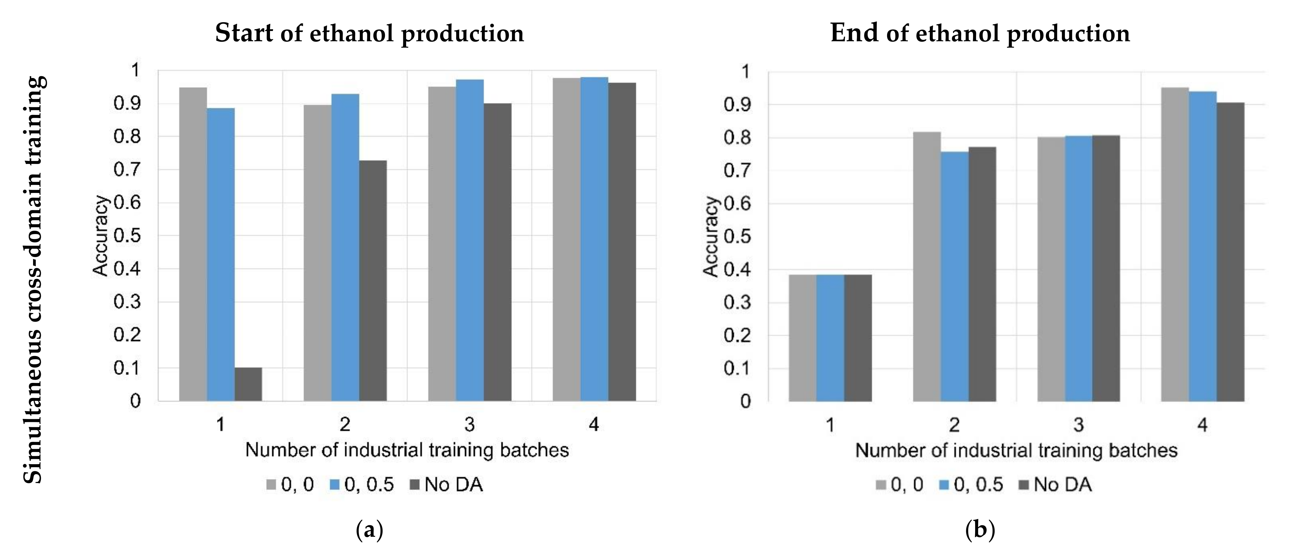
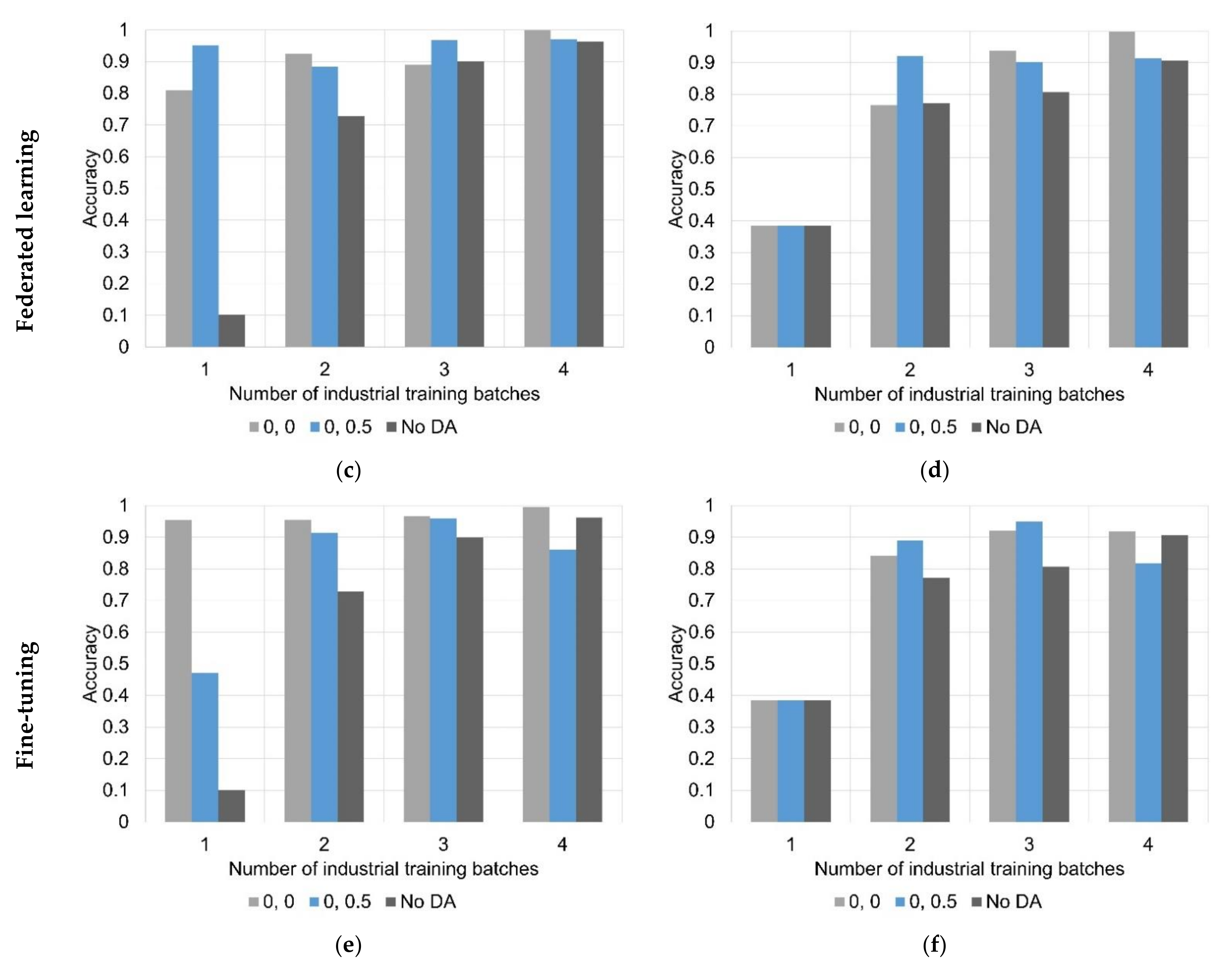
3.2. Machine Learning

Figure 5a,c,e and Figure 5b,d,f display the classification accuracies for the beginning of ethanol production and end of ethanol production for the trained networks, respectively. Although the multi-task networks were also trained to predict the time remaining until (and had passed since) the start and end of ethanol production, the regression predictions are most useful close to the classification boundaries. For example, an accurate prediction of the time since ethanol production started is not needed near the end of the fermentation process, or an approximate time for when ethanol production will end would not be useful when the fermentation is lagging and never begins. Therefore, the classification results are most valuable when evaluating the utility of the trained model. Furthermore, due to the multi-task nature of the model, the accuracy of the classification results correlates with the ability to learn the regression tasks close to the classification boundaries. As such, only the classification results are included in the presented graphs. However, the regression accuracies are presented in

Table 3. The regression accuracies of each of the models for predicting the time remaining until the start and end of ethanol production, where MAE is the Mean Absolute Error of the prediction. The base-line model was trained using only data from the industrial fermentations. The numbers in the Model column indicate the dropout probability used in each dropout layer. E.g., 0,0 represents 0 dropout probability in both layers.

Method	Model	Start of Ethanol Production Accuracy (MAE)				End of Ethanol Production Accuracy (MAE)
		1	2	3	4	1	2	3	4
Base-line model	No DA	2.769	1.099	0.646	0.710	2.035	1.278	1.047	0.534
Conventional domain adaptation	0, 0	1.942	0.93	0.423	0.541	1.767	0.980	0.950	0.681
	0, 0.5	3.326	1.528	0.836	0.171	7.29	2.027	1.528	0.920
Federated Learning	0, 0	2.496	0.540	0.431	0.726	3.884	1.133	0.599	0.351
	0, 0.5	2.482	0.423	0.520	0.296	3.073	1.089	0.937	0.663
Fine-tuning	0, 0	2.536	0.485	0.334	0.402	4.998	0.833	0.517	1.061
	0, 0.5	3.376	0.514	0.338	0.416	5.110	0.837	0.64	1.451

and discussed in the text.

Figure 5a,b display the results for the networks which were trained on the source and target domain data simultaneously. Preliminary investigations determined that the 0.5, 0.5 dropout rate models failed to train accurately for all training set sizes. Models with 0.5, 0 dropout rates produced inconsistent results, with some models accurately predicting using the test set data and some models performing worse than the model trained on only the industrial scale fermentations (No DA). However, the 0, 0 and 0, 0.5 models achieved higher accuracy than the No DA model for six out of eight classification tasks. Furthermore, the 0, 0 model achieved lower MAE for seven out of eight regression tasks compared to the No DA model. Therefore, the 0, 0 and 0, 0.5 dropout rates were used for subsequent investigations and the results of these models are presented in Figure 5a–f and Table 3. These higher accuracy results for the domain adaptation models prove that using the laboratory scale data to train the networks benefits the predictions on the industrial scale dataset.

Figure 5c,d display results for the models trained in a federated learning strategy. The two federated models are trained using the best performing dropout probabilities determined from the previous investigation and are compared with the No DA baseline results. The 0, 0 model achieved higher classification accuracies and lower MAE for six out of eight classification and regression tasks than the No DA model. When using four industrial scale fermentation batches in the training set, the 0, 0 model reached accuracies of 99.8% and 99.9% for predicting the start and end of ethanol production, respectively. Furthermore, the 0, 0.5 models achieved better results for seven out of eight of the classification and regression tasks. Overall, the federated learning models were more accurate than their corresponding non-federated training models using the same dropout probabilities, achieving higher classification accuracies on eight tasks compared to seven for the non-federated learning models. Similarly, the federated learning models achieved lower MAEs on 10 regression tasks compared with five for the non-federated learning models. This is an encouraging result as it indicates that not only can federated training provide benefits over models that train without the laboratory scale data, but that they can also perform better than conventionally trained domain adaptation networks in addition to maintaining data privacy. The reason for this may be the increased model learning afforded in the industrial scale dataset local model. During training, this model learns from an epoch full of the industrial scale training dataset compared with the non-federated model which only learns from the industrial scale target domain intermittently between source domain fermentation runs. This increased learning without switching between domains may allow the network weights to travel further towards local optima for the industrial scale dataset in each epoch. This contrasts with results presented in the wider literature, where federated learning degraded model accuracy compared with non-federated learning by 3.3% [50], 1.66% [51], and <10% [52].

Figure 5e,f display the classification results for the previously discussed federated models fine-tuned on the industrial dataset. While still providing improvements over the No DA base case, achieving higher classification accuracies for 12 out of 16 tasks, their accuracy is reduced over the starting federated learning models. This is most likely due to the fine-tuning method overfitting during training. The reason for this is the large network size required to learn both domains in the starting models. For example, the No DA models had a maximum optimum number of eight neurons in the fully connected layer and four LSTM units to learn only the target domain. However, the federated learning models required a maximum of 128 neurons in the fully connected layer and eight LSTM units to fit to both dataset domains. Therefore, when fine-tuning on the industrial dataset after fitting to both domains, the model begins to overfit, especially when four industrial batches are used in the training set.

3.3. Future Research Directions

Overall, transferring knowledge from the source domain increased model accuracy when applied to the target domain data. Using more than two datasets could increase this benefit further, especially using more similar datasets, e.g., from multiple industrial fermentation processes. The two datasets used in this work had distinct differences. For example, no temperature control on the laboratory scale dataset and an increasing time of flight during fermentation for the industrial scale dataset. It is anticipated that more similar datasets would provide even greater benefits. Furthermore, other than increasing model accuracy, the domain adaptation methodology can also reduce the time for ML model development. After training across two domains, the final models could be used to predict using data from a new fermentation process without having been trained on this new domain. However, incorporation of a small number of batches from this new fermentation process would be expected to aid model accuracy.

In this work, the waveform energy was the single feature used to describe the oscillating part of the US waveform. The reason for this was that previous work demonstrated that multiple oscillating waveform features are unlikely to follow similar trends across domains and their inclusion would degrade model accuracy [21]. However, for many applications of ML and US sensors, multiple features may need to be used to accurately monitor changes in this portion of the US waveform. In this case, the methodologies presented in this work may be used to obtain predictions on the target domain data from models trained on both the source and target domains. These predictions can then be used as an additional feature in a model only trained on the target domain data. In this way, other features describing the oscillating part of the waveform can be used as no domain adaptation is required while also incorporating knowledge from the source domain.

The combination of ML and US measurements should be used in further research over calibration procedures. In this work, the speed of sound increased during fermentation, agreeing with [14,15], which were conducted at large scale, but contradicting [16,17,49], which were conducted at small scale. This indicates that there is a discrepancy in the speed of sound trend at the ethanol, sugar, yeast, and CO₂ concentrations and temperature used at small and large scales. Therefore, extensive and complicated calibration procedures would need to be used to account for these effects. In addition, ML offers several distinct advantages: it negates the need for these complex calibration procedures accounting for all the parameters previously listed; more information from the waveforms is typically used through feature extraction; more complex fitting procedures are used, allowing for increased prediction accuracy; and validation procedures encourage model accuracy even on process parameters outside the range the model was trained on.

Acceptable ML model accuracy is dependent on its desired application. In this work, the highest accuracy model (federated learning, zero dropout, four industrial training batches) achieved 99.8% and 99.9% for predicting the start and end of ethanol production, respectively. This is equivalent to the current method of determination, off-line wort density measurements using hydrometers, which are only conducted once every several hours (or even less frequently overnight) and have reduced accuracy when foam is present. However, these model accuracies were obtained using only a single test set batch and therefore a large dataset size would be needed to determine whether these accuracies were consistent.

US measurements and ML could also be used in combination with sampling methods to reduce the amount of sampling required (and therefore also reducing operator burden), provide timely results between samples (for example, overnight), and predict when fermentation stages will be reached to improve plant scheduling. In this case, ML models can be continuously updated using the labelled data from the sample measurements. If US sensors are desired to eliminate the use of sampling, higher accuracy models would be required and longer model development times would be needed. In addition, a model that stated a confidence level of its prediction would increase trust in the model by identifying when sample measurements should be used as a safeguard.

4. Conclusions

This work has used previously collected US sensor data from laboratory scale fermentations to improve ML model accuracy on an industrial scale process. Overall, all methodologies led to improvements in model accuracy over training on the target domain alone. The federated learning methodology performed best, achieving higher accuracy for 14 out of 16 machine learning tasks compared with the base case model, and achieving around 100% test set accuracy when trained on four industrial datasets and no dropout was used. Federated learning improved model accuracy over the traditional simultaneous domain training by allowing increased tuning of the network weights to converge on local target domain optima. However, fine-tuning led to a decrease in model accuracy due to overfitting of networks caused by the larger number of neurons and LSTM units needed to accurately train on both domains. The methodologies investigated not only provide increased accuracy, but also speed up model development time by reducing the number of fermentation runs required to be monitored in the target domain.

References

1. Grassi, S.; Amigo, J.M.; Lyndgaard, C.B.; Foschino, R.; Casiraghi, E. Beer fermentation: Monitoring of process parameters by FT-NIR and multivariate data analysis. Food Chem. 2014, 155, 279–286. [Google Scholar] [CrossRef]
2. Jan, M.V.S.; Guarini, M.; Guesalaga, A.; Pérez-Correa, J.R.; Vargas, Y.; Perez-Correa, J. Ultrasound based measurements of sugar and ethanol concentrations in hydroalcoholic solutions. Food Control 2008, 19, 31–35. [Google Scholar] [CrossRef]
3. Vann, L.; Layfield, J.B.; Sheppard, J.D. The application of near-infrared spectroscopy in beer fermentation for online monitoring of critical process parameters and their integration into a novel feedforward control strategy. J. Inst. Brew. 2017, 123, 347–360. [Google Scholar] [CrossRef] [Green Version]
4. De Beer, T.; Burggraeve, A.; Fonteyne, M.; Saerens, L.; Remon, J.; Vervaet, C. Near infrared and Raman spectroscopy for the in-process monitoring of pharmaceutical production processes. Int. J. Pharm. 2011, 417, 32–47. [Google Scholar] [CrossRef] [PubMed] [Green Version]
5. Zhong, R.Y.; Xu, X.; Klotz, E.; Newman, S.T. Intelligent Manufacturing in the Context of Industry 4.0: A Review. Engineering 2017, 3, 616–630. [Google Scholar] [CrossRef]
6. Ghobakhloo, M. Industry 4.0, digitization, and opportunities for sustainability. J. Clean. Prod. 2020, 252, 119869. [Google Scholar] [CrossRef]
7. Corro-Herrera, V.A.; Gómez-Rodríguez, J.; Hayward-Jones, P.M.; Barradas-Dermitz, D.M.; Gschaedler-Mathis, A.C.; AguilarUscanga, M.G. Real-time monitoring of ethanol production during Pichia stipitis NRRL Y-7124 alcoholic fermentation using transflection near infrared spectroscopy. Eng. Life Sci. 2018, 18, 643–653. [Google Scholar] [CrossRef] [Green Version]
8. Wang, Q.; Li, Z.; Ma, Z.; Liang, L. Real time monitoring of multiple components in wine fermentation using an on-line auto-calibration Raman spectroscopy. Sens. Actuators B Chem. 2014, 202, 426–432. [Google Scholar] [CrossRef]
9. Schalk, R.; Frank, R.; Rädle, M.; Methner, F.-J.; Beuermann, T.; Braun, F.; Gretz, N. Non-contact Raman spectroscopy for in-line monitoring of glucose and ethanol during yeast fermentations. Bioprocess Biosyst. Eng. 2017, 40, 1519–1527. [Google Scholar] [CrossRef]
10. Mazarevica, G.; Diewok, J.; Baena, J.R.; Rosenberg, E.; Lendl, B. On-Line Fermentation Monitoring by Mid-Infrared Spectroscopy. Appl. Spectrosc. 2004, 58, 804–810. [Google Scholar] [CrossRef]
11. Veale, E.; Irudayaraj, J.; Demirci, A. An On-Line Approach to Monitor Ethanol Fermentation Using FTIR Spectroscopy. Biotechnol. Prog. 2007, 23, 494–500. [Google Scholar] [CrossRef]
12. Toledo, J.; Ruiz-Díez, V.; Pfusterschmied, G.; Schmid, U.; Sánchez-Rojas, J. Flow-through sensor based on piezoelectric MEMS resonator for the in-line monitoring of wine fermentation. Sens. Actuators B Chem. 2018, 254, 291–298. [Google Scholar] [CrossRef]
13. Ete-Carmona, E.C.; Gallego-Martinez, J.-J.; Martin, C.; Brox, M.; Luna-Rodriguez, J.-J.; Moreno, J. A Low-Cost IoT Device to Monitor in Real-Time Wine Alcoholic Fermentation Evolution through CO2 Emissions. IEEE Sens. J. 2020, 20, 6692–6700. [Google Scholar] [CrossRef]
14. Hussein, W.B.; Hussein, M.A.; Becker, T. Robust spectral estimation for speed of sound with phase shift correction applied online in yeast fermentation processes. Eng. Life Sci. 2012, 12, 603–614. [Google Scholar] [CrossRef]
15. Hoche, S.; Krause, D.; Hussein, M.A.; Becker, T. Ultrasound-based, in-line monitoring of anaerobe yeast fermentation: Model, sensor design and process application. Int. J. Food Sci. Technol. 2016, 51, 710–719. [Google Scholar] [CrossRef]
16. Resa, P.; Elvira, L.; De Espinosa, F.M. Concentration control in alcoholic fermentation processes from ultrasonic velocity measurements. Food Res. Int. 2004, 37, 587–594. [Google Scholar] [CrossRef]
17. Resa, P.; Elvira, L.; De Espinosa, F.M.; González, R.; Barcenilla, J. On-line ultrasonic velocity monitoring of alcoholic fermentation kinetics. Bioprocess Biosyst. Eng. 2008, 32, 321–331. [Google Scholar] [CrossRef]
18. Bowler, A.; Escrig, J.; Pound, M.; Watson, N. Predicting Alcohol Concentration during Beer Fermentation Using Ultrasonic Measurements and Machine Learning. Fermentation 2021, 7, 34. [Google Scholar] [CrossRef]
19. Donadini, G.; Porretta, S. Uncovering patterns of consumers’ interest for beer: A case study with craft beers. Food Res. Int. 2017, 91, 183–198. [Google Scholar] [CrossRef]
20. Gatrell, J.; Reid, N.; Steiger, T.L. Branding spaces: Place, region, sustainability and the American craft beer industry. Appl. Geogr. 2018, 90, 360–370. [Google Scholar] [CrossRef]
21. Bowler, A.L.; Watson, N.J. Transfer learning for process monitoring using reflection-mode ultrasonic sensing. Ultrasonics 2021, 115, 106468. [Google Scholar] [CrossRef] [PubMed]
22. Kouw, W.M.; Loog, M. A Review of Domain Adaptation without Target Labels. IEEE T Pattern Anal. 2021, 43, 766–785. [Google Scholar] [CrossRef] [PubMed] [Green Version]
23. Li, X.; Zhang, W.; Ding, Q.; Sun, J.-Q. Multi-Layer domain adaptation method for rolling bearing fault diagnosis. Signal Process. 2019, 157, 180–197. [Google Scholar] [CrossRef] [Green Version]
24. Li, X.; Zhang, W.; Ding, Q. A robust intelligent fault diagnosis method for rolling element bearings based on deep distance metric learning. Neurocomputing 2018, 310, 77–95. [Google Scholar] [CrossRef]
25. Guo, L.; Lei, Y.; Xing, S.; Yan, T.; Li, N. Deep Convolutional Transfer Learning Network: A New Method for Intelligent Fault Diagnosis of Machines with Unlabeled Data. IEEE T. Ind. Electron. 2019, 9, 7316–7325. [Google Scholar] [CrossRef]
26. Lu, W.; Liang, B.; Cheng, Y.; Meng, D.; Yang, J.; Zhang, T. Deep Model Based Domain Adaptation for Fault Diagnosis. IEEE T. Ind. Electron. 2017, 3, 2296–2305. [Google Scholar] [CrossRef]
27. Geng, B.; Tao, D.; Xu, C. DAML: Domain adaptation metric learning. IEEE T. Image Process. 2011, 10, 2980–2989. [Google Scholar] [CrossRef]
28. Tzeng, E.; Hoffman, J.; Saenko, K.; Darrell, T. Adversarial discriminative domain adaptation. Proc. CVPR IEEE 2017, 2017, 2962–2971. [Google Scholar] [CrossRef] [Green Version]
29. Zhang, W.; Ouyang, W.; Li, W.; Xu, D. Collaborative and Adversarial Network for Unsupervised Domain Adaptation. Proc. CVPR IEEE 2018, 2018, 3801–3809. [Google Scholar] [CrossRef]
30. Zhang, Y.; Qiu, Z.; Yao, T.; Liu, D.; Mei, T. Fully Convolutional Adaptation Networks for Semantic Segmentation. Proc. CVPR IEEE 2018, 2018, 6810–6818. [Google Scholar] [CrossRef] [Green Version]
31. Tsai, Y.-H.; Hung, W.-C.; Schulter, S.; Sohn, K.; Yang, M.-H.; Chandraker, M. Learning to Adapt Structured Output Space for Semantic Segmentation. Proc. CVPR IEEE. 2018, 2018, 7472–7481. [Google Scholar] [CrossRef] [Green Version]
32. Chen, W.; Wang, H.; Li, Y.; Su, H.; Wang, Z.; Tu, C.; Lischinski, D.; Cohen-Or, D.; Chen, B. Synthesizing training images for boosting human 3D pose estimation. Proc. 3DV 2016, 2016, 479–488. [Google Scholar] [CrossRef] [Green Version]
33. Sankaranarayanan, S.; Balaji, Y.; Castillo, C.D.; Chellappa, R. Generate to Adapt: Aligning Domains Using Generative Adversarial Networks. Proc. CVPR IEEE 2018, 2018, 8503–8512. [Google Scholar] [CrossRef] [Green Version]
34. Sankaranarayanan, S.; Balaji, Y.; Jain, A.; Lim, S.N.; Chellappa, R. Learning from Synthetic Data: Addressing Domain Shift for Semantic Segmentation. Proc. CVPR IEEE 2018, 2018, 3752–3761. [Google Scholar] [CrossRef] [Green Version]
35. Bousmalis, K.; Silberman, N.; Dohan, D.; Erhan, D.; Krishnan, D. Unsupervised pixel-level domain adaptation with generative adversarial networks. Proc. CVPR IEEE 2017, 2017, 95–104. [Google Scholar] [CrossRef] [Green Version]
36. Bousmalis, K.; Irpan, A.; Wohlhart, P.; Bai, Y.; Kelcey, M.; Kalakrishnan, M.; Downs, L.; Ibarz, J.; Pastor, P.; Konolige, K.; et al. Using Simulation and Domain Adaptation to Improve Efficiency of Deep Robotic Grasping. IEEE Int. Conf. Robot. 2018, 2018, 4243–4250. [Google Scholar] [CrossRef] [Green Version]
37. Zhang, W.; Peng, G.; Li, C.; Chen, Y.; Zhang, Z. A new deep learning model for fault diagnosis with good anti-noise and domain adaptation ability on raw vibration signals. Sensors 2017, 17, 425. [Google Scholar] [CrossRef]
38. Du, Y.; Jin, W.; Wei, W.; Hu, Y.; Geng, W. Surface EMG-based inter-session gesture recognition enhanced by deep domain adaptation. Sensors 2017, 17, 458. [Google Scholar] [CrossRef] [Green Version]
39. Han, Y.; Yoo, J.; Kim, H.H.; Sin, H.J.; Sung, K.; Ye, J.C. Deep learning with domain adaptation for accelerated projection-reconstruction MR. Magn. Reson. Med. 2018, 80, 1189–1205. [Google Scholar] [CrossRef] [Green Version]
40. Yang, Q.; Liu, Y.; Chen, T.; Tong, Y. Federated machine learning: Concept and applications. ACM T. Intel. Syst. Tec. 2019, 10, 12. [Google Scholar] [CrossRef]
41. Kirkpatrick, J.; Pascanu, R.; Rabinowitz, N.; Veness, J.; Desjardins, G.; Rusu, A.A.; Milan, K.; Quan, J.; Ramalho, T.; Grabska-Barwinska, A.; et al. Overcoming catastrophic forgetting in neural networks. Proc. Natl. Acad. Sci. USA 2017, 114, 3521–3526. [Google Scholar] [CrossRef] [Green Version]
42. McClements, D. Advances in the application of ultrasound in food analysis and processing. Trends Food Sci. Technol. 1995, 6, 293–299. [Google Scholar] [CrossRef]
43. Zhan, X.; Jiang, S.; Yang, Y.; Liang, J.; Shi, T.; Li, X. Inline Measurement of Particle Concentrations in Multicomponent Suspensions using Ultrasonic Sensor and Least Squares Support Vector Machines. Sensors 2015, 15, 24109–24124. [Google Scholar] [CrossRef] [Green Version]
44. Henning, B.; Rautenberg, J. Process monitoring using ultrasonic sensor systems. Ultrasonics 2006, 44, e1395–e1399. [Google Scholar] [CrossRef]
45. Li, X.; Zhao, L.; Wei, L.; Yang, M.-H.; Wu, F.; Zhuang, Y.; Ling, H.; Wang, J. DeepSaliency: Multi-Task Deep Neural Network Model for Salient Object Detection. IEEE T. Image Process. 2016, 25, 3919–3930. [Google Scholar] [CrossRef] [Green Version]
46. Hochreiter, S.; Schmidhuber, J. Long Short-Term Memory. Neural Comput. 1997, 9, 1735–1780. [Google Scholar] [CrossRef]
47. Machine Learning Mastery. Available online: https://machinelearningmastery.com/handle-long-sequences-long-short-termmemory-recurrent-neural-networks/ (accessed on 11 August 2021).
48. Srivastava, N.; Hinton, G.; Krizhevsky, A.; Sutskever, I.; Salakhutdinov, R. Dropout: A simple way to prevent neural networks from overfitting. J. Mach. Learn. Res. 2014, 15, 1929–1958. [Google Scholar]
49. Lamberti, N.; Ardia, L.; Albanese, D.; Di Matteo, M. An ultrasound technique for monitoring the alcoholic wine fermentation. Ultrasonics 2009, 49, 94–97. [Google Scholar] [CrossRef]
50. Chen, Y.-T.; Chunag, Y.-C.; Wu, A.-Y.A. Online Extreme Learning Machine Design for the Application of Federated Learning. In Proceedings of the IEEE International Conference on Artificial Intelligence Circuits and Systems (AICAS), Genova, Italy, 31 August–2 September 2020; pp. 188–192. [Google Scholar] [CrossRef]
51. Dib, M.A.D.S.; Ribeiro, B.; Prates, P. Federated Learning as a Privacy-Providing Machine Learning for Defect Predictions in Smart Manufacturing. Smart Sustain. Manuf. Syst. 2021, 5, 1–17. [Google Scholar] [CrossRef]
52. Ge, N.; Li, G.; Zhang, L.; Liu, Y. Failure prediction in production line based on federated learning: An empirical study. J Intell Manuf. 2021. [Google Scholar] [CrossRef]
Figure 1. The probe consisting of US and temperature sensors and the paths of the received US sound wave reflections. Adapted from [18].
Fermentation 07 00253 g001
Figure 2. An example US waveform acquired: (a) The full waveform received; (b) the 1st reflection isolated; (c) the 2nd reflection isolated; and (d) the 3rd reflection isolated.
Fermentation 07 00253 g002aFermentation 07 00253 g002b
Figure 3. US feature and temperature results for the five industrial fermentation batches. (a) The process temperature. (b) The process temperature until one day post the end of ethanol production. (c) The first reflection energy until one day post the end of ethanol production. (d) The third reflection energy until one day post the end of ethanol production. (e) The first reflection time of flight measured using a thresholding method until one day post the end of ethanol production. (f) The third reflection time of flight measured using a thresholding method until one day post the end of ethanol production.
Fermentation 07 00253 g003
Figure 4. The first reflection energy for the first five laboratory scale fermentation batches.
Fermentation 07 00253 g004
Figure 5. The classification results on the industrial scale fermentations test set. The numbers in the legend indicate the dropout layer probability for the two dropout layers. E.g., 0, 0 indicates a dropout probability of zero in both layers. (a) Classification results for the start of ethanol production for the networks trained on both domain datasets simultaneously. (b) Classification results for the end of ethanol production for the networks trained on both domain datasets simultaneously. (c) Classification results for the start of ethanol production for the networks trained using federated learning. (d) Classification results for the end of ethanol production for the networks trained using federated learning. (e) Classification results for the start of ethanol production for the federated training networks fine-tuned on the industrial scale dataset. (f) Classification results for the end of ethanol production for the federated training networks fine-tuned on the industrial scale dataset.
Fermentation 07 00253 g005aFermentation 07 00253 g005b