1. Introduction
Winemaking has been a part of civilisation since as early as 6000 BC, with signs of winemaking practices being documented in Mesopotamia and Caucasus [
1]. In modern times, winemaking is a worldwide industry, with many countries being frontrunners [
2]. As such, this leads to a highly competitive global market, where consistency and quality are required by the wine buyers [
3].
With new technologies becoming available and rapid improvement in software and computing, more methods to monitor parameters of oenological importance have become available and more widely used. In particular, the use of spectroscopic technologies is becoming commonplace, with infrared and fluorescence being applied to many industries [
4]. Due to their availability, robustness, and non-destructive nature, near-infrared (NIR) and mid-infrared (MIR) spectroscopy in conjunction with chemometrics has become an area of interest in both industrial and research communities for this purpose [
5,
6,
7,
8,
9,
10]. As with most industrial processes, the control of the winemaking process is essential to avoiding problems that may arise leading to low-quality wines and, therefore, the loss of a competitive edge [
11]. Previously, time-consuming and, often, destructive methods were used to quantify certain phenolic and oenological parameters during fermentation [
7].
Phenolic components present in wine contribute to the sensory qualities such as mouthfeel, colour, and taste [
12,
13]. As such, measuring and monitoring the extraction of these compounds during fermentation is an important aspect to ensuring that quality parameters are achieved and process control is maintained [
9,
14]. Robust and multivariate models utilising both NIR and MIR instrumentation have been developed to quantify oenological parameters; however, these rely on discrete samples that have received treatments to remove particles in suspension [
11,
15,
16]. To our knowledge, there have been no attempts to build or optimise PLS calibrations for phenolic parameters or the concentration of phenolic compounds in minimally treated (filtered) or untreated red-wine samples using infrared spectroscopy.
In a previous study, the effect of different sample treatments on spectral data was evaluated [
17]. Promising PLS calibrations were built for the quantification of phenolic parameters during wine fermentation using samples that received different sample treatments, in the form of freezing, centrifugation and filtration. The purpose of this study is to further move towards automated and in-line methods of analysis by optimising calibrations with spectral data from samples receiving minimal (rough filtration) or no treatment, as these would more accurately represent measurements taken directly from a fermentation vessel. The robustness and accuracy of the models and whether the models are applicable during the entire duration of the fermentation, especially from the very beginning when lower phenolic levels are present, was evaluated. The limit of detection and quantification was therefore assessed and considered during the optimisation process. The suitability of three different infrared spectroscopic techniques for in-line implementation, namely attenuated-transmission Fourier-transform mid-infrared (ATR-FT-MIR), transmission Fourier-transform near-infrared (T-FT-NIR) and diffuse-reflectance Fourier-transform near-infrared (DR-FT-NIR), was investigated. ATR-FT-MIR was selected as one method as it has shown promise regarding turbid and opaque samples and would be suitable for an in-line application. For the NIR technologies, the diffuse-reflectance method was chosen due to its contactless nature, allowing for the non-invasive analysis of samples. Finally, the T-FT-NIR technology was chosen as the availability of the liquid probe attachment could potentially lend itself to installation in piping and tanks in industrial applications [
17].
2. Materials and Methods
2.1. Small-Scale Vinifications and Sample Treatment
One hundred and twenty kilograms of Shiraz and Cabernet Franc grapes were collected from a collaborating cellar in the Stellenbosch region of South Africa. Before crushing and destemming took place, the grapes were stored at 4 °C for two days. To ensure homogeneity between the 20 kg fermentations, the juice and skins of each cultivar were mixed thoroughly in a bin after crushing and destemming before subdivision. Once subdivided, the SO2 concentration was adjusted to 30 ppm using a 2% SO2 solution. Each fermentation was moved into a fermentation room held at 25 °C. A strain of Saccharomyces cerevisiae Lalvin ICV D21® (Lallemand, Montreal, QC, Canada) was used for alcoholic fermentation. Inoculation was performed according to manufacturer’s instructions. This yeast was chosen due to its suitability for producing red wines with stable colour, as well as its high alcohol tolerance and good fermentative performance.
Half of the fermentations received enzymatic treatments at the same time as inoculation with S. cerevisiae. The enzyme used was Lafase® HE Grand CRU Vin Rouge (Laffort, Bordeaux, France), consisting of pectolytic enzymes, and rehydration and dosing was performed according to manufacturer’s instructions. During the AF, three punch downs were done at 08:00, 12:00 and 16:00 each day until alcoholic fermentation was completed. Samples were collected immediately after the 08:00 punch down and during 9 days of fermentation. Briefly, the sample was subdivided into equal volumes and each volume received different pre-treatments. The two pre-treatments of interest for this study were filtration through a 400 µm mesh (Xylem Floject Process Pump Filter, RS Components) and no pre-treatment (direct sample from the fermenting vessel). Two-millilitre samples were used for ATR-MIR spectroscopy whilst 20 mL samples were used for FT-NIR spectroscopy.
2.2. Spectral Data Acquisition
2.2.1. ATR-FT-MIR Spectroscopy
An Alpha-P Attenuated Total Reflectance Fourier Transform Mid Infrared (ATR-FT-MIR) spectrometer (Bruker Optics, Ettligen, Germany) with a 2 mm
2 single bounce diamond sample plate was used to obtain the spectra in a closed environment. A resolution of 4 cm
−1 was used over a range of 4000–400 cm
−1 and 128 sample scans at a temperature of 30 °C were acquired. The resolution was chosen as it provided well-defined spectra whilst also allowing for time-efficient scanning. Prior to sample scanning, a background spectrum was obtained using distilled water and was repeated every 2 h. All control and selections were performed using OPUS Wine Wizard (OPUS v7.0 for Microsoft, Bruker Optics, Ettlingen, Germany). The average ATR-FT-MIR spectra for filtered and untreated samples are reported in
Figure 1.
2.2.2. Transmission FT-NIR Spectroscopy
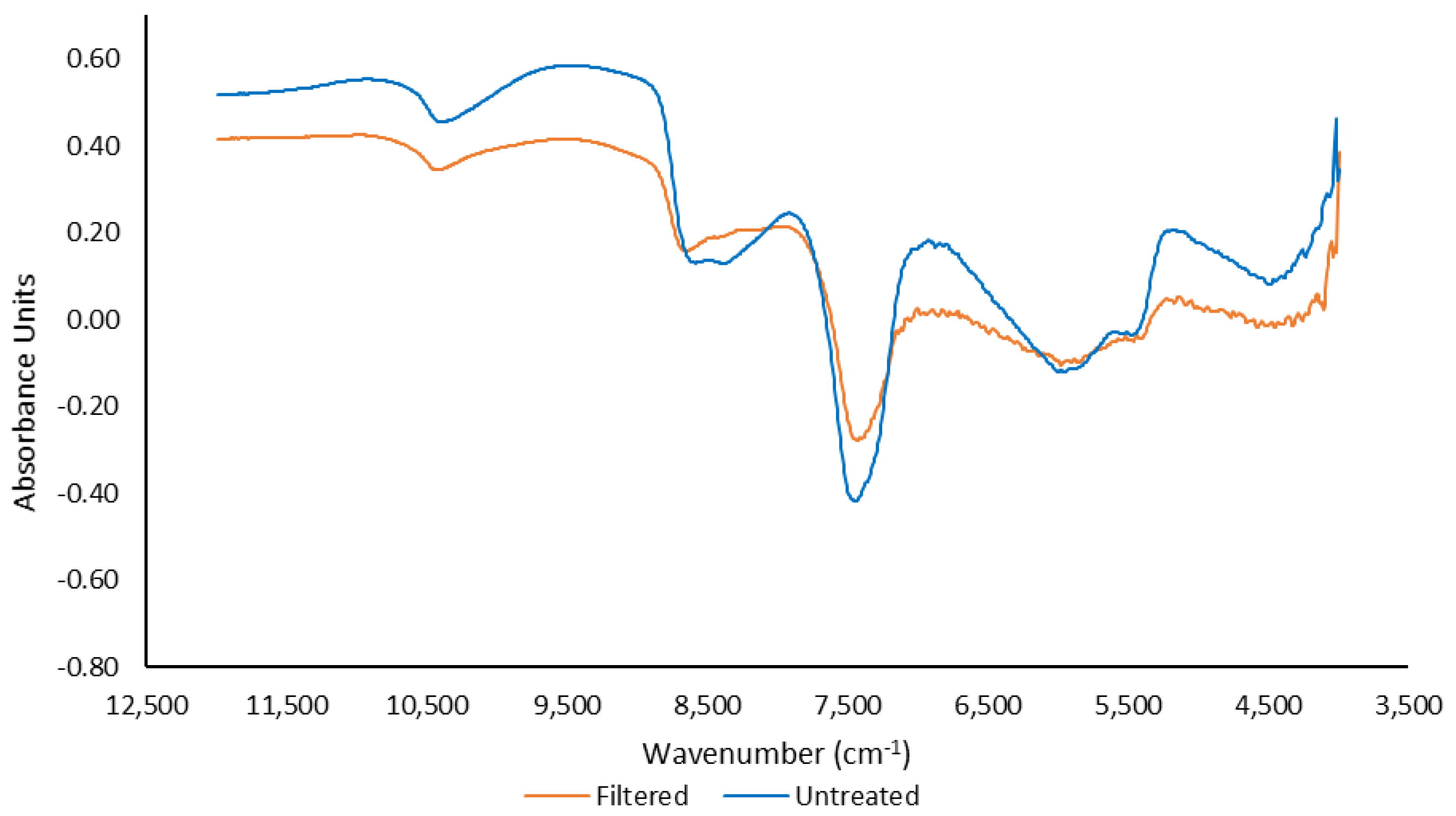
Transmission Fourier-transform near-infrared (T-FT-NIR) was performed using the liquid probe attachment of the Multi-purpose analyser (MPA) FT-NIR instrument (Bruker Optics, Ettlingen, Germany). A resolution of 2 cm
−1 was used over a range of 12,500–4000 cm
−1 for 64 sample scans at ambient temperature. An air background spectrum was taken prior to scanning and then every two hours. All control and selections were made using OPUS for Microsoft, Bruker Optics, Ettlingen, Germany). The average T-FT-NIR spectra for filtered and untreated samples are reported in
Figure 2.
2.2.3. Diffuse-Reflectance FT-NIR Spectroscopy
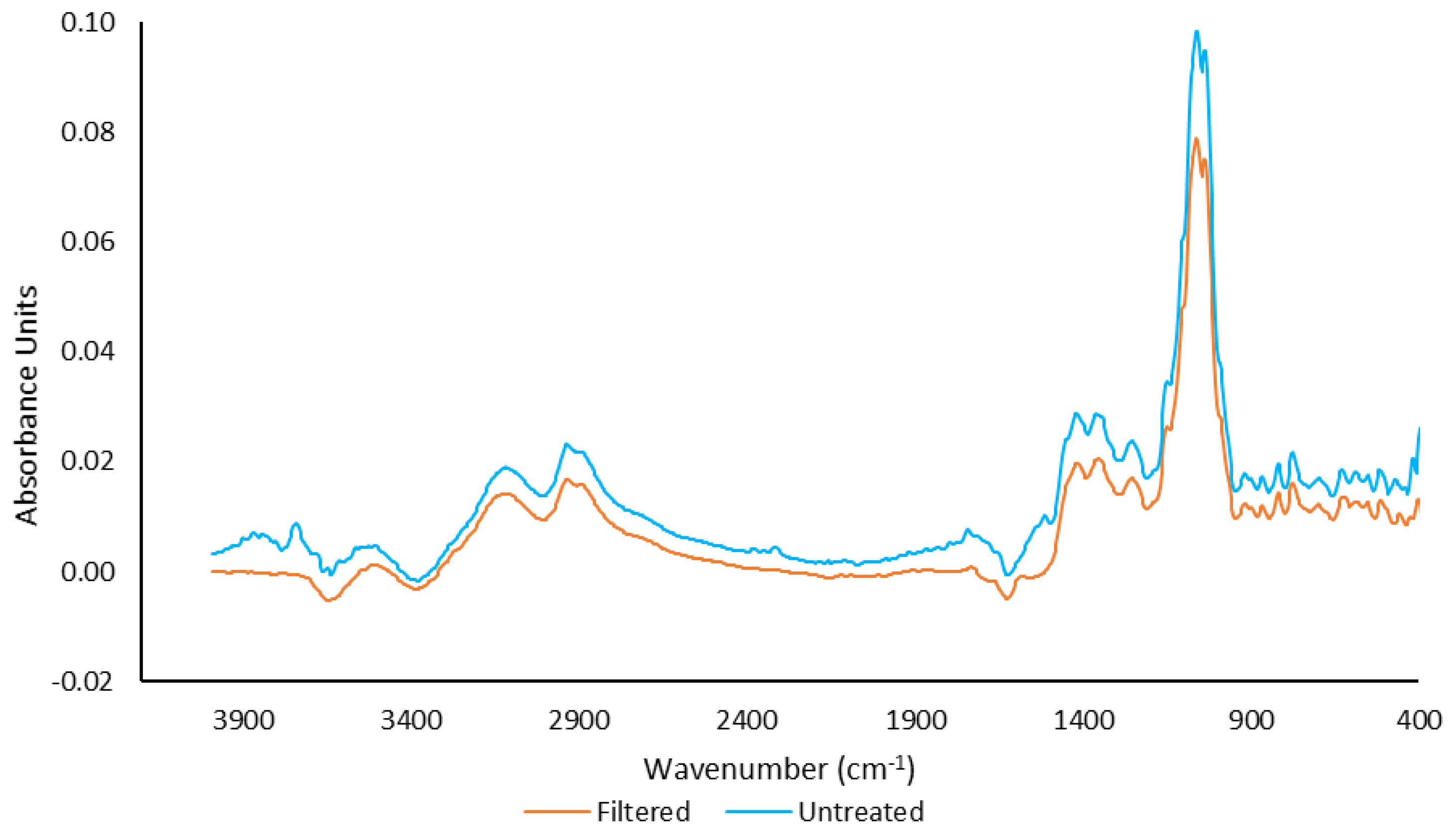
Spectra were also collected using a contactless Matrix DR-FT-NIR spectrometer in diffuse-reflectance mode (DR-FT-NIR) (Bruker Optics, Ettlingen, Germany). For sample scanning, two of the four existing tungsten bulbs (12 V, 20 W) were used with a 17 cm measuring distance. A background spectrum was obtained prior to scanning using a 20 mL volume of distilled water in a clear glass container. Sixty-four sample scans were performed over a wavenumber range of 12,500–4000 cm
−1 at a resolution of 16 cm
−1. The average DR-FT-NIR spectra for filtered and untreated samples are reported in
Figure 3.
2.3. Iland Analysis for Total Anthocyanin and Total Phenolic Content
For the quantification of total anthocyanin content as well as the total phenolic index of the samples, the method reported by Iland et al. (2000) was used [
15,
18]. Briefly, this involves the dilution of a 100 µL sample of fermenting must in 5 mL of 1 M HCl after centrifugation of the sample. This is then left in the dark for one hour [
19]. A Multiskan GO Microplate Spectrophotometer (Thermo Fisher Scientific, Inc., Waltham, MA, USA) was used to measure the absorbances of 200 µL of the samples at 520 nm and 280 nm for each component, respectively. To obtain the total phenolics index (TPI), the absorbance measured at 280 nm was multiplied by the dilution factor. The anthocyanin content was quantified in terms of malvidin-3-glucoside equivalents, with the use of the following equation [
15]:
where A520 nm refers to the measured absorbance at 520 nm, MW and ε refer to the molecular weight of malvidin-3-glucoside (529 g/mol) and the extinction coefficient (28,000 L/(cm mol)) of this compound, respectively, DF represents the dilution factor and L refers to the 1 cm pathlength used.
2.4. Methylcellulose-Tannin-Precipitation Assay
The concentration of tannins in the samples was quantified using a high-throughput method adapted by Mercurio, Dambergs, Herderich, and Smith (2007). The reagents required for this include a 0.04%
w/v methylcellulose solution as well as a saturated ammonium-sulphate solution [
20]. The method requires both a control receiving no methylcellulose and a treated sample receiving the solution. To prepare the control, a 50 µL measure of a sample was added to a 2 mL microfuge tube, followed by 400 µL of the saturated ammonium-sulphate solution and, finally, topped up with 1550 µL of distilled water. Preparation of the sample receiving treatment involved adding 600 µL of the methylcellulose solution to a 50 µL measure of the sample. After an elapsed time of three minutes, 400 µL of saturated ammonium sulphate was added and 950 µL of distilled water was used to bring the volume to 2 mL. Both control and treatment were centrifuged at 11,180 ×
g for 5 min using an Eppendorf 5415 D (Hamburg, Germany) centrifuge after allowing precipitation of the tannins to occur (10 min). The absorbances at 280 nm was measured for both the control and treatment. The difference between these values was used to determine the concentration of tannins with the use of a calibration curve using epicatechin equivalents and multiplication by the dilution factor. This calibration curve was generated by making a 1 g/L epicatechin (E1753, Merck, Darmstadt, Germany) stock solution using 0.1 g of epicatechin and 100 mL of 96.4% ethanol. This stock solution was further used to make a dilution series with concentrations in the range 0.025 g/L–0.3 g/L. Two-hundred microliters of each solution in the dilution series was scanned at 280 nm using distilled water as a blank.
2.5. Colour Density
Fifty µL of each sample was pipetted into a 96-well microplate (Thermo Fisher Scientific, Inc., Waltham, MA, USA) and the total absorbance measured at 420 nm, 520 nm and 620 nm with distilled water as a blank. The sum of these absorbances yielded the colour density [
21].
2.6. SO2-Resistant Pigments
To quantify the concentration of SO
2-resistant pigments in a sample, the modified Somers Assay, adapted by Mercurio, Dambergs, Herderich, and Smith (2007), was used. A buffer solution consisting of model wine (0.5%
w/v tartaric acid and 12%
v/v ethanol adjusted to a pH of 3.4 using 1 M NaOH solution) was used. A 200 µL measure of a sample was diluted with 1.8 mL of the buffer solution with 0.375%
w/v sodium metabisulphite [
20]. After addition of reagents and vortexing, the samples stood for an hour at room temperature. Finally, the absorbance of 200 µL at 520 nm was measured. Using the previous equation for anthocyanin quantification, the final levels of SO
2-resistant pigments were obtained.
2.7. Development and Validation of PLS Calibrations
All modelling and evaluation of the models were performed using PLS Toolbox 8.8 for MATLAB R2019b (Mathworks Inc., Natik, MA, USA). The data set was split into a calibration and test set with a ratio of 66/34, respectively. For the calibration, the optimal number of latent variables was calculated using a cross-validation procedure. For this, the venetian-blinds approach was used with 10 data splits. To determine the best pre-processing method and wavenumber selection for a particular variable, pre-processing algorithms (including no pre-processing) were considered using both forward and backward iPLS interval selection. The pre-processing options and interval selection that corresponded with the lowest root mean square error (RMSECV) were selected for further model optimisation.
Certain statistics were used to determine the accuracy and reliability of the models. The coefficient of correlation for calibration (R
2cal) and validation (R
2val) was used to explain the percentage of variation. Although this is not the only requirement for a model to be considered accurate, it is necessary for the respective R
2 value to be as close to 1 as possible. On the contrary, low values are indicative of either poor correlation between spectra and the reference values or poor reproducibility in the reference methods themselves [
15]. Another value used was the root mean square error (RMSE), which is a measure of the difference between predicted values and the true values determined by the reference methods [
22]. This value, therefore, provides the average prediction error and is reported in the same units as the reference values. Values are reported for both calibration (RMSECV) and prediction (RMSEP) [
23]. Residual predictive deviation (RPD) is the ratio of standard deviation of the data set to the RMSE and is calculated as the standard deviation of the population divided by the root mean standard error for both calibration (RPDcal) and validation (RPDval) [
24]. The higher the RPD, the higher the ability of the model to accurately predict new samples.
Further, slope and intercept tests, as reported by Linnet [
25], were used in each case to determine if systematic error existed between the predicted values and reference values or if the differences were a product of random noise. This method of analysis makes no assumptions regarding which set of values is the reference. The null hypothesis is accepted if the slope is found to be 1 and the y-intercept is found to be 0 at 95% confidence intervals. This test is used to compare the predicted values and the reference values for a particular model and the predicted values for sample treatments as well as different instruments. The inter-class correlation (ICC) is a value that is used to determine the consistency values predicted by the models and was used in the validations of the models and in the comparisons between sample treatments and instruments [
26]. ICC can range from 0 to 1, where a value of 1 indicates perfect reliability, and, therefore, values as close to 1 as possible are desirable. Finally, the standard error of measurement (SEM) was also used to validate the models. This method can determine the precision of each individual measurement, and can, therefore, provide an absolute value of the reliability of a model [
22].
The limit of detection (LOD) and limit of quantification (LOQ) of the PLS calibrations were also calculated and used to determine at which point in the fermentation the model could be accurately applied. The regression coefficients of the calculated PLS regression model are used in conjunction with the standard deviations (uncertainties) of the reference and spectroscopic methods to calculate the LOD and LOQ. This is possible as the LOD is an indication of the lowest concentration of an analyte that can be detected and therefore accurately predicted. The LOQ is calculated at three times the LOD [
27].
4. Discussion
NIR and MIR spectroscopy is already beneficial in that it is rapid, non-destructive and requires very little sample preparation [
11,
35,
36]. The incorporation of samples that are more representative of those taken directly from a tank is another step in moving towards better process control in the wine industry. Developed PLS regression models often make use of spectral pre-processing techniques to improve the accuracy and reliability of the models [
7,
9,
14,
37]. In addition, wavenumber selection is common when developing calibrations once fingerprint regions have been identified. Further, the applicability of a model is also dependent on the limit of detection, as this will determine at what point in the fermentation it can be applied. This metric has been reported in studies conducted on wine fermentations [
7,
15].
To our knowledge, this is the first study of its kind, seeking to use IR technology and chemometric techniques to optimise PLS regression models for phenolic compounds in minimally treated or untreated wine/must samples. A study by Shrake et al., 2014 demonstrated that non-destructive, in-line monitoring of colour and total phenolic content of red wine is a possibility, with very positive results. In this study, samples were filtered in line using a 2 µm filter and analysed using light-emitting-diode sensors. However, in this study, yeast and pulp were removed with the use of peristaltic pumps before scanning took place [
38]. The remaining particles, therefore, did not exceed 2 µm in size when scanning took place. In contrast, this study incorporates samples where the size of the solid particulates is not controlled by means of a filter (untreated) or in samples where the size of the particles would not exceed 400 µm in size. This study, therefore, allows for more simplistic in-line monitoring, as finer filters would not need to be incorporated into the system for sampling purposes. However, one aspect addressed in Shrake et al., 2014, which would be beneficial to this study is the development of an in-line flow cell, which would replace the physical instrument.
New PLS calibrations for three different spectroscopic methods, namely ATR-FT-MIR, DR-FT-NIR, and T-FT-NIR, were optimised. The models for ATR-FT-MIR were shown to be suitable for use in industry, as they showed sufficient accuracy while also having an LOD and LOQ suitable for lower levels of phenolic compounds. This was the case for ATR-FT-MIR for samples that were filtered and those that received no treatment. This is consistent with how this spectroscopic method functions. As the IR radiation is only allowed to penetrate the sample by 2 µm [
39], entrained gasses and solid particles are expected not to have a substantial influence when the spectra are obtained. In the case of ATR-FT-MIR, it appears that filtration is more desirable than completely untreated samples. Models with good performance metrics can be expected from instrumentation such as this in a setting where samples will be taken directly from a fermentation vessel. Of the three spectroscopic acquisition methods, the ATR-FT-MIR had the best performance, allowing for accuracy as well as versatility in monitoring a fermentation.
DF-FT-NIR spectroscopy relies on variations in direction and intensity in the IR radiation after it has reflected from a sample’s surface [
40]. When considering the PLS calibrations built, the most suitable models were those built with filtered samples, as these models showed good performance in all the metrics. For samples with higher levels of turbidity, the scattering may be too intense, causing lower performance. The spectral pre-processing allows for better LOD and LOQ whilst still ensuring that RPD values remain high enough for practicality and reliability. As with the ATR-FT-MIR, these models show promise with regards to industrial application.
In the case of T-FT-NIR, the performance was substantially lower than that of the other two techniques. The spectral pre-processing and wavenumber selection appeared to have little effect on model improvement when untreated samples were used, and the models built using these techniques showed higher LODs and LOQs in conjunction with lower RPD values. However, it should still be noted that in certain cases, namely for polymeric pigments and TPI, the models were still appropriate for industrial application. In these cases, it might be pertinent to include better filtration techniques to improve the accuracy and reliability of the other PLS calibrations relying on this method.
With the ease of using the instrument and a further reduction in necessary sample treatment, these calibrations can be applied to in-line sampling systems. When deploying models in an industrial setting, it would be beneficial to incorporate a more complete sample set during the modelling stage that consists of a range of different cultivars and fermenting samples with a wide enough range of values for each phenolic component. These models used in conjunction with process-control software can lead to the incorporation of alarms and warnings, thereby providing an easier way for winemakers to control their fermentations. As most of the models showed good performance and suitability, it would be beneficial to consider other aspects such as cost and ease of installation when selecting a final system to be deployed.


