
Lactic Acid Production from Cow Manure: Technoeconomic Evaluation and Sensitivity Analysis


Abstract
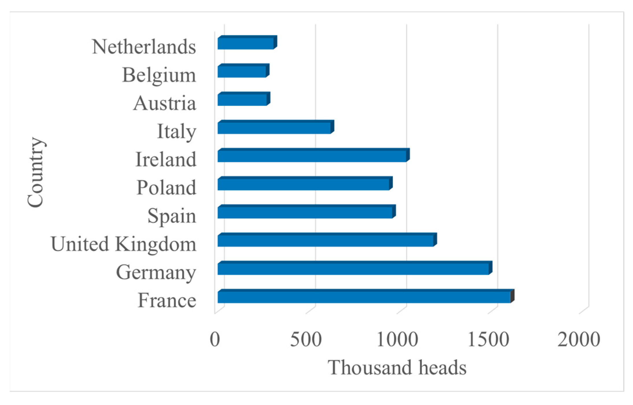
:1. Introduction
2. Materials and Methods
2.1. Raw Material and Strain
2.2. Process Model Simulation and Scenario Design
2.3. Process Design
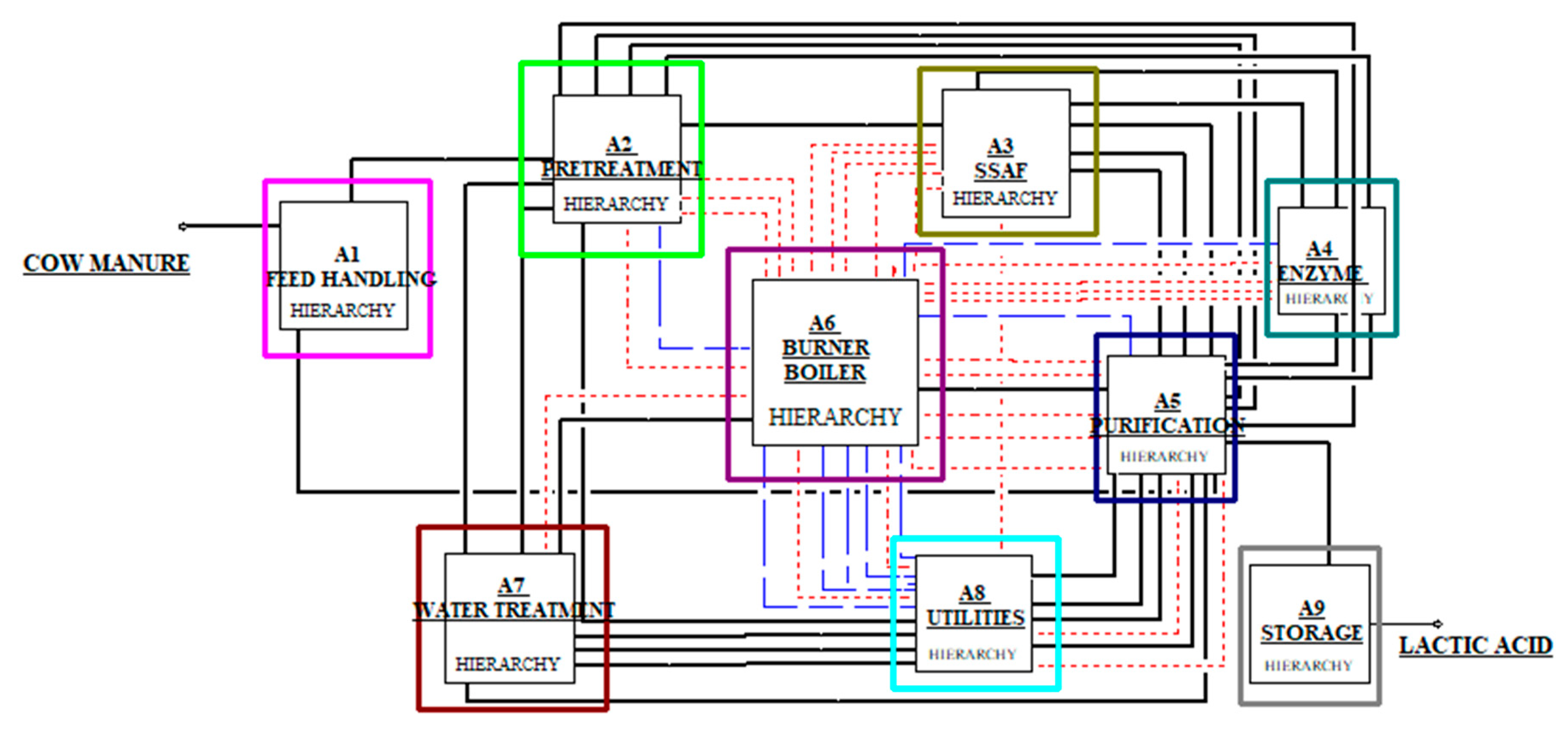
2.3.1. General Process
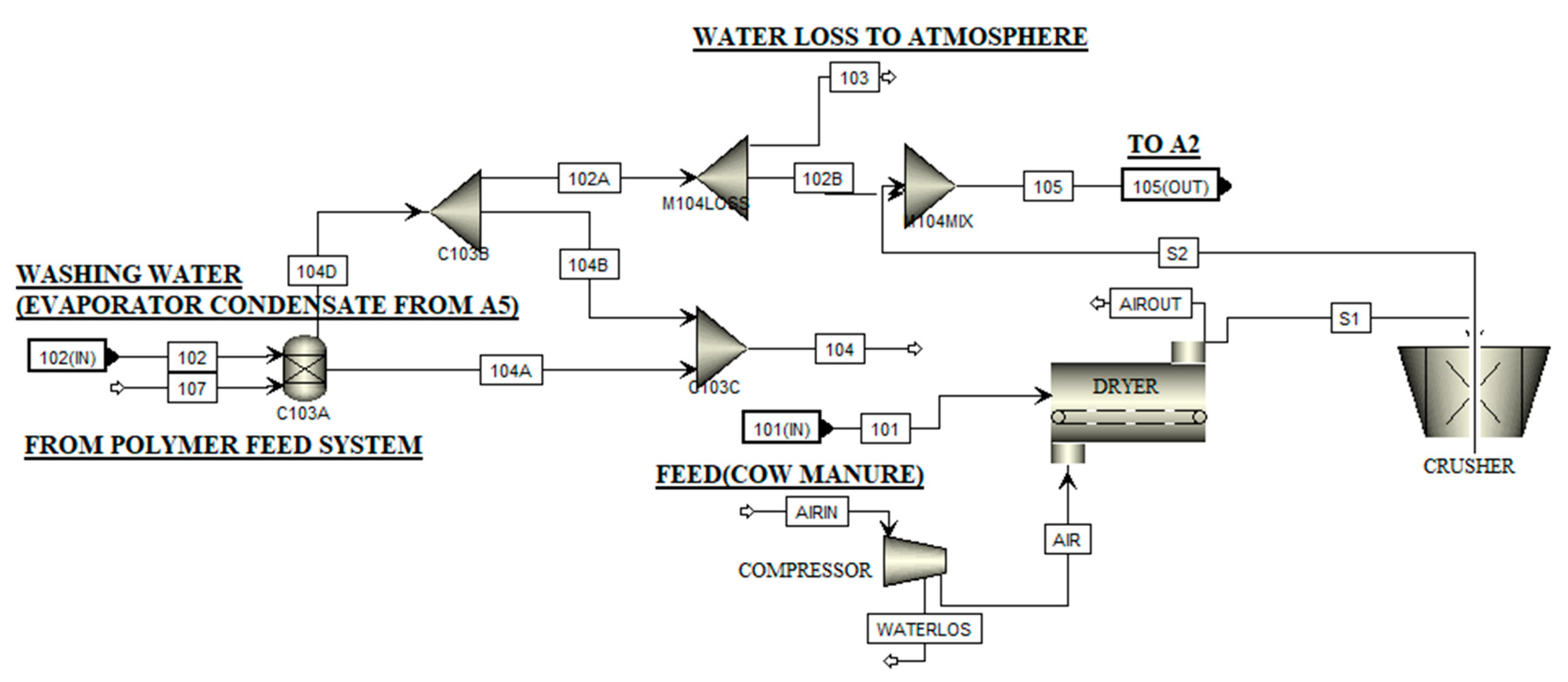
- To fulfill the bovine waste management needs, area A1 handled 2077 metric tons of dry bovine manure per day at scenario I, as opposed to the 2000 tons in the NREL model, when constructed at 100% capacity.
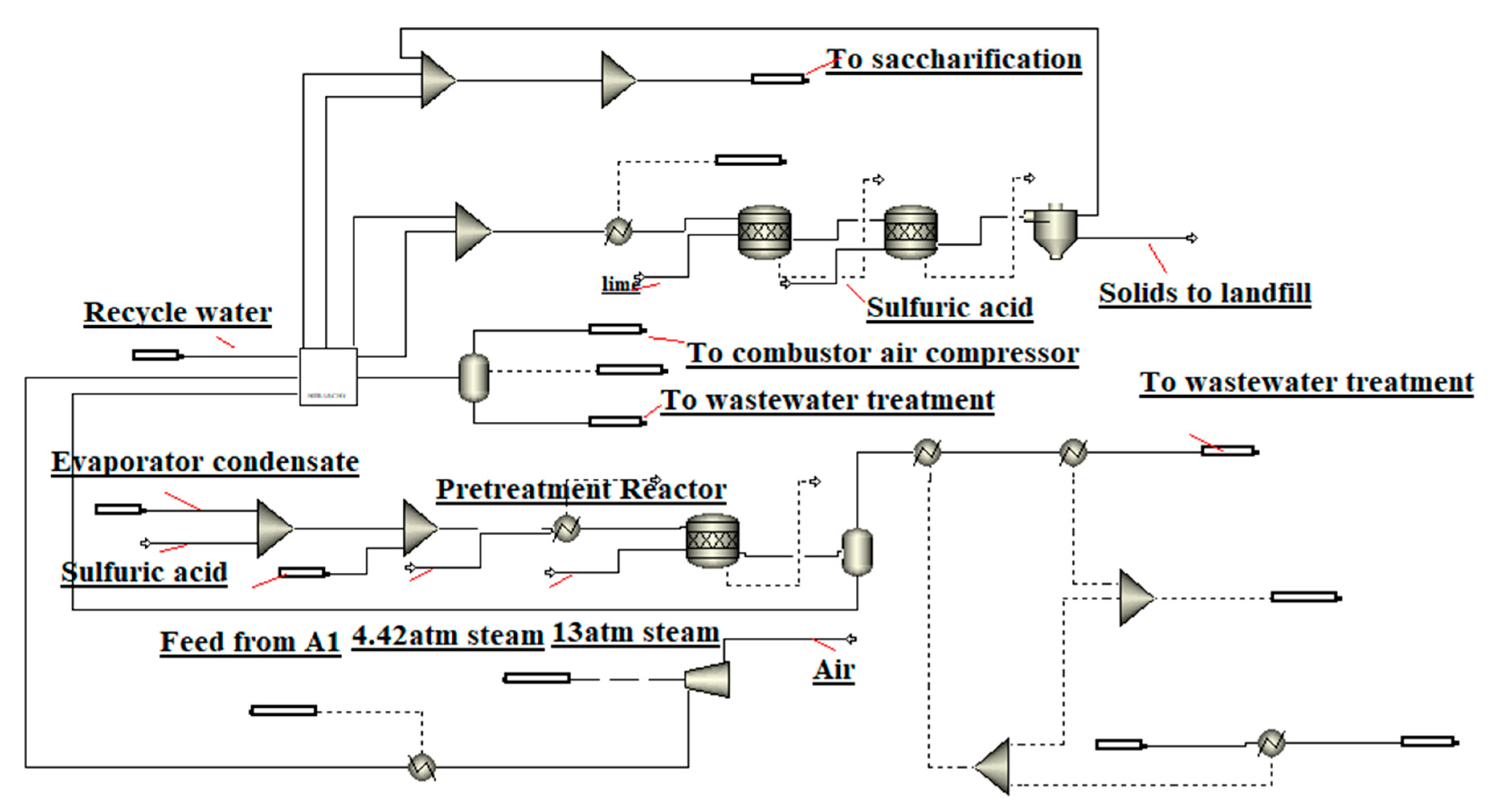
- In area A2, the dry dilute acid pretreatment method was applied with 8% of cow manure solids and 33% of dilute sulfuric acid solution (5% sulfuric acid in weight percentage). Solid–liquid separation using flash-cooling was required. This area included ammonia conditioning on liquid pretreatment hydrolysate, as per the NREL design.
- Simultaneous saccharification and fermentation: enzymatic hydrolysis at 30% (w/w) solid content and lactic acid fermentation using Bacillus coagulans DSM2314 were used in area A3, while separate ethanol fermentation and hydrolysis (SHF) at 20% solid content were used in the NREL 2011 design. Only one fermenter was needed to achieve the production capacity, instead of five as in the NREL design. The size changed depending on the scenario.
- Instead of the two-column ethanol distillation and one-column molecular sieve absorption in the NREL design, area A5 used centrifugation, precipitation, and separation [27].

| Parameter | Cow Manure Model | Reference |
|---|---|---|
| Pretreatment | ||
| Sulfuric acid loading | 1.25% per mg·g−1 dry biomass | [12] |
| Temperature | 120 °C | |
| Pressure (MPA) | 1 | |
| Residence time | 2 h | |
| Total solids loading | 8% (w/w) | |
| Detoxification | Ammonia conditioning | |
| SSAF | ||
| Strain | B. coagulans DSM2314 | |
| Temperature and residence time | 50 °C, 18 h (hydrolysis) | |
| 50 °C, 48 h (SSAF) | ||
| Total solids loading | 8% (w/w) | |
| Cellulases loading | 0.19 mL·g−1 | |
| Glucan conversion to glucose (%) | 90 | [28] |
| Ethanol and lactate yield from glucose (%) | 95 | |
| Ethanol and lactate yield from xylose (%) | 85 | [29] |
| Product recovery | 92% | [27] |
| Final product concentration (%) | 88% (w/w) lactic acid | [10] |
2.3.2. Front-End Operations
2.3.3. Pretreatment
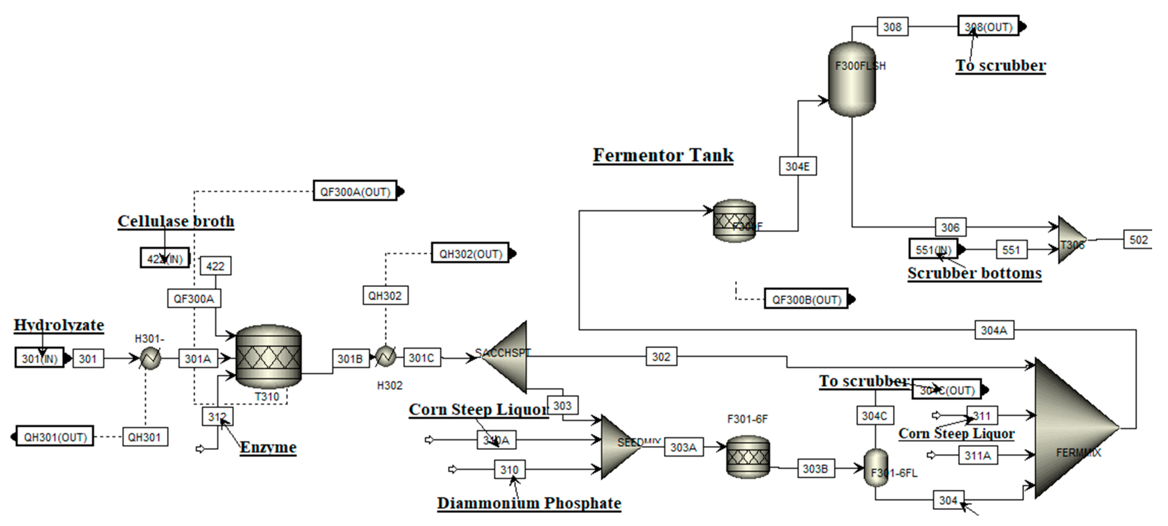
2.3.4. Saccharification and Fermentation
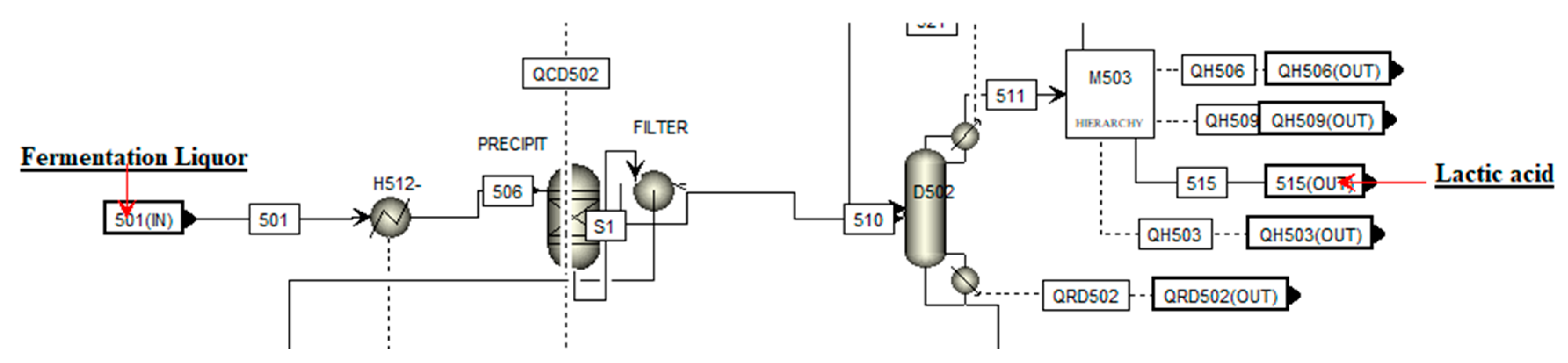
2.3.5. Lactic Acid Recovery
2.4. Economic Assessment
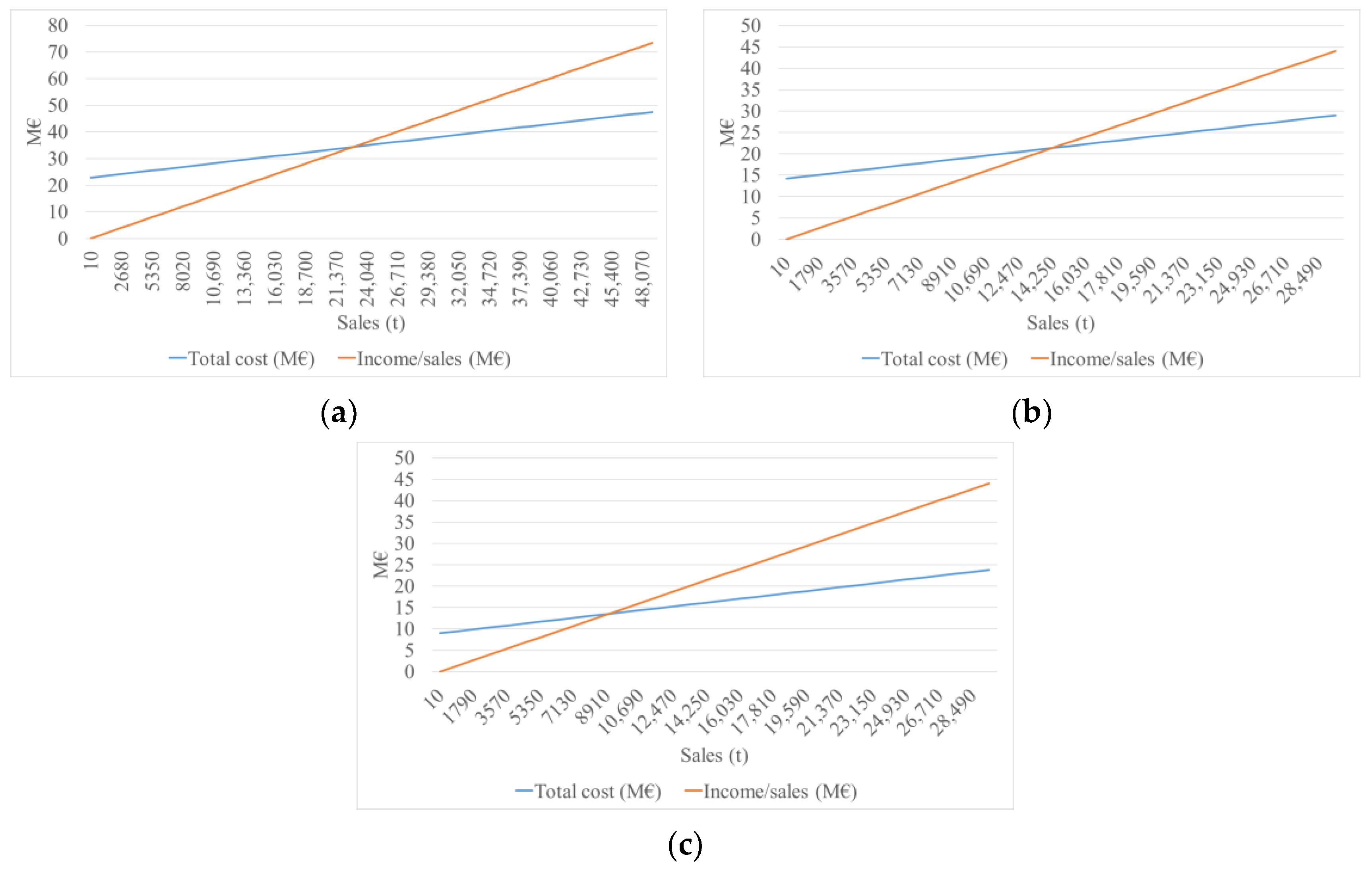
2.5. Sensitivity Analysis and Break-Even Point
3. Results and Discussion
3.1. Mass Balance
3.2. Capital Cost
3.3. Operation Cost
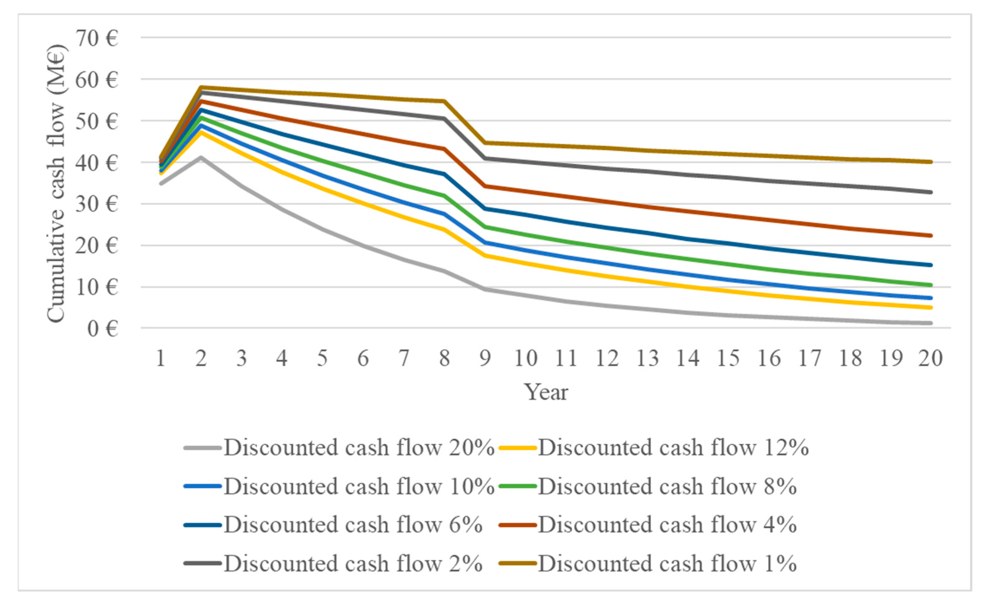
3.4. Revenue and Profitability Analysis
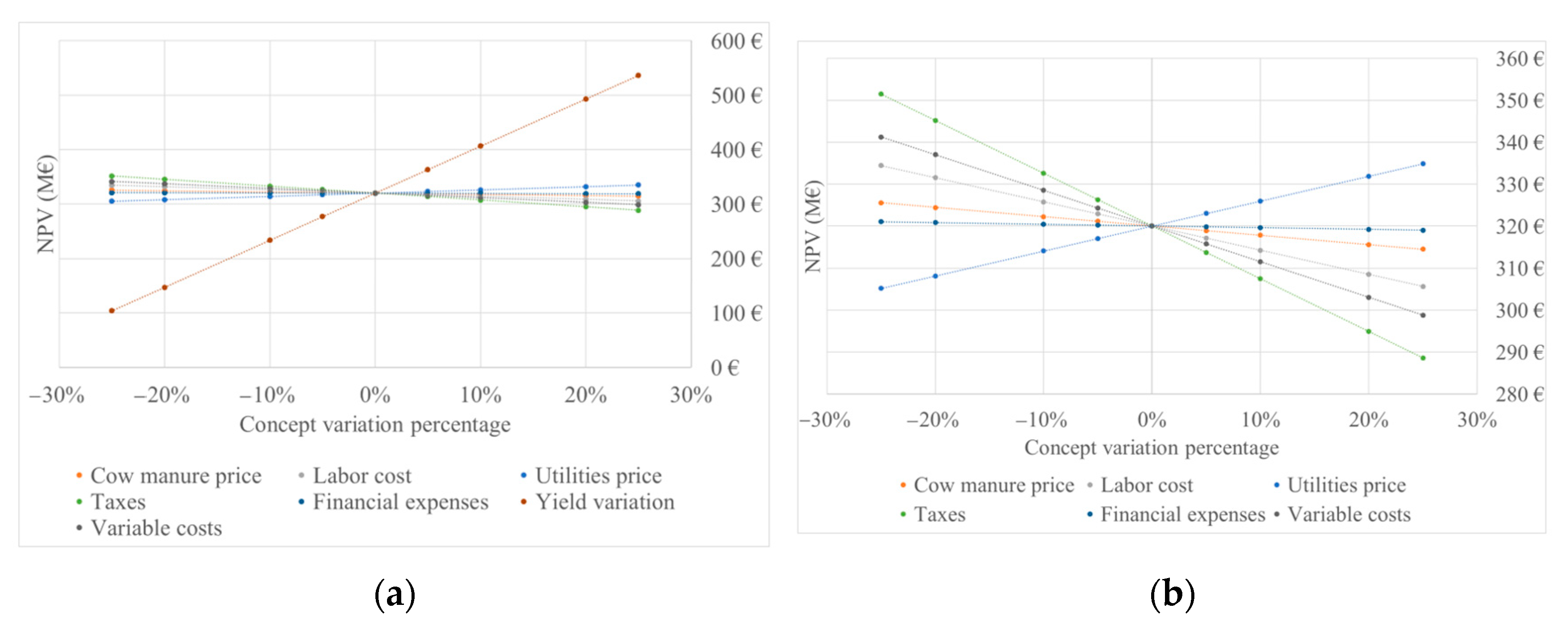
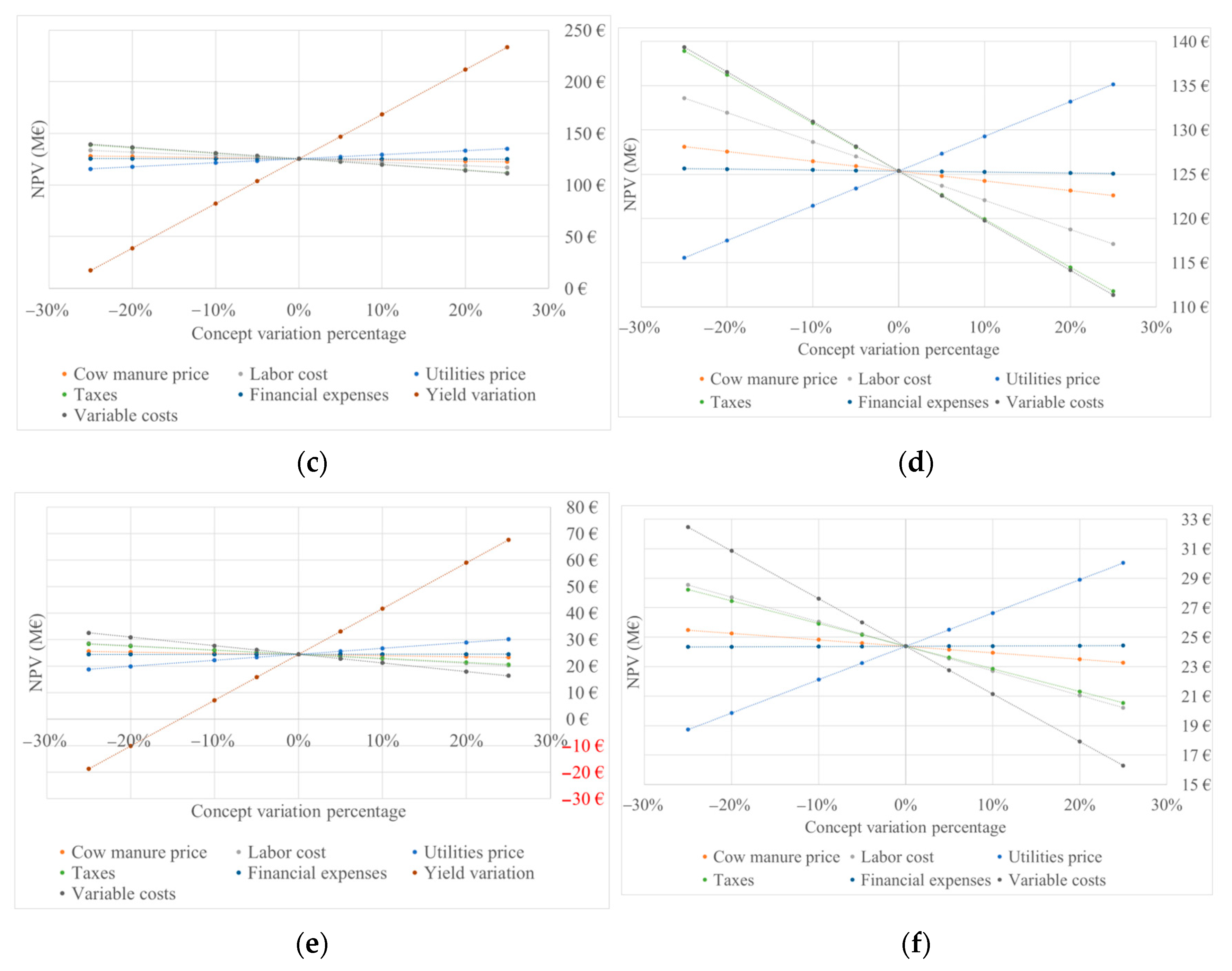
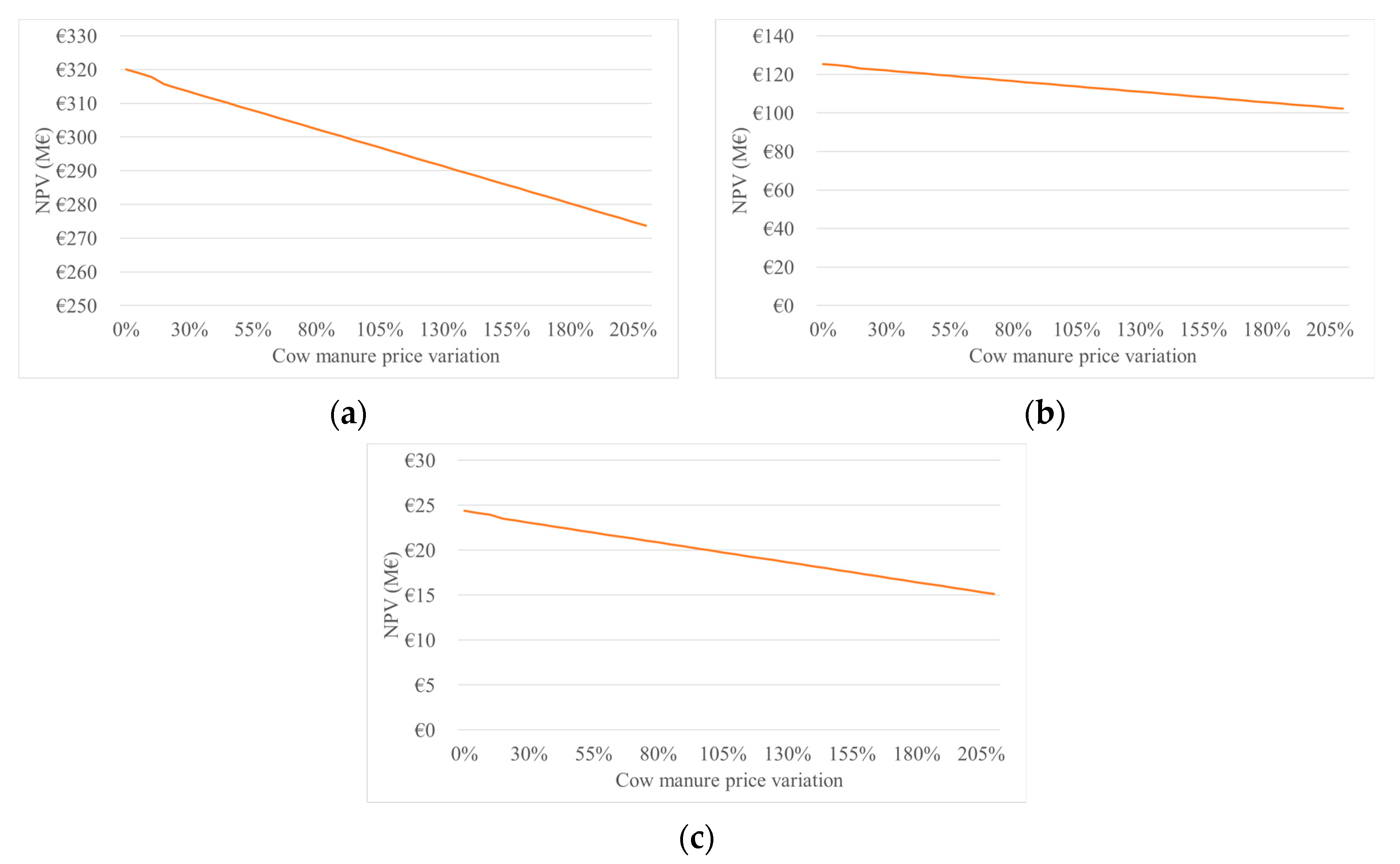
3.5. Sensitivity Analysis and Break-Even Point
4. Conclusions
Author Contributions
Funding
Institutional Review Board Statement
Informed Consent Statement
Data Availability Statement
Acknowledgments
Conflicts of Interest
References
- Ghaffar, T.; Irshad, M.; Anwar, Z.; Aqil, T.; Zulifqar, Z.; Tariq, A.; Kamran, M.; Ehsan, N.; Mehmood, S. Recent trends in lactic acid biotechnology: A brief review on production to purification. J. Radiat. Res. Appl. Sci. 2014, 7, 222–229. [Google Scholar] [CrossRef]
- Farooq, U.; Muhammad Anjum, F.; Zahoor, T.; Sajjad-Ur-Rahman; Atif Randhawa, M.; Ahmed, A.; Akram, K. Optimization of lactic acid production from cheap raw material: Sugarcane molasses. Pak. J. Bot. 2012, 44, 333–338. [Google Scholar]
- Wee, Y.J.; Kim, J.N.; Ryu, H.W. Biotechnological production of lactic acid and its recent applications. Food Technol. Biotechnol. 2006, 44, 163–172. [Google Scholar]
- Eurostat, “Production of Meat: Cattle”. 2022. Available online: https://ec.europa.eu/eurostat/databrowser/view/tag00044/default/table?lang=en (accessed on 1 July 2023).
- Gao, C.; Ma, C.; Xu, P. Biotechnological routes based on lactic acid production from biomass. Biotechnol. Adv. 2011, 29, 930–939. [Google Scholar] [CrossRef] [PubMed]
- Bai, D.; Zhao, X.-M.; Li, X.; Xu, S. Strain improvement of Rhizopus oryzae for over-production of l(+)-lactic acid and metabolic flux analysis of mutants. Biochem. Eng. J. 2004, 18, 41–48. Available online: https://api.semanticscholar.org/CorpusID:83839090 (accessed on 1 April 2004). [CrossRef]
- Castro-Aguirre, E.; Iñiguez-Franco, F.; Samsudin, H.; Fang, X.; Auras, R. Poly(lactic acid)—Mass production, processing, industrial applications, and end of life. Adv. Drug Deliv. Rev. 2016, 107, 333–366. [Google Scholar] [CrossRef] [PubMed]
- Garrido, R.; Cabeza, L.F.; Falguera, V.; Navarro, O.P. Potential Use of Cow Manure for Poly(Lactic Acid) Production. Sustainability 2022, 14, 16753. [Google Scholar] [CrossRef]
- Humbird, A.A.D.; Davis, R.; Tao, L.; Kinchin, C.; Hsu, D. Process Design; National Renewable Energy Laboratory: Golden, CO, USA, 2011. [Google Scholar] [CrossRef]
- Li, Y.; Bhagwat, S.S.; Cortés-Peña, Y.R.; Ki, D.; Rao, C.V.; Jin, Y.-S.; Guest, J.S. Sustainable Lactic Acid Production from Lignocellulosic Biomass. ACS Sustain. Chem. Eng. 2021, 9, 1341–1351. [Google Scholar] [CrossRef]
- Abedi, E.; Hashemi, S.M.B. Lactic acid production—Producing microorganisms and substrates sources-state of art. Heliyon 2020, 6, e04974. [Google Scholar] [CrossRef]
- Garrido, R.; Falguera, V.; Navarro, O.P.; Solares, A.A.; Cabeza, L.F. Lactic Acid Production from Cow Manure: Experimental Process Conditions Analysis. Fermentation 2023, 9, 604. [Google Scholar] [CrossRef]
- Amé, P. French Livestock Genetics and Territories. 2011. Available online: https://www.icar.org/wp-content/uploads/2015/09/Livestock-in-France_Philippe-AME.pdf (accessed on 11 July 2023).
- Department of Climate Action. Number of Holdings and Capacity. 2021. Available online: https://agricultura.gencat.cat/ca/departament/estadistiques/ramaderia/nombre-explotacions-capacitat/ (accessed on 11 July 2023).
- European Parliamentary Research Service. European Union Beef Sector: Main Features, Challenges and Prospects; European Parliamentary Research Service: Brussels, Belgium, 2022. [Google Scholar]
- D’Alcarras, A. Supporting the Strategic Planning of the Biolab Baix Segre. Project: Biovalue; Generalitat de Catalunya: Alcarras, Spain, 2019. [Google Scholar]
- Statista. Number of Cattle Worldwide from 2012 to 2023 (in Million Head). Farming, 2023. Available online: https://www.statista.com/statistics/263979/global-cattle-population-since-1990/ (accessed on 11 July 2023).
- de Haan, C.; Steinfeld, H.; Gerber, P.J.; Wassenaar, T.; Castel, V.; Rosales, M. Livestock’s Long Shadow: Environmental Issues and Options; FAO: Rome, Italy, 2006. [Google Scholar]
- Davis, J. Agricultural Price Volatility and Its Impact on Government and Farmers: A Few Observations. 2011. Available online: https://www.oecd.org/swac/events/48215044.pdf (accessed on 7 July 2023).
- Huffstutter, B.F.P.J.; Polansek, T. Cow Manure Price. Reuters, 2022. Available online: https://www.reuters.com/world/us/us-manure-is-hot-commodity-amid-commercial-fertilizer-shortage-2022-04-06/ (accessed on 22 May 2023).
- Wresta, A.; Andriani, D.; Saepudin, A.; Sudibyo, H. Economic analysis of cow manure biogas as energy source for electricity power generation in small scale ranch. Energy Procedia 2015, 68, 122–131. [Google Scholar] [CrossRef]
- Leip, A.; Ledgard, S.; Uwizeye, A.; Palhares, J.C.; Aller, M.F.; Amon, B.; Binder, M.; Cordovil, C.M.; De Camillis, C.; Dong, H.; et al. The value of manure—Manure as co-product in life cycle assessment. J. Environ. Manag. 2019, 241, 293–304. [Google Scholar] [CrossRef] [PubMed]
- Ghafoori, E.; Flynn, P.; Feddes, J. Pipeline vs. truck transport of beef cattle manure. Biomass Bioenergy 2007, 31, 168–175. [Google Scholar] [CrossRef]
- Green, R.H.; Perry, D.W. Perry’s Chemical Engineering Handbook; The McGraw-Hill Companies Inc.: New York, NY, USA, 2008. [Google Scholar]
- Tech, A. Aspen Plus; Aspen Technology Inc.: Bedford, MA, USA, 2023; Available online: https://www.aspentech.com/en/products/engineering/aspen-plus (accessed on 11 July 2023).
- Nakajima, S.; Conforti, M.; Rubbia, S. Introduction to TPM: Total Productive Maintenance; Productivity Press, Inc.: New York, NY, USA, 1997. [Google Scholar]
- Komesu, A.; Maciel, M.R.W.; Filho, R.M. Separation and purification technologies for lactic acid—A brief review. BioResources 2017, 12, 6885–6901. [Google Scholar] [CrossRef]
- Benavides, P.; Zare‘-Mehrjerdi, O.; Lee, U. Life-Cycle Analysis of Bioproducts and Their Conventional Counterparts in GREETTM Energy Systems Division. 2019. Available online: www.anl.gov (accessed on 11 July 2023).
- Abdel-Rahman, M.A.; Tashiro, Y.; Zendo, T.; Hanada, K.; Shibata, K.; Sonomoto, K. Efficient homofermentative L-(+)-Lactic acid production from xylose by a novel lactic acid bacterium, Enterococcus mundtii QU 25. Appl. Environ. Microbiol. 2011, 77, 1892–1895. [Google Scholar] [CrossRef] [PubMed]
- Campos, E.; Palatsi, J.; Illa, J.; Magrí, A.; Solé, F.; Flotats, X. Guide to the Treatment of Livestock Injections. 2004. Available online: http://www.arc-cat.net/es/altres/purins/guia/pdf/guia_dejeccions.pdf (accessed on 7 July 2023).
- Lemões, J.S.; e Silva, C.F.L.; Avila, S.P.F.; Montero, C.R.S.; dos Anjos e Silva, S.D.; Samios, D.; Peralba, M.D.C.R. Chemical pretreatment of Arundo donax L. for second-generation ethanol production. Electron. J. Biotechnol. 2018, 31, 67–74. [Google Scholar] [CrossRef]
- Abdel-Rahman, M.A.; Tashiro, Y.; Sonomoto, K. Lactic acid production from lignocellulose-derived sugars using lactic acid bacteria: Overview and limits. J. Biotechnol. 2011, 156, 286–301. [Google Scholar] [CrossRef]
- van der Pol, E.C.; Eggink, G.; Weusthuis, R.A. Production of l(+)-lactic acid from acid pretreated sugarcane bagasse using Bacillus coagulans DSM2314 in a simultaneous saccharification and fermentation strategy. Biotechnol. Biofuels 2016, 9, 248. [Google Scholar] [CrossRef]
- Datta, R.; Henry, M. Lactic acid: Recent advances in products, processes and technologies—A review. J. Chem. Technol. Biotechnol. 2006, 81, 1119–1129. [Google Scholar] [CrossRef]
- Abdel-Rahman, M.A.; Sonomoto, K. Opportunities to overcome the current limitations and challenges for efficient microbial production of optically pure lactic acid. J. Biotechnol. 2016, 236, 176–192. [Google Scholar] [CrossRef]
- Trindade, M.C. Estudo da Recuperação de Ácido Lático Proveniente do soro de Queijo Pela Técnica de Membranas Líquidas Surfatantes; Universidade Federal de Minas Gerais: Belo Horizonte, Brazil, 2002. [Google Scholar]
- Pereira, A.J.G. Purificação do Ácido Láctico Através de Extração Líquido-líquido; Universidade Estadual de Campinas: Campinas, Brazil, 1991. [Google Scholar]
- Chen, X.; Tao, L.; Shekiro, J.; Mohaghaghi, A.; Decker, S.; Wang, W.; Smith, H.; Park, S.; Himmel, M.E.; Tucker, M. Improved ethanol yield and reduced minimum ethanol selling price (MESP) by modifying low severity dilute acid pretreatment with deacetylation and mechanical refining: 1 Experimental. Biotechnol. Biofuels 2012, 5, 60. [Google Scholar] [CrossRef] [PubMed]
- Åkerberg, C.; Zacchi, G. An economic evaluation of the fermentative production of lactic acid from wheat flour. Bioresour. Technol. 2000, 75, 119–126. [Google Scholar] [CrossRef]
- Salary.com. Salaries. 2023. Available online: https://www.salary.com/research/es-salary/alternate/plant-production-operations-manager-salary/es (accessed on 26 March 2023).
- Statista. Evolution of the Annual Average of the Exchange Rate of the Euro to the US Dollar from 1999 to 2022. 2023. Available online: https://es.statista.com/estadisticas/606660/media-anual-de-la-tasa-de-cambio-de-euro-a-dolar-estadounidense/ (accessed on 3 May 2023).
- Garrett, D.E. Chemical Engineering Economics; Springer: Dordrecht, The Netherlands, 1989. [Google Scholar]
- Peters, R.; Timmerhaus, M.; West, K. Plant Design and Economics for Chemical Engineers, 4th ed.; McGraw-Hill International: Boston, MA, USA, 2003. [Google Scholar]
- Peters, M.S.; Timmerhaus, K.D.; West, R.E. Plant Design and Economics for Chemical Engineers Equipment Web. January, 2002. Available online: http://www.mhhe.com/engcs/chemical/peters/data/ce.html (accessed on 16 June 2023).
- Llano, T.; Arce, C.; Gallart, L.E.; Perales, A.; Coz, A. Techno-Economic Analysis of Macroalgae Biorefineries: A Comparison between Ethanol and Butanol Facilities. Fermentation 2023, 9, 340. [Google Scholar] [CrossRef]
- Dziekońska-Kubczak, U.; Berłowska, J.; Dziugan, P.; Patelski, P.; Balcerek, M.; Pielech-Przybylska, K.; Robak, K. Two-Stage Pretreatment to Improve Saccharification of Oat Straw and Jerusalem Artichoke Biomass. Energies 2019, 12, 1715. [Google Scholar] [CrossRef]
- Trakulvichean, S.; Chaiprasert, P.; Otmakhova, J.; Songkasiri, W. Comparison of fermented animal feed and mushroom growth media as two value-added options for waste Cassava pulp management. Waste Manag. Res. 2017, 35, 1210–1219. [Google Scholar] [CrossRef] [PubMed]
- Agencia Tributiaria. Machinery Amortization Table. 2023. Available online: https://sede.agenciatributaria.gob.es/Sede/ayuda/manuales-videos-folletos/manuales-practicos/folleto-actividades-economicas/3-impuesto-sobre-renta-personas-fisicas/3_5-estimacion-directa-simplificada/3_5_4-tabla-amortizacion-simplificada.html (accessed on 1 May 2023).
- Agencia Tributaria. Spain Corporate Tax. Manual Práctico de Sociedades 2022. 2022. Available online: https://sede.agenciatributaria.gob.es/Sede/ayuda/manuales-videos-folletos/manuales-practicos/manual-sociedades-2022/capitulo-01-cuestiones-generales/que-impuesto-sobre-sociedades.html (accessed on 19 June 2023).
- Davis, R.E.; Grundl, N.J.; Tao, L.; Biddy, M.J.; Tan, E.C.; Beckham, G.T.; Humbird, D.; Thompson, D.N.; Roni, M.S. Process Design and Economics for the Conversion of Lignocellulosic Biomass to Hydrocarbon Fuels and Coproducts: 2018 Biochemical Design Case Update Biochemical Deconstruction and Conversion of Biomass to Fuels and Products via Integrated Biorefinery Pathways; National Renewable Energy Lab. (NREL): Golden, CO, USA, 2018. [Google Scholar]
- Ulrich, G.D. A Guide to Chemical Engineering Process Design and Economics; Wiley: New York, NY, USA, 1984. [Google Scholar]
- Aqualia. Lleida Municipal Water. 2023. Available online: https://www.aqualia.com/web/servicio-municipal-de-agua-tarifas/lleida# (accessed on 20 June 2023).
- Jerry, J.E.M.; Weygandt, J.; Kimmel, P.D. Financial Accounting; Wiley: Hoboken, NJ, USA, 2022. [Google Scholar]
- Made-in-China. Lactic Acid Pricing China. Available online: https://www.made-in-china.com/products-search/hot-china-products/lactic_acid_price.html (accessed on 22 May 2023).
- Broadie, M.; Chernov, M.; Sundaresan, S. Optimal debt and equity values in the presence of chapter 7 and chapter 11. J. Financ. 2007, 62, 1341–1377. [Google Scholar] [CrossRef]
- Vink, E.T.H.; Davies, S. Life Cycle Inventory and Impact Assessment Data for 2014 IngeoTM polylactide production. Ind. Biotechnol. 2015, 11, 167–180. [Google Scholar] [CrossRef]
- Min, D.J.; Choi, K.H.; Chang, Y.K.; Kim, J.H. Effect of operating parameters on precipitation for recovery of lactic acid from calcium lactate fermentation broth. Korean J. Chem. Eng. 2011, 28, 1969–1974. [Google Scholar] [CrossRef]
- de Estadística, I.N. Calculation of Variations of the Consumer Price Index (CPI System Base 2021). 2023. Available online: https://www.ine.es/varipc/verVariaciones.do;jsessionid=66885B9223388EB826AD3BC7F0546DAD.varipc03?idmesini=3&anyoini=2000&idmesfin=3&anyofin=2023&ntipo=1&enviar=Calcular (accessed on 30 April 2023).
- Mupondwa, E.; Li, X.; Boyetchko, S.; Hynes, R.; Geissler, J. Technoeconomic analysis of large scale production of pre-emergent Pseudomonas fluorescens microbial bioherbicide in Canada. Bioresour. Technol. 2015, 175, 517–528. [Google Scholar] [CrossRef]
- Koutinas, A.A.; Yepez, B.; Kopsahelis, N.; Freire, D.M.; de Castro, A.M.; Papanikolaou, S.; Kookos, I.K. Techno-economic evaluation of a complete bioprocess for 2,3-butanediol production from renewable resources. Bioresour. Technol. 2016, 204, 55–64. [Google Scholar] [CrossRef]
- Infojobs. Infojobs Salaries. 2023. Available online: https://salarios.infojobs.net/ (accessed on 20 April 2023).
- Dimian, A.C.; Bildea, C.S.; Kiss, A.A. Chapter 19—Economic Evaluation of Projects. In Integrated Design and Simulation of Chemical Processes; Dimian, A.C., Bildea, C.S., Kiss, A.A., Eds.; Elsevier: Amsterdam, The Netherlands, 2014; Volume 35, pp. 717–755. [Google Scholar]
- Birken, E.G. Return of Investment. Forbes, 2023. Available online: https://www.forbes.com/advisor/investing/roi-return-on-investment/ (accessed on 31 July 2023).
- González, M.I.; Álvarez, S.; Riera, F.; Álvarez, R. Economic evaluation of an integrated process for lactic acid production from ultrafiltered whey. J. Food Eng. 2007, 80, 553–561. [Google Scholar] [CrossRef]
- Sikder, J.; Roy, M.; Dey, P.; Pal, P. Techno-economic analysis of a membrane-integrated bioreactor system for production of lactic acid from sugarcane juice. Biochem. Eng. J. 2012, 63, 81–87. [Google Scholar] [CrossRef]
- Liu, G.; Sun, J.; Zhang, J.; Tu, Y.; Bao, J. High titer l -lactic acid production from corn stover with minimum wastewater generation and techno-economic evaluation based on Aspen plus modeling. Bioresour. Technol. 2015, 198, 803–810. [Google Scholar] [CrossRef] [PubMed]
- Vantage. Lactic Acid Market Size USD 4.03 Billion by 2030. 2023. Available online: https://www.vantagemarketresearch.com/industry-report/lactic-acid-market-1150 (accessed on 5 June 2023).
| Stable | Hemicellulose (%) | Cellulose (%) | Lignin (%) | Ash (%) | Humidity (%) |
|---|---|---|---|---|---|
| Manure heap A * | 27.3 | 24.5 | 3.8 | 17.69 | 2.32 |
| Manure heap B * | 26.3 | 25 | 3.8 | 18.85 | 2.5 |
| Farm 1A | 28.3 | 23.4 | 3.5 | 18.04 | 2.32 |
| Farm 1B | 30.2 | 21.7 | 3.1 | 17.43 | 2.11 |
| Farm 2A | 28.4 | 23.6 | 4.1 | 17.13 | 2.76 |
| Farm 2B | 28.3 | 22.9 | 5.3 | 16.5 | 2.23 |
| Average | 28.1 | 23.5 | 3.9 | 17.6 | 2.4 |
| Parameter | Scenario I | Scenario II | Scenario III |
|---|---|---|---|
| Plant capacity (t) Cow manure per year | 1,579,328 | 947,597 | 315,866 |
| Capacity treated (%) | 100 | 50 | 20 |
| Parameter | Scenario I | Scenario II | Scenario III |
|---|---|---|---|
| Step | Quantity (t) | Quantity (t) | Quantity (t) |
| Raw material | 1,579,328 | 789,664 | 315,866 |
| Dry raw material | 758,077 | 379,039 | 151,615 |
| Fermented LA | 109,723 | 54,861 | 21,945 |
| LA recovered (92%) | 100,945 | 60,567 | 20,189 |
| Process Area | Percentage | Installation Factor Average | Scenario I Installed Cost (EUR) | Scenario II Installed Cost (EUR) | Scenario III Installed Cost (EUR) |
|---|---|---|---|---|---|
| A1: Feedstock handling | NA | 1.7 | 12,095,436 | 7,980,012 | 4,605,105 |
| A2: Pretreatment | NA | 1.9 | 12,821,690 | 8,459,160 | 4,881,612 |
| A3: SSAF | NA | 1.9 | 7,846,272 | 5,176,609 | 2,987,317 |
| A4: Enzyme production | NA | 1.9 | 17,990,074 | 11,869,022 | 6,849,375 |
| A5: Recovery | NA | 2.2 | 19,000,203 | 12,535,459 | 7,233,962 |
| A6: Wastewater | NA | 1 | 17,820,506 | 11,757,150 | 6,784,815 |
| A7: Storage | NA | 2.1 | 3,637,493 | 2,399,850 | 1,384,906 |
| A8: Boiler | NA | 2.1 | 17,220,927 | 11,361,575 | 6,556,537 |
| A9: Utilities | NA | 2.2 | 474,476 | 313,037 | 180,648 |
| Totals | 108,907,077 | 71,851,875 | 41,464,277 | ||
| Warehouse | 4.00% | of inside battery limits (ISBL) | 4,356,283 | 2,874,075 | 1,658,571 |
| Site development | 9.00% | of ISBL | 9,801,637 | 6,466,669 | 3,731,785 |
| Additional piping | 4.50% | of ISBL | 4,900,818 | 3,233,334 | 1,865,892 |
| Total direct costs (TDC) | 127,965,815.63 | 84,425,953.02 | 48,720,525.79 | ||
| Proratable expenses | 10.00% | of TDC | 10,890,708 | 7,185,187 | 4,146,428 |
| Field expenses | 10.00% | of TDC | 10,890,708 | 7,185,187 | 4,146,428 |
| Home office and construction fee | 20.00% | of TDC | 21,781,415 | 14,370,375 | 8,292,855 |
| Project contingency | 10.00% | of TDC | 10,890,708 | 7,185,187 | 4,146,428 |
| Other costs (start-up, permits, etc.) | 10.00% | of TDC | 10,890,708 | 7,185,187.49 | 4,146,427.73 |
| Total Indirect Costs | 65,344,246 | 43,111,125 | 24,878,566 | ||
| Fixed Capital Investment (FCI) | 193,310,062 | 127,537,078 | 73,599,092 | ||
| Working capital | 5.00% | of FCI | 9,665,503 | 6,376,854 | 3,679,955 |
| Total Capital Investment (TCI) | 202,975,565 | 133,913,932 | 77,279,047 | ||
| Scenario I | Scenario II | Scenario III | |||||||||
|---|---|---|---|---|---|---|---|---|---|---|---|
| Process Area | Stream Description | Cost (EUR·t−1) | Usage (kg·h−1) | EUR/h (2023) | MEUR/y (2023 EUR) | Usage (kg·h−1) | EUR/h (2023) | MEUR/y (2023 EUR) | Usage (kg·h−1) | EUR/h (2023) | MEUR/y (2023 EUR) |
| Raw materials | |||||||||||
| A1 | Feedstock (wet) | 56.92 | 104,167 | 520.84 | 4.41 | 68,725 | 343.62 | 2.91 | 39,659.58 | 198.30 | 1.68 |
| A2 | Sulfuric acid, 93% | 98.99 | 1981 | 196.09 | 1.66 | 1307 | 129.37 | 1.09 | 754.23 | 74.66 | 0.63 |
| Ammonia | 494.94 | 1051 | 520.18 | 4.40 | 693 | 343.19 | 2.90 | 400.15 | 198.05 | 1.68 | |
| A3 | Corn steep liquor | 62.69 | 1158 | 72.60 | 0.61 | 764 | 47.90 | 0.41 | 440.89 | 27.64 | 0.23 |
| Diammonium phosphate | 1088.88 | 142 | 154.62 | 1.31 | 93.69 | 102.01 | 0.86 | 54.06 | 58.87 | 0.50 | |
| Sorbitol | 1242.86 | 44 | 54.69 | 0.5 | 29.03 | 36.08 | 0.3 | 16.75 | 20.82 | 0.2 | |
| A4 | Glucose | 640.35 | 2418 | 1548.36 | 13.1 | 1595 | 1021.54 | 8.6 | 920.61 | 589.51 | 5.0 |
| Corn steep liquor | 62.69 | 164 | 10.28 | 0.1 | 108.1996 | 6.78 | 0.1 | 62.44 | 3.91 | 0.03 | |
| Ammonia | 494.94 | 115 | 56.92 | 0.5 | 75.87 | 37.55 | 0.3 | 43.78 | 21.67 | 0.2 | |
| Host nutrients | 906.43 | 67 | 60.73 | 0.5 | 44.20 | 40.07 | 0.3 | 25.51 | 23.12 | 0.2 | |
| Sulfur dioxide | 335.30 | 16 | 5.36 | 0.045 | 10.56 | 3.54 | 0.03 | 6.09 | 2.04 | 0.02 | |
| A5 | Methanol | 191.55 | 15 | 2.87 | 0.02 | 9.90 | 1.90 | 0.02 | 5.71 | 1.094 | 0.01 |
| A6 | Caustic | 164.98 | 2252 | 371.53 | 3.1 | 1485.77 | 245.12 | 2.1 | 857.41 | 141.45 | 1.2 |
| A8 | Boiler chems | 5511.98 | 1 | 5.51 | 0.0 | 0.66 | 3.64 | 0.0 | 0.38 | 2.10 | 0.02 |
| FGD lime | 219.97 | 895 | 196.88 | 1.7 | 590.48 | 129.89 | 1.1 | 340.75 | 74.96 | 0.6 | |
| A9 | Cooling tower chems | 3303.29 | 2 | 6.61 | 0.1 | 1.32 | 4.36 | 0.04 | 0.76 | 2.52 | 0.02 |
| Makeup water | 0.28 | 147,140 | 41.16 | 0.3 | 97,076.20 | 27.15 | 0.2 | 56,020.73 | 15.67 | 0.1 | |
| Subtotal | 3825.23 | 32.4 | 2523.71 | 21.4 | 1456.38 | 12.3 | |||||
| Waste disposal | |||||||||||
| A8 | Disposal of ash | 5725 | 200.94 | 1.70 | 3777 | 132.57 | 1.12 | 77 | 2.69 | 0.02 | |
| Subtotal | 200.94 | 1.70 | 132.57 | 1.12 | 2.69 | 0.02 | |||||
| Byproducts and credits | |||||||||||
| Grid electricity (KW) | 12,797 | 639.85 | 5.41 | 8443 | 422.14 | 3.57 | 4872 | 243.61 | 2.06 | ||
| Area 100 electricity | 859 | 42.95 | 0.36 | 567 | 28.34 | 0.24 | 327 | 16.35 | 0.14 | ||
| Subtotal | 682.8 | 5.776 | 450.480 | 3.811 | 259.963 | 2.20 | |||||
| Total variable operating costs | 4708.97 | 39.84 | 3106.76 | 26.28 | 1719.03 | 14.54 | |||||
| Labor and Supervision | |||||||
|---|---|---|---|---|---|---|---|
| Scenario I | Scenario II | Scenario III | |||||
| Position | Salary (EUR) | Positions | Total cost (EUR) | Positions | Total cost (EUR) | Positions | Total cost (EUR) |
| Plant manager | 141,569 | 1 | 141,569 | 1 | 141,569 | 0 | 0 |
| Plant engineer | 67,414 | 2 | 134,828 | 1 | 67,414 | 1 | 67,414 |
| Maintenance supervisor | 54,894 | 1 | 54,894 | 1 | 54,894 | 1 | 54,894 |
| Maintenance technician | 38,522 | 12 | 462,264 | 8 | 308,176 | 4 | 154,088 |
| Lab manager | 53,931 | 1 | 53,931 | 1 | 53,931 | 0 | 0 |
| Lab technician | 38,522 | 2 | 77,044 | 2 | 77,044 | 1 | 38,522 |
| Lab tech-enzyme | 38,771 | 2 | 77,542 | 1 | 38,771 | 1 | 38,771 |
| Shift supervisor | 46,227 | 4 | 184,908 | 2 | 92,454 | 1 | 46,227 |
| Shift operators | 38,522 | 20 | 770,440 | 8 | 308,176 | 4 | 154,088 |
| Shift open-enzyme | 38,771 | 8 | 310,168 | 4 | 155,084 | 3 | 116,313 |
| Yard employees | 26,966 | 4 | 107,864 | 3 | 80,898 | 2 | 53,932 |
| Clerks and secretaries | 34,670 | 3 | 104,010 EUR | 2 | 69,340 | 1 | 34,670 |
| Total salaries (EUR) | 2,479,462 | 1,447,751 | 758,919 | ||||
| Labor burden (90%) (EUR) | 2,231,516 | 1,302,976 | 683,027 | ||||
| Other overhead | |||||||
| Maintenance of ISBL (%) | 3.00 | 3,838,974 | 2,532,779 | 1,461,616 | |||
| Property insurance of FCI (%) | 0.70 | 1,420,829 | 937,398 | 540,953 | |||
| Total fixed operating costs (EUR) | 7,739,265 | 4,917,927 | 2,761,488 | ||||
| Parameter | Scenario I | Scenario II | Scenario III |
|---|---|---|---|
| Cow manure plant capacity (t·year−1) | 1,579,328 | 789,664 | 315,866 |
| Design on-stream factor (346 days·year−1) | 0.95 | ||
| Feedstock | Cow manure | ||
| Feedstock price (EUR·t−1) | 5 | ||
| Main products | Lactic Acid | ||
| Selling price (EUR·kg−1) | 1.5 | ||
| Total capital investment (MEUR) | 202.98 | 133.91 | 77.28 |
| Operation cost (MEUR·year−1) | 50.85 | 25.40 | 10.17 |
| Revenues (MEUR/year) after amortization | 48.85 | 23.20 | 8.30 |
| LA batch size (t) | 553.1 | 276.6 | 110.6 |
| Yield (%) | 33.3 | ||
| OEE (%) | 85 | ||
| Unit production cost (EUR·kg−1) | 0.748 | 0.809 | 0.924 |
| Payback time (years) | 3 | 4 | 8 |
| IRR (After Taxes) | 26% | 20% | 12% |
| NPV (at 8% Interest) (MEUR) | 320 | 125 | 24 |
| ROI (%) | 16.66 | 9.94 | 3.42 |
| MSP (EUR·kg−1) | 0.945 | 1.070 | 1.289 |
| 20 t daily trucks (365 days) | 104 | 52 | 21 |
| Scenario I | Scenario II | Scenario III | |
|---|---|---|---|
| Variable | Variation | Variation | Variation |
| Cow manure price | 97% | 96% | 91% |
| Labor cost | 91% | 88% | 71% |
| Utilities price | 110% | 117% | 160% |
| Taxes | 82% | 80% | 73% |
| Financial expenses | 99% | 100% | 100% |
| Yield variation | 516% | 1347% | 447% |
| Variable costs | 88% | 80% | 50% |
Disclaimer/Publisher’s Note: The statements, opinions and data contained in all publications are solely those of the individual author(s) and contributor(s) and not of MDPI and/or the editor(s). MDPI and/or the editor(s) disclaim responsibility for any injury to people or property resulting from any ideas, methods, instructions or products referred to in the content. |
© 2023 by the authors. Licensee MDPI, Basel, Switzerland. This article is an open access article distributed under the terms and conditions of the Creative Commons Attribution (CC BY) license (https://creativecommons.org/licenses/by/4.0/).
Share and Cite
Garrido, R.; Cabeza, L.F.; Falguera, V. Lactic Acid Production from Cow Manure: Technoeconomic Evaluation and Sensitivity Analysis. Fermentation 2023, 9, 901. https://doi.org/10.3390/fermentation9100901
Garrido R, Cabeza LF, Falguera V. Lactic Acid Production from Cow Manure: Technoeconomic Evaluation and Sensitivity Analysis. Fermentation. 2023; 9(10):901. https://doi.org/10.3390/fermentation9100901
Chicago/Turabian StyleGarrido, Ricard, Luisa F. Cabeza, and Víctor Falguera. 2023. "Lactic Acid Production from Cow Manure: Technoeconomic Evaluation and Sensitivity Analysis" Fermentation 9, no. 10: 901. https://doi.org/10.3390/fermentation9100901