Adapting the Segment Anything Model for Plant Recognition and Automated Phenotypic Parameter Measurement

Abstract

Traditional phenotyping relies on experts visually examining plants for physical traits like size, color, or disease presence. Measurements are taken manually using rulers, scales, or color charts, with all data recorded by hand. This labor-intensive and time-consuming process poses a significant obstacle to the efficient breeding of new cultivars. Recent innovations in computer vision and machine learning offer potential solutions for accelerating the development of robust and highly effective plant phenotyping. This study introduces an efficient plant recognition framework that leverages the power of the Segment Anything Model (SAM) guided by Explainable Contrastive Language–Image Pretraining (ECLIP). This approach can be applied to a variety of plant types, eliminating the need for labor-intensive manual phenotyping. To enhance the accuracy of plant phenotype measurements, a B-spline curve is incorporated during the plant component skeleton extraction process. The effectiveness of our approach is demonstrated through experimental results, which show that the proposed framework achieves a mean absolute error (MAE) of less than 0.05 for the majority of test samples. Remarkably, this performance is achieved without the need for model training or labeled data, highlighting the practicality and efficiency of the framework.

1. Introduction

Plant phenotyping is an increasingly crucial aspect of agricultural research that help to effectively address global challenges related to food security, climate change, and sustainable agriculture [1]. It involves the detailed observation and precise measurement of plant traits, including growth patterns, crop yield, and resistance to various biological and environmental stresses like drought, pests, and diseases [2]. These traits are often complex and can be affected by the interplay between genetic factors and environmental conditions. Phenotyping data collection offers crucial understanding into how plants perform and adapt under varying environmental conditions. This information is essential for plant breeders, who use it to select plants with desirable characteristics for breeding programs [3]. The ultimate goal is to cultivate novel crop varieties that are resistant to diseases and capable of growing in challenging weather conditions, and more productive. Therefore, plant phenotyping plays an important role in food security and sustainable agriculture [3].

Previous studies have mainly relied on image-oriented measurement techniques to analyze phenotypic traits [4]. This process typically requires experts to physically examine the plants and record data on various traits like plant height, leaf area, and color [5]. The data are then used to determine the plant’s health, growth, and productivity [6]. Despite being time-consuming and prone to error, this manual process is accessible and cost-effective. It is therefore suitable for small-scale studies or field research where advanced phenotyping platforms are unavailable [7].

Recent advancements in plant phenotyping have involved the integration of computer vision (CV) and deep learning (DL), which holds great promise for accelerating crop improvement and ensuring global food security [8,9]. Such methods use advanced imaging techniques to capture images of plants, which are then analyzed using DL algorithms [10,11]. These algorithms allow accurate prediction of various plant traits, enabling high-throughput and non-destructive phenotyping. This approach significantly improves the speed and accuracy of data collection, allowing for the analysis of larger plant populations and more complex traits [12]. Furthermore, it reduces the need for manual intervention, thus minimizing potential errors and inconsistencies.

For example, Dang et al. presented a novel method for monitoring the growth of white radish, a globally consumed vegetable, using high-resolution images and a mathematical model [13]. The study utilized a mask region-based convolutional neural network (Mask-RCNN) model to recognize various radish components and automatically measure their biophysical properties, with an emphasis on minimizing the impact of light conditions. The automated method achieved an average accuracy of 96.2% compared to the manual method, indicating its effectiveness in quantifying phenotypic traits. In another study, Zhou et al. proposed Maize-IAS, a DL-based maize phenotyping analysis framework [14]. The system processes RGB images of maize and offers a user-friendly interface and swift computation of numerous phenotypic traits. It facilitates automated processes of logging, measuring, and quantitatively analyzing maize growth attributes on extensive datasets, revealing the potential of DL in the field of agriculture and plant science. Despite these advancements, the supervised plant recognition approach still has limitations. Models trained on a finite set of classes often exhibit restricted performance when encountering new classes [15]. This limitation is due to the dependency on labeled data. Acquiring such data can be challenging and resource-intensive, especially considering the wide variety of plant species. The process involves not only finding a diverse range of specimens but also the laborious task of accurately labeling each one, which requires considerable time and expertise.

Zero-shot learning (ZSL) is a transformative machine learning (ML) paradigm that enables models to recognize or categorize objects, even those not present in a training dataset [16]. This is achieved by modeling a semantic representation of each class during the training phase, often through attributes or descriptions of the classes. At the testing phase, the model is capable of applying its learned knowledge to classify categories that it was not exposed to during the training phase. The model can then generalize this knowledge to unseen classes at test time. The Segment Anything Model (SAM) [17] developed by Meta AI demonstrates a pioneering method in image segmentation. This approach allows the model to identify and segment objects or features in an image that it has not been explicitly trained to recognize. This flexibility enables the model to handle a wide variety of segmentation tasks, even when dealing with novel or unexpected elements in images. A recent development in ZSL, Contrastive Language–Image Pretraining (CLIP) [18], offers promising potential for plant phenotyping. CLIP is a powerful pretrained model trained on a massive dataset of text-image pairs. It learns to associate these modalities by maximizing the similarity between correct text-image pairs and minimizing the similarity of the incorrect pairs. This is achieved through a contrastive loss function. The zero-shot learning capability of CLIP enables it to handle new tasks, eliminating the need for further training. This approach is particularly beneficial for plant phenotyping, given the extensive variety of plant species and the significant time associated with gathering labeled data for each one.

Therefore, an efficient and accurate system for segmenting various plant types is crucial for plant phenotyping measurement. This study proposes a zero-shot pipeline for DL-based plant segmentation and phenotypic trait measurement that overcomes the challenges of limited labeled data and complex outdoor environments. Our contributions include the following: (1) a preprocessing module to improve dataset image quality; (2) a zero-shot segmentation approach based on SAM guided by Explainable Contrastive Language–Image Pretraining (ECLIP) algorithms, eliminating the need for manual data annotation; (3) the utilization of a B-spline curve as the basis for measuring plant length and width, enhancing accuracy; and (4) a demonstration showing that our framework achieves comparable segmentation performance and inference speed compared to the supervised approach.

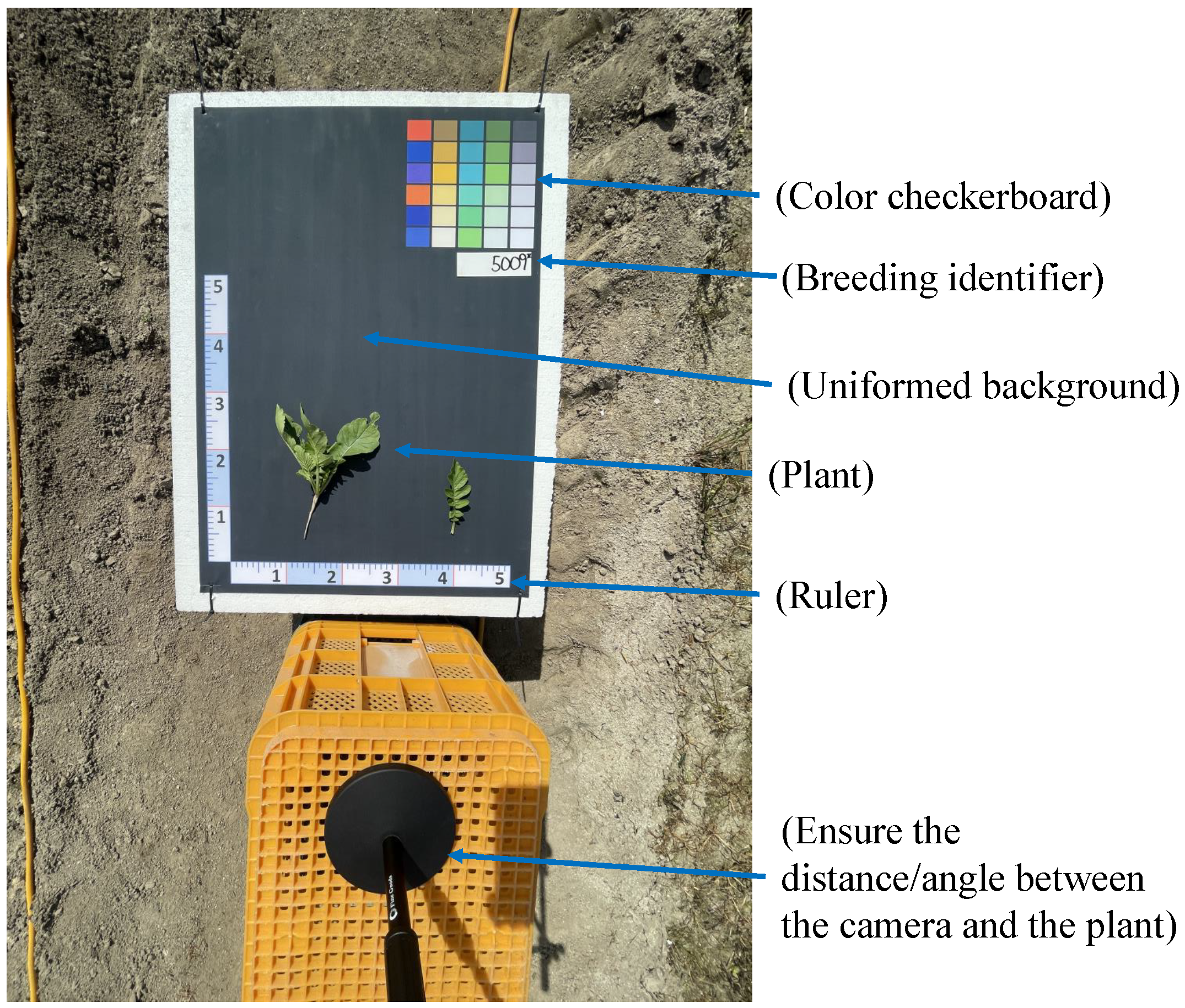
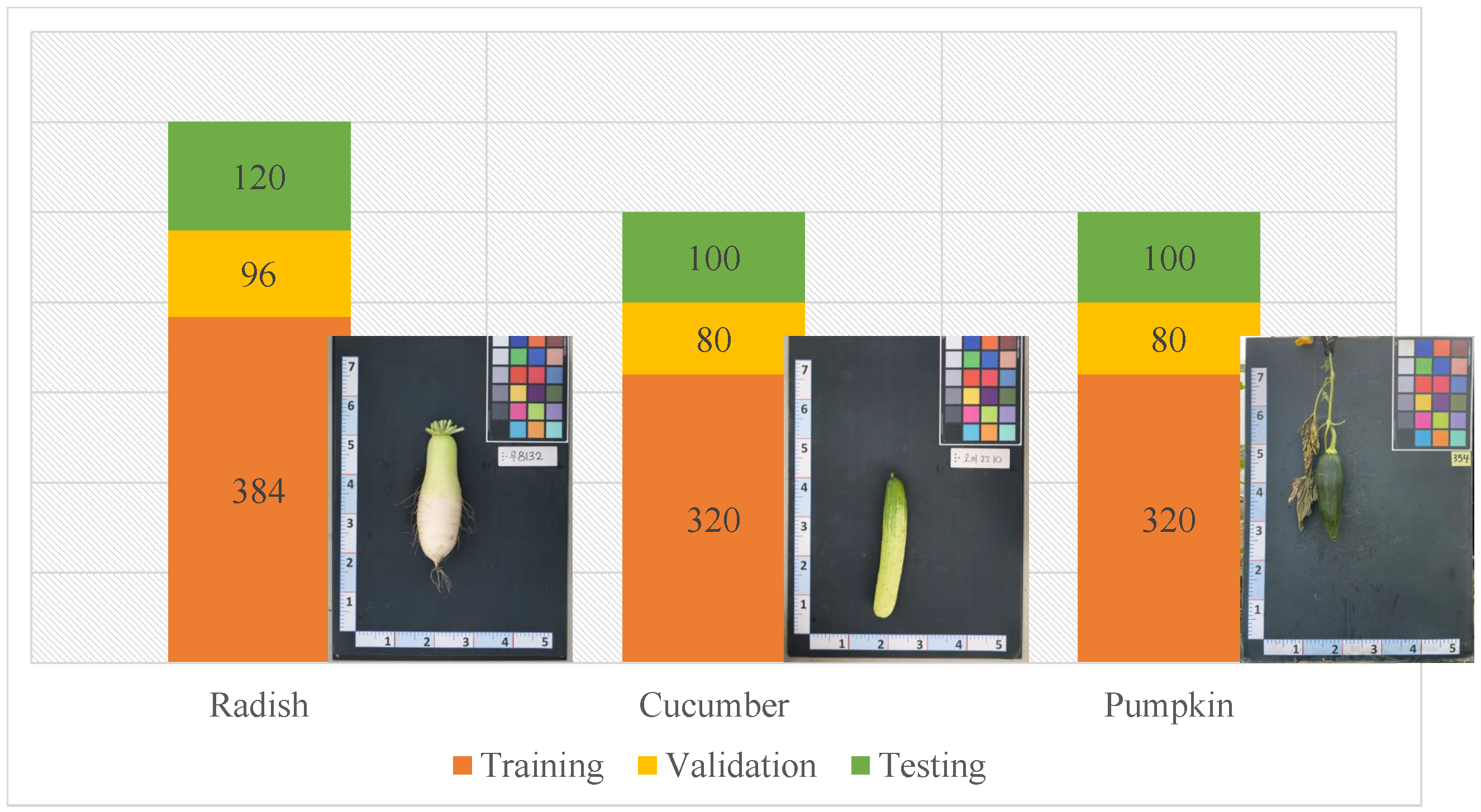
2. Plant Phenotypic Dataset

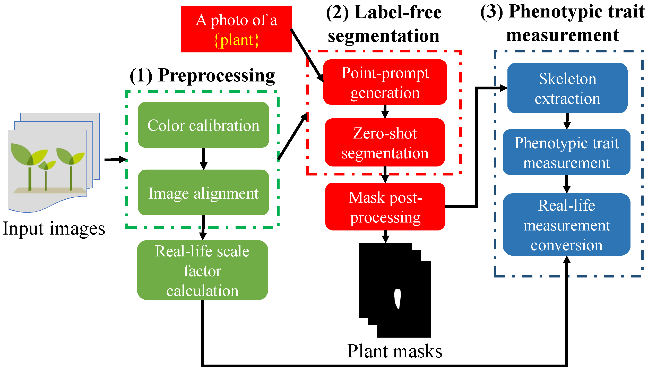
To validate the effectiveness of the zero-shot plant recognition approach against supervised methods, this study introduces a sample phenotype database. This dataset comprises images of three plant varieties: radish, cucumber, and pumpkin. These images were taken using a Samsung Galaxy S22 ultra. This smartphone was chosen over a digital camera for several reasons. Firstly, the phone comes equipped with a high spatial resolution 50-megapixel rear camera, an f/1.8 aperture, and precise autofocus capabilities, which are more than sufficient for capturing high-resolution images (https://www.gsmarena.com/samsung_galaxy_s22_5g-11253.php, accessed on 7 January 2024). Secondly, the use of a smartphone allows greater flexibility and portability, as it is easier to handle and maneuver in various environments compared to a digital camera. Lastly, the widespread availability and usage of smartphones make them a more accessible tool for similar studies in the future, potentially promoting larger-scale data collection and collaboration.

The data collection was conducted in a controlled greenhouse facility in Kyonggi-do, Korea, from August 2022 to June 2023. A constant temperature of 22${ }^{\circ }$C ± 2${ }^{\circ }$C and a stable humidity of 70% ± 5% were maintained in the greenhouse. Plants were drip-irrigated three times daily with a nutrient solution enriched with potassium, phosphorus, nitrogen, and other essential elements to minimize abiotic stresses like nutrient deficiencies and drought. Daily inspections by experienced farmers/experts prevented disease and pest outbreaks, resulting in less than 5% of plants affected throughout the experiment.

To maintain uniform lighting conditions and reduce variations between collected images, the data collection was carried out within a ninety-minute window around solar noon (11:00 a.m.–12:30 p.m.). Additionally, periods of partial cloud cover were actively avoided during this time. For accurate color representation and cross-dataset calibration, an X-Rite ColorChecker Classic (https://www.xrite.com/categories/calibration-profiling/colorchecker-classic, accessed on 7 January 2024) was attached to the imaging platform, allowing for consistent calibration and color representation throughout the dataset.

Figure 1 demonstrates the standardized procedure adopted for capturing images with a smartphone. A tripod was employed to fix the smartphone camera at a uniform distance and angle relative to the imaging platform. The tripod was placed at the bottom side of the platform. A standing stick served as a constant reference for maintaining the correct positioning throughout the image acquisition process. This setup ensured that each image was taken with consistent alignment, thus reducing variations and increasing the reliability of the subsequent processes.

Figure 2 shows the distribution of 1600 annotated plant images across training, validation, and testing sets. We allocated 80% of the data, equivalent to 1280 images, for training and validation. Out of these, 1024 images were used for training and the remaining 256 images for validation. The rest of the dataset, comprising 20% or 320 images, was reserved for testing.

3. System Overview

The main phases of the zero-shot plant component recognition and phenotypic trait measurement framework are outlined in Figure 3.

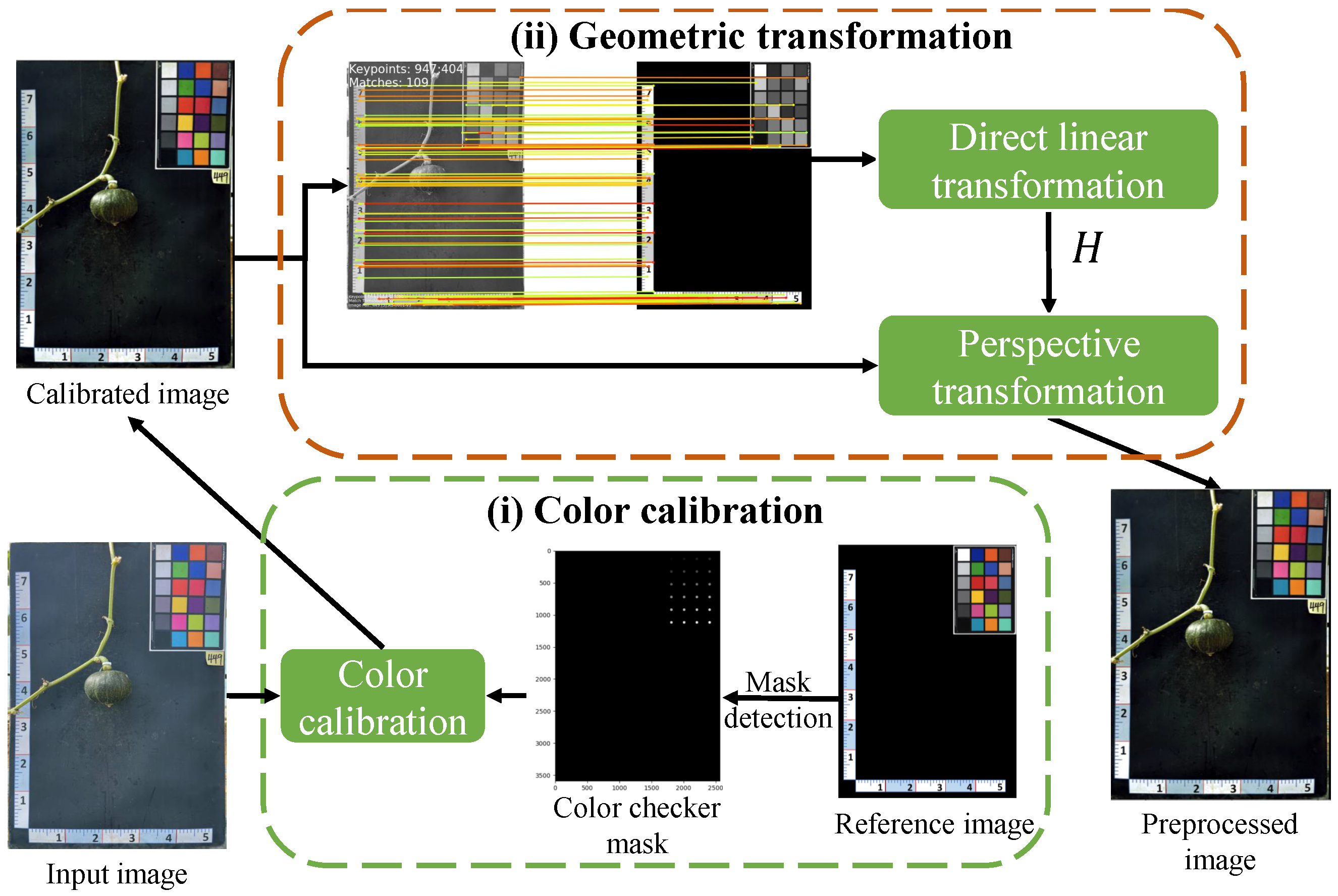
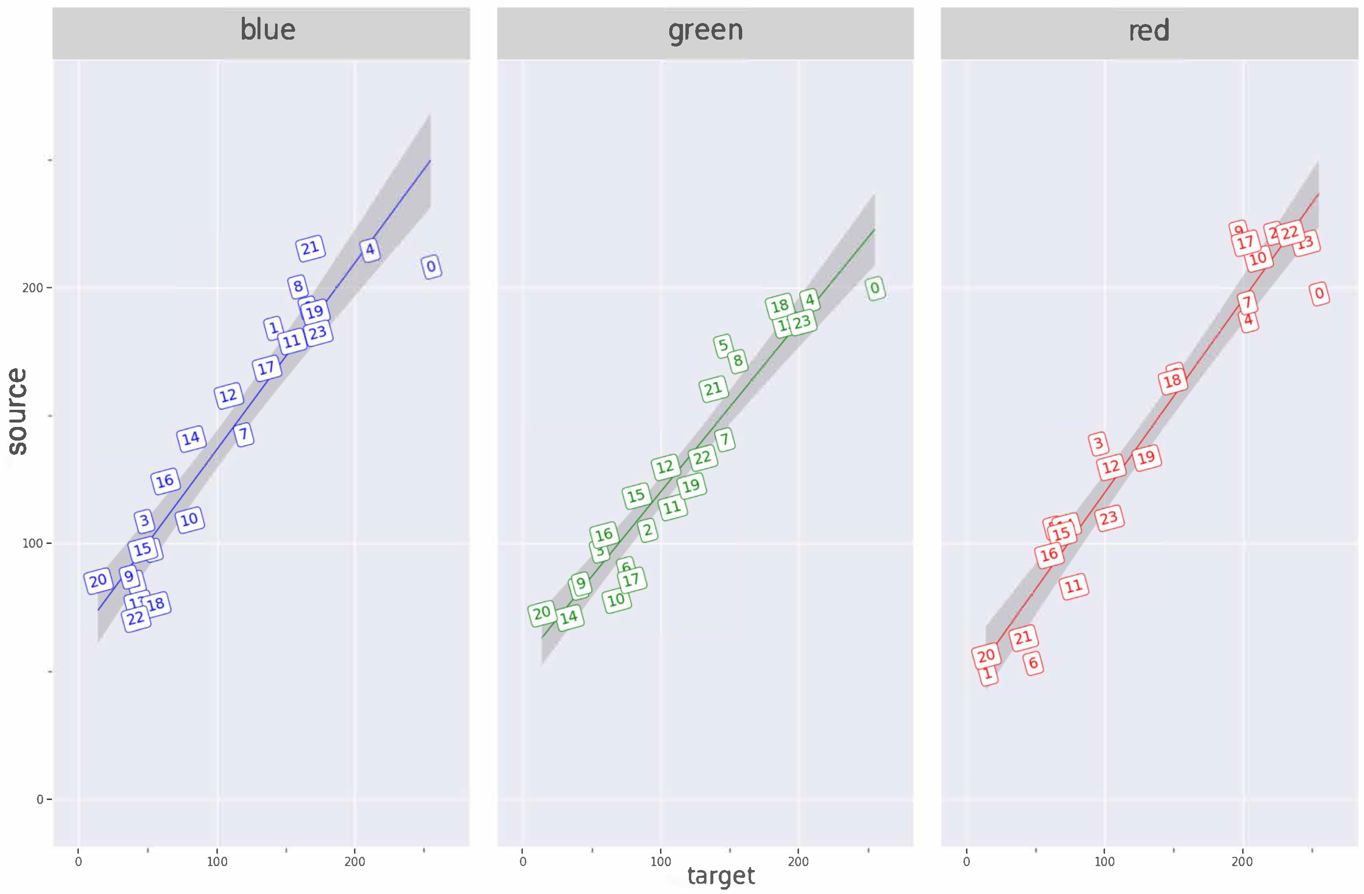
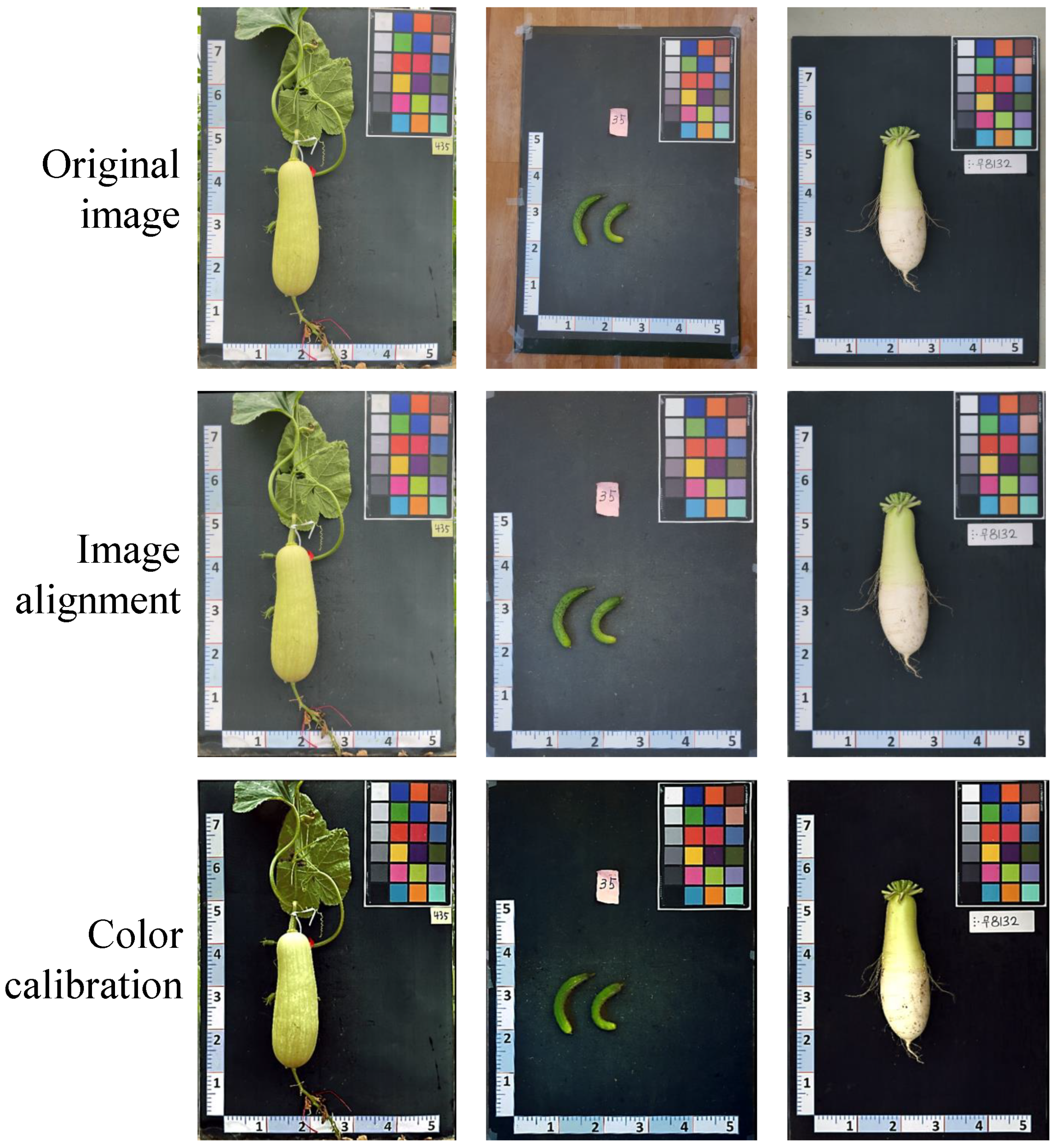
• Preprocessing: Preprocessing plays a crucial role in ensuring accurate plant trait identification. In this study, two preprocessing methods, namely, color calibration and image alignment, were carried out. Color calibration corrects inconsistencies in color reproduction caused by camera settings, lighting variations, or sensor specifications. On the other hand, image alignment addresses misalignment arising from camera movement, wind-blown plants, or uneven terrain. After the preprocessing step, a scale factor is calculated to facilitate the conversion of measurements from an image space system into an object space system.
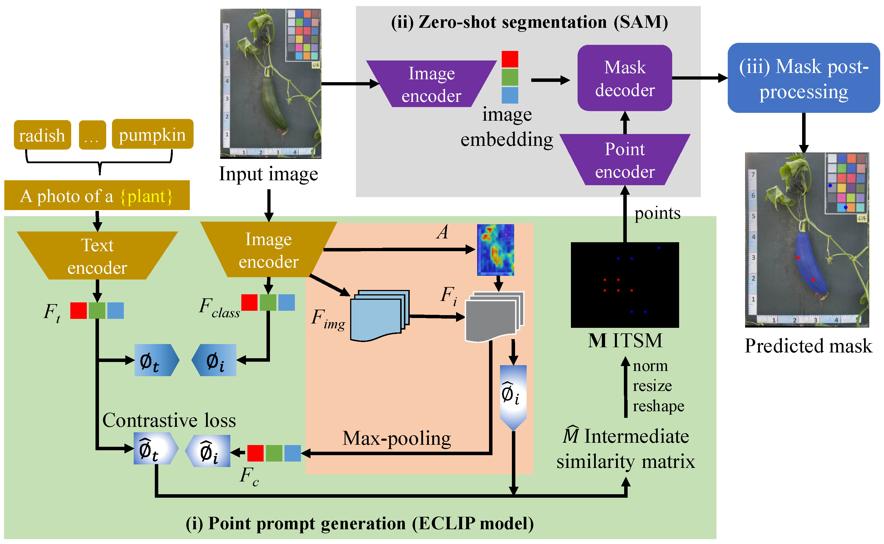
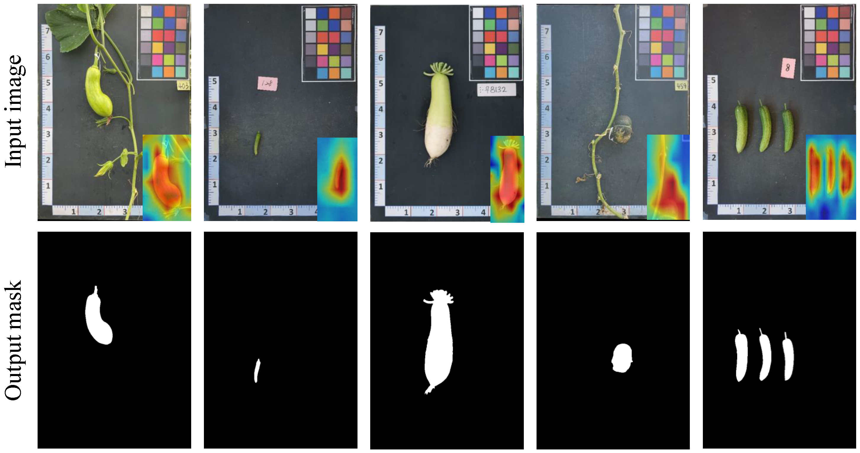
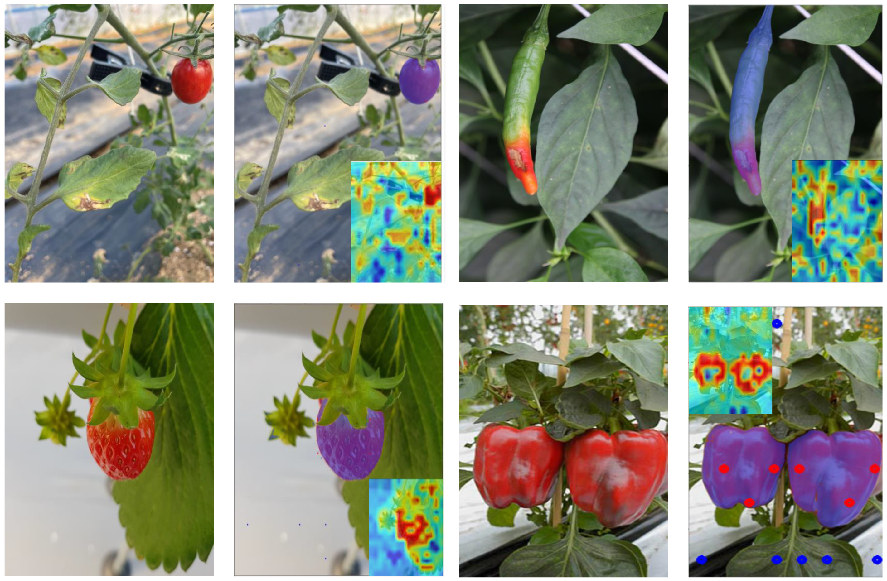
• Label-free segmentation: The zero-shot segmentation method bypasses the requirement for conventionally labeled datasets by utilizing the capabilities of pretrained large models. ECLIP, a pretrained image-text model, processes textual descriptions of plant parts and directly generates keypoint locations on the image. These points serve as guiding signals for SAM, a powerful segmentation model, allowing it to identify and segment the plant components. Finally, a postprocessing step refines the segmentation mask, eliminating wrongly segmented regions and ensuring a clean, accurate representation of the plant for further analysis.
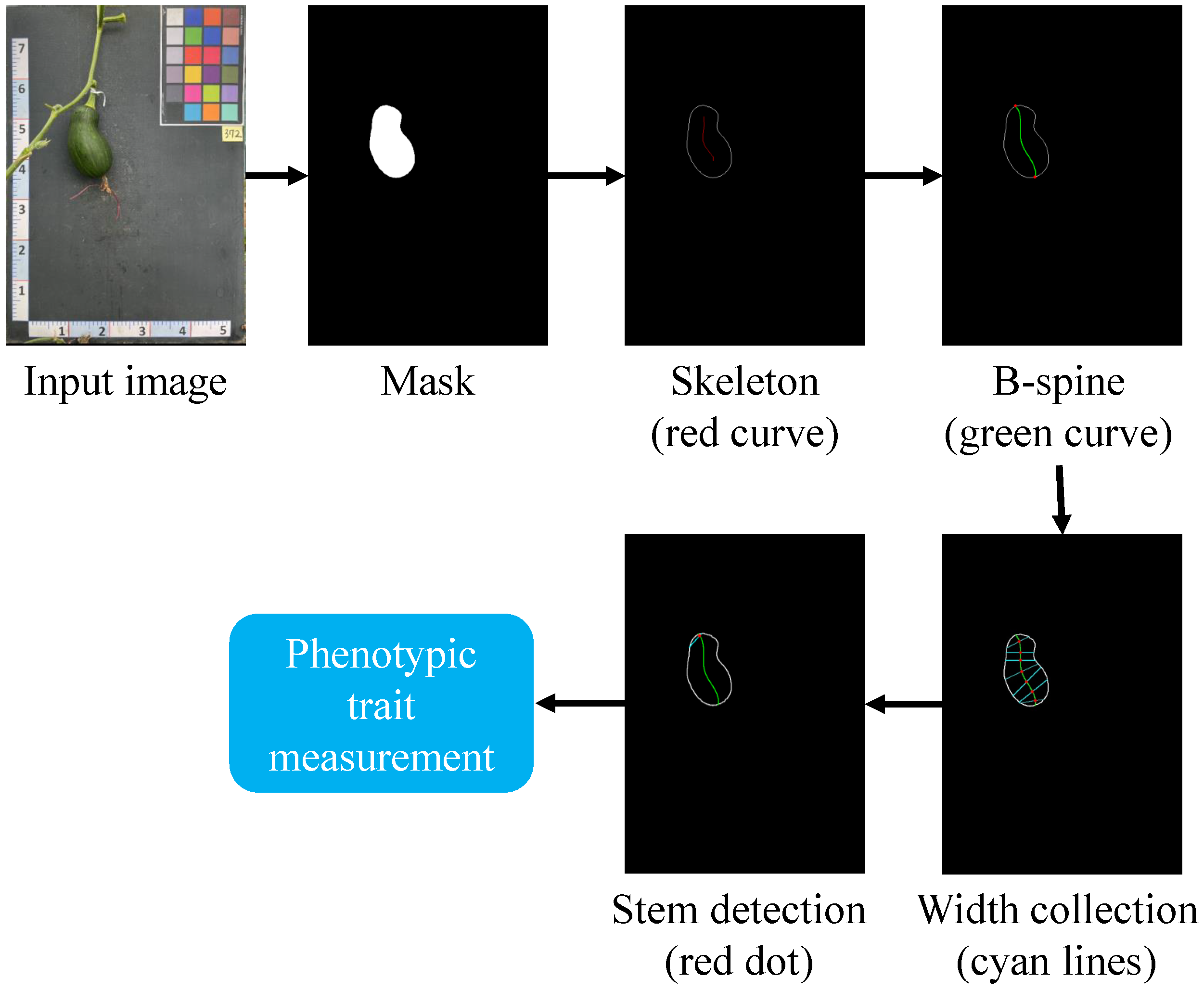
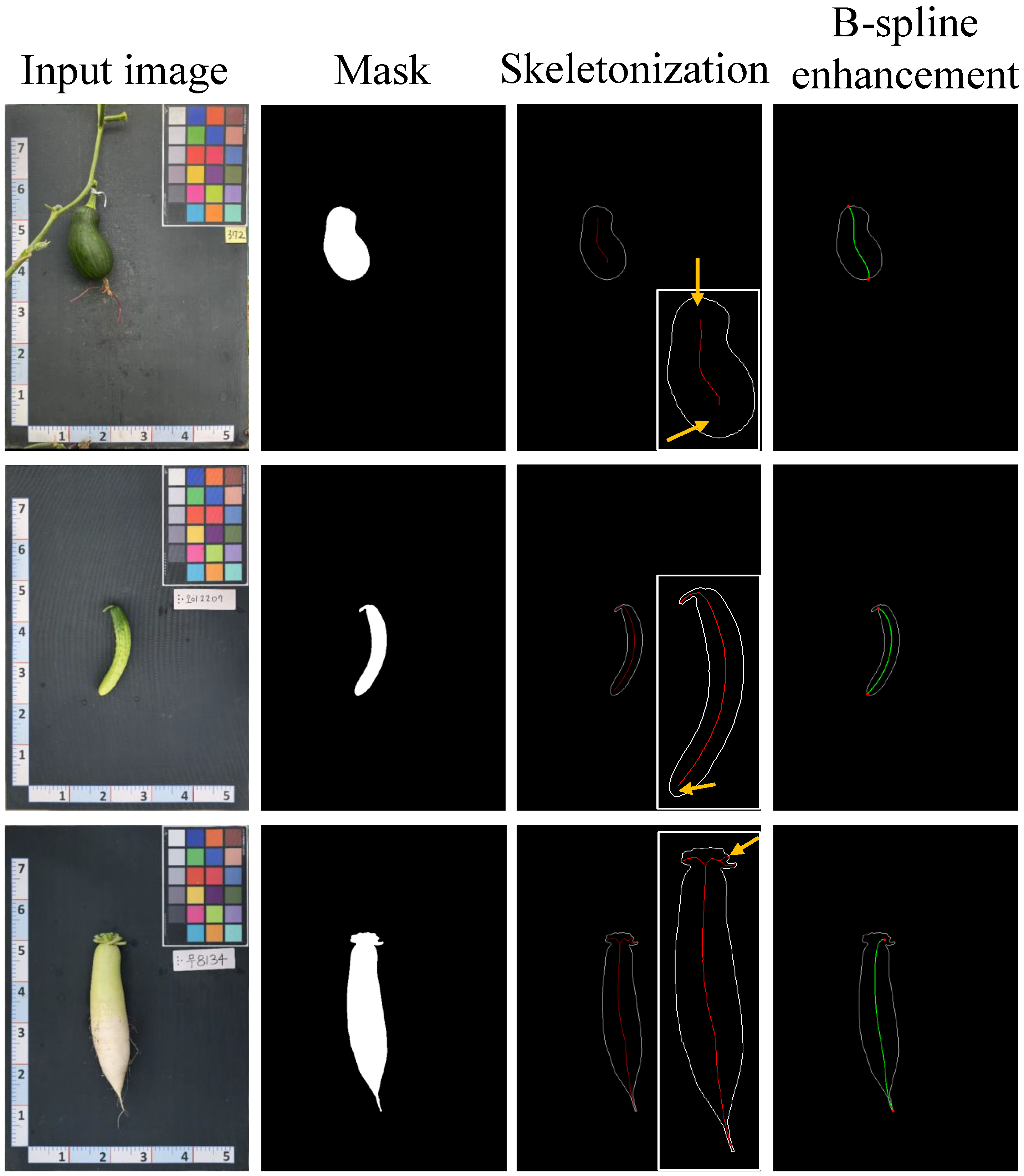
• Phenotypic trait measurement: By utilizing the segmented masks created by the label-free segmentation module and the calculated scale factor (converting the image space system into the object space system), we can accurately measure various plant phenotypic traits, such as width and length, in real-world units.

4. Methodology

4.1. Preprocessing

Given that the dataset was collected under real-world conditions, it could be affected by various factors leading to inconsistencies in the images. To ensure the quality of the dataset, we performed color calibration. After that, an additional geometric transformation module was implemented. This module realigns all the captured images to a standardized angle and distance to ensure accurate phenotypic trait measurement across different images. Figure 4 explains the main processes in each preprocessing method, including (i) color calibration and (ii) geometric transformation.

4.1.1. Color Calibration

Color calibration is crucial for ensuring consistent and accurate colors in images captured under varying lighting conditions. In this process, a reference chart with known color values, is attached to an imaging platform during image capture [19]. The captured images are then processed, and the colors are adjusted to match the color values of the checker under the same lighting conditions. This method ensures that the images reflect the actual colors of the subjects, regardless of changes in lighting or camera settings. This is particularly important in studies like ours, where accurate color representation can significantly affect the accuracy of extracting phenotypic traits [20].

Under ideal circumstances, there should be a direct linear relationship between the corresponding RGB values of color patches in the target image (controlled conditions) and source image (outdoor conditions). However, target images are prone to variable lighting conditions, which can cause deviations from the presumed linear relationship. Figure 5 compares color check matrices from the source and reference images. These matrices show the average red, green, and blue (R, G, and B) values for each color patch in both images. It is evident that across all color channels, some patches in the source image deviate from the expected linear trend line. This deviation highlights the crucial role of color calibration for precise and reliable results.

4.1.2. Image Alignment

Within the framework of the pinhole camera model, a homography matrix, denoted as H, establishes a fundamental link between two images of the same scene captured from distinct viewpoints, assuming that camera motion preserves scene geometry [21]. H takes the form of a $3\times 3$ matrix with 8 degrees of freedom (DoF) and represents a planar projective transformation capable of mapping points from a source image to their corresponding counterparts in a target template (captured from a different viewpoint) [22].

In this study, we used a flat-surface imaging platform. To align the input images with the perspective of the imaging platform template, we applied a technique called homography transformation, also known as perspective transformation [23]. Homography matrix estimation has long been a well-established task in CV.

Recently, Sarlin et al. [24] unveiled SuperGlue, a graph neural network trained on top of SuperPoint keypoints and descriptors, facilitating robust feature matching. SuperGlue excels at modeling relationships between various elements within a graph structure. The graph nodes represent individual keypoints detected in images, while the edges symbolize potential matches between these keypoints. We chose SuperGlue for homography estimation due to the availability of its pretrained model, which exhibits real-time performance across diverse settings.

Figure 4(ii) illustrates the main steps in the image alignment module. This module begins by pairing an input image containing a plant sample with an imaging platform reference template. The pretrained SuperGlue model is utilized to accurately identify matching point pairs across the two images. These matched pairs serve as the foundation for calculating the homography matrix H, which encapsulates the relationship between the two perspectives. Finally, the perspective transformation with H serving as a crucial parameter is carried out to warp the input image.

4.2. Label-Free Segmentation

Recent advancements in zero-shot vision models, like ECLIP [18] and SAM [17], have enabled the direct application of powerful pretrained DL models for plant recognition. This development obviates the need for data annotation and model training for specific plants. As illustrated in Figure 6, we employ these models to achieve precise segmentation of key plant components (e.g., leaves, fruits) without time-consuming manual labeling. However, the resulting plant masks can contain multiple overlapping masks and background noise. To address this, a postprocessing phase is implemented to eliminate excessively small or large masks, and highly overlapping ones are merged based on predefined threshold parameters (Section 4.2.3).

4.2.1. Point Prompt Generation

Contrastive Language–Image Pretraining (CLIP) [25] is an ML approach that learns to understand and generate meaningful representations of images and text in a shared embedding space. In CLIP, contrastive learning is employed to train the model. This technique involves presenting the model with pairs of images and text, where the task is to determine whether each pair represents a matching image–text combination or not. All these pairs are drawn from the same dataset. This allows it to learn diverse visual concepts described in natural language and apply this understanding to both images and text. As a result, CLIP can perform various tasks like zero-shot classification and object detection without needing task-specific training data. Despite improving the performance of numerous CV tasks, the visual explainability of these models, including in their raw feature maps, has been rarely studied.

ECLIP, an enhanced version of the CLIP model by Li et al. [18], allows visual explanations of its predictions through an Image–Text Similarity Map (ITSM). This map measures the similarity between each image’s feature map and the embedding of its corresponding text description. An ITSM can be employed to recognize image regions most relevant to the text description. Li et al. also discovered a semantic shift issue, where CLIP prioritizes background regions over foregrounds, leading to visualization that contradicts human perception. To address this limitation, the original attention pooling is replaced with max pooling guided by free attention during training. This prioritizes informative foreground features, resulting in visualizations that align better with human understanding.

Given a self-supervised image encoder $f_i$ and text encoder $f_t$ along with their corresponding linear projections ${\varphi }_i$ and ${\varphi }_t$ (a function that learns a 2D parameter matrix), the image features $F_i\in {\mathbb{R}}^{N_i\times C}$ and text features $F_t\in {\mathbb{R}}^{N_t\times C}$ from image input $x_i$ and text input $x_t$ can be extracted as follows:

$$\left\{F_c,F_i\right\}=f_i\left(x_i\right),F_t=f_t\left(x_t\right)$$

(1)

The feature $F_c\in {\mathbb{R}}^{1\times C}$ serves as the class token used for classification purposes. The remaining image tokens, denoted as $F_i\in {\mathbb{R}}^{N_i\times C}$, are the raw feature map. In this context, $N_i$ and $N_t$ represent the number of image tokens and text tokens, respectively, and $\mathrm{C}$ denotes the dimensionality of the embeddings. Subsequently, the intermediate similarity matrix $\widehat{M}\in {\mathbb{R}}^{N_i\times N_t}$ is computed as follows:

$$\widehat{M}=\left(\frac{F_i·{\varphi }_i}{{∥F_i·{\varphi }_i∥}_2}\right)·{\left(\frac{F_t·{\varphi }_i}{{∥F_t·{\varphi }_i∥}_2}\right)}^{\top }$$

The ITSM feature map $M\in {\mathbb{R}}^{H,W,N_t}$ is then reconstructed by reshaping and resizing using bicubic interpolation to match the input image’s dimensions (width W and height H). Additionally, min-max normalization, denoted as $Norm$ is applied to the H and W dimensions to improve visual interpretability. The resulting ITSM can be expressed as follows:

$$M=Norm(Resize(Reshape\left(\widehat{M}\right)))$$

(2)

In the context of label-free plant segmentation, foreground points from ECLIP with similarity scores exceeding 0.8 are used as point prompt input to guide SAM [18]. Concurrently, an equal number of points with the lowest ranks are designated as background points. This approach helps to avoid the poor performance experienced with SAM when solely reliant on text prompts [26].

4.2.2. Zero-Shot Segmentation

SAM is a novel artificial intelligence (AI) model from Meta AI that introduces a novel paradigm for image segmentation [18]. Unlike traditional models that need specific training for each object, SAM can handle objects it has never seen before using only prompts. This makes it adaptable for a range of segmentation tasks. The core lies in a joint embedding space, where both text and image representations are learned through contrastive learning techniques. This shared space facilitates seamless alignment between user prompts and visual features, enabling SAM to interpret nuanced textual instructions and reflect them accurately in the segmented output. SAM was trained on 11 million images and 1.1 billion segmentation masks, making it the largest dataset for segmentation to date.

As depicted in Figure 6(ii), the architecture of SAM is made up of three main modules: an image encoder, a prompt encoder, and a mask decoder. The image encoder is responsible for processing the input image and extracting essential visual features that can be applied universally across various object classes in zero-shot segmentation. It employs Vision Transformers (ViTs) to divide the image into patches and extract features from each patch, capturing both specific object details and background information. The prompt encoder can accommodate two types of prompts: sparse (points, boxes, and texts) and dense (masks).

Given the unknown location of the plant in the input image, we use the point prompt proposed by the ECLIP model (Section 4.2.1) as input to the prompt encoder. This encoder then transforms the point prompt into a latent representation. Finally, the output from the prompt encoder is concatenated with the output from the image encoder. This combined output is then fed into the mask decoder, which predicts a segmentation mask for the input image.

4.2.3. Mask Postprocessing

When using points as input prompts for segmentation, the resulting segmented masks often contain many highly overlapping masks and noise blobs from the background. To tackle this issue, we implemented a mask postprocessing algorithm. The algorithm removes excessively large or small masks and merges masks that are duplicated or substantially overlapped based on two thresholds: intersection over union (IoU) and overlap ratio. Masks exceeding predefined thresholds for IoU or overlap ratio are merged into a single mask.

• Initialize an empty list $selected\_masks$ to store the masks that meet the area criteria.
• For each mask in the output masks from SAM:

  −

  Find the largest contour in the mask and calculate its area.

  −

  If the area of the largest contour is within the range of $min\_area$ and $max\_area$, add the mask to $selected\_masks$.

• Initialize an empty list $final\_results$ to store the final selected masks.
• While $selected\_masks$ is not empty:

  −

  Remove one mask from $selected\_masks$ and assign it to $pivot\_mask$.

  −

  For each remaining mask in $selected\_masks$:

  ∗

  Calculate the IoU and the overlap ratio between the $pivot\_mask$ and the current mask.

  ∗

  If the IoU is greater than a threshold $iou\_threshold$ or the overlap ratio is greater than a threshold $overlap\_threshold$, merge the current mask with the $pivot\_mask$.

  −

  Add the $pivot\_mask$ to $final\_results$.

Given the varying sizes of the three plant types in our dataset, only masks with the area that fall within the range of 5% to 50% of the total image area were reserved. This decision was based on the inherent characteristics of the plant sizes. When it came to merging duplicate masks, an overlap threshold and an IoU threshold at 0.88 were established. This value was chosen in line with the default threshold set for SAM [17].

4.3. Phenotypic Trait Measurement

The segmented plant masks extracted from the label-free segmentation module can be used to precisely measure the phenotypic traits, such as width and length. The length is defined as the longest segment of the central line through the organ, excluding the stem. However, it is challenging to determine the width of a plant because there are countless lines that can be drawn perpendicular to the plant’s central axis. As a result, the measured width can vary depending on the specific line chosen for measurement.

Therefore, the width trait was measured at various points along the medial axis to create a collection of width measurements represented as $w=(w_1,\dots ,w_n)$. If a single width value is required, the median of the width profile can be computed as $\tilde{w}=med\left(w\right)$. The measurement pipeline is illustrated in Figure 7.

To capture the general structure of the input mask, skeletonization was first applied to obtain a coarse representation of its medial axis. However, the resulting coarse medial axis may have multiple branches and may not intersect with the mask’s boundary due to the complex shape of some plants. To address these issues and improve measurement accuracy, a basic spline (B-spline) curve [27] is fitted to the coarse medial axis of the skeleton. A B-spline is a polynomial function defined piece-wise that is widely utilized across various fields to represent curves and surfaces. A B-spline curve, denoted as $P\left(t\right)$, is defined as follows:

$$P\left(t\right)=\sum _{i=0}^n{Q}_i{N}_{i,d}\left(t\right)$$

(3)

where $N_{i,d}$ are the B-spline basis function of degree j and ${\left\{Q_i\right\}}_{i=0}^n$ are the control points. The basis function of a B-spline are defined recursively and depend on the knot vector, which is a non-decreasing sequence of real numbers. The knot vector is denoted as $T=\left\{t_0,t_1,\dots ,t_m\right\}$, where T is a non-decreasing sequence and each $t_i$ is within the interval $[0,1]$. The control points are defined as $P_0,\dots ,P_n$. The degree is given by $p=m-n-1$. The “knots” $t_{p+1},\dots ,t_{m-p-1}$ are referred to as internal knots.

$$N_{i,0}\left(t\right)=\left\{\begin{array}{cc}1,\hfill & \mathrm{if}{t}_i\le t\le t_{i+1}\mathrm{and}{t}_i\le t_i\le t_{i+1}\hfill \\ 0,\hfill & \mathrm{otherwise}\hfill \end{array}\right.$$

(4)

For $j=1,2,\dots ,p$, the basis function is defined by the recursion:

$$N_{i,j}=\frac{t-t_i}{t_{i+j}-t_i}{N}_{i,j-1}\left(t\right)+\frac{t_{i+j+1}-t}{t_{i+j+1}-t_{i+1}}{N}_{i+1,j-1}\left(t\right)$$

(5)

4.3.1. Implementation Descriptions

The framework for label-free plant recognition and phenotypic trait measurement was built using PyTorch, a popular machine learning library for Python. This system was run on a Linux system, equipped with two Nvidia Tesla V100 graphics processing units, each with 32 gigabytes of memory. We implemented all DL models and hyper-parameters, with the exception of the zero-shot segmentation model, using open-source code from the original papers. To ensure reliable experiments, a pretrained Vision Transformer (ViT) model on ImageNet was utilized as the backbone for all segmentation models.

4.3.2. Evaluation Metrics

In this research, the primary metric used to evaluate the performance of the segmentation model is the IoU. This metric calculates the ratio of the number of pixels shared between the target and prediction masks to the total number of pixels in both masks. The formula for IoU is given below:

$$IoU=\frac{TP}{TP+FP+FN}$$

(6)

The model’s accuracy in predicting phenotypic traits is evaluated using the Mean Absolute Error (MAE). The MAE is a statistical measure that quantifies the average magnitude of errors between paired predicted and actual values. A lower MAE indicates that the model’s predictions are generally closer to the true values, which signifies better performance.

$$MAE=\frac{1}{n}\sum _{t=1}^n\left|A_i-{\widehat{A}}_i\right|$$

(7)

where n denotes the total number of fitted points. $A_i$ indicates the actual value, while ${\widehat{A}}_i$ represents the predicted value. The absolute value operator $|.|$ guarantees that all errors are expressed as positive values, making it easier to compare the discrepancies.

5. Experimental Results

5.1. Preprocessing

Figure 8 demonstrates the crucial role of preprocessing, including image alignment and color calibration, on three different plant species: pumpkin, cucumber, and radish. Notably, the image alignment module effectively realigns the input images to a precise bird’s-eye view of the imaging platform, discarding irrelevant regions and simplifying downstream processing tasks. Subsequently, the realigned images are fed into the color calibration, which leverages a reference template to rectify inconsistencies in color reproduction.

The resulting output images exhibit remarkably improved visual fidelity, matching more closely with their real-life counterparts. The results underscore the importance of preprocessing in enabling accurate and reliable segmentation and phenotypic trait measurement outcomes.

5.2. Zero-Shot Plant Component Segmentation Performance Analysis

Table 1. Performance of the proposed zero-shot segmentation for the three plant types on the testing set.

Metrics	Pumpkin	Radish	Cucumber
mIoU	70.2	73.7	68.4
Precision	69.1	72.1	70.2
Recall	71.5	70.8	70.7

presents the performance of the proposed zero-shot plant component recognition model for each of the three plant types in the dataset, which include radish, cucumber, and pumpkin. The table reports the IoU, precision, and recall scores.

Despite the challenges of real-world data (e.g., varying lighting and occlusions), our zero-shot plant component segmentation framework achieves good performance (average IoU: 70.7%) on all three plant types. This suggests that our model can effectively segment various plant components without any specific training data for those types. Radish achieves the highest IoU (73.7%), followed by pumpkin (70.2%) and cucumber (68.4%).

This indicates that the model might struggle slightly with certain aspects of cucumber segmentation compared to the other two plant types. One possible explanation for the relatively low segmentation performance of cucumbers is that they are relatively small compared to the background. Additionally, up to 5 cucumbers may be placed together in the same image, which further complicates the segmentation process.

Figure 9 shows two key representations for each of the three plant types: (1) the original image and ECLIP attention masks highlighting relevant plant parts and (2) the final predicted masks after applying the postprocessing process. Across all plant varieties, the ECLIP exhibits remarkable accuracy in detecting relevant plant components within the images through the attention masks. Finally, guided by ECLIP, SAM accurately predicts plant masks, closely adhering to the boundaries of plant components. The zero-shot segmentation approach also works well in challenging cases, such as when a pumpkin is partially obscured by a leaf or when numerous tiny cucumbers appear in an image. The model effectively identifies all of them.

Figure 10 demonstrates the predicted masks from the proposed zero-shot model for four novel plants in real-world settings without specific backgrounds and controlled lighting conditions. The first column shows the original images, while the second column displays the attention masks generated by iCLIP, highlighting potentially significant components. Additionally, the figure overlays the predicted plant masks on the original images. Overall, iCLIP’s attention masks effectively pinpoint potentially important plant component areas in the image, even for plants with various shapes and backgrounds. Therefore, the attention masks accurately guide SAM to generate precise segmentation of plant components.

Table 2. Performance of the zero-shot approach compared to two supervised models on the testing dataset.

Model	mIoU	Precision	Recall
SOLOv2 [28]	73.9	74.6	74.2
Mask-RCNN [13]	75.3	74.8	75.1
Ours (ECLIP+SAM)	70.7	70.4	71

presents a comparative analysis of the proposed zero-shot segmentation approach with two supervised methods, namely, Segmenting Objects by Locations (SOLOv2) [28] and Mask-RCNN [13], on the testing dataset.

In the evaluation of various models, Mask-RCNN emerged as the top performer, achieving the highest mIoU (75.3%), precision (74.8%), and recall (75.1%). DeepLabv3 demonstrated mIoU scores comparable to SOLOv2 at 73.9%. While the proposed zero-shot approach obtained a slightly lower mIoU (70.7%) compared to the two supervised models, its implementation does not require a time-consuming training process. Moreover, this zero-shot method can be easily used with new types of plants. This is a major benefit in situations where there is little or no annotated training data available.

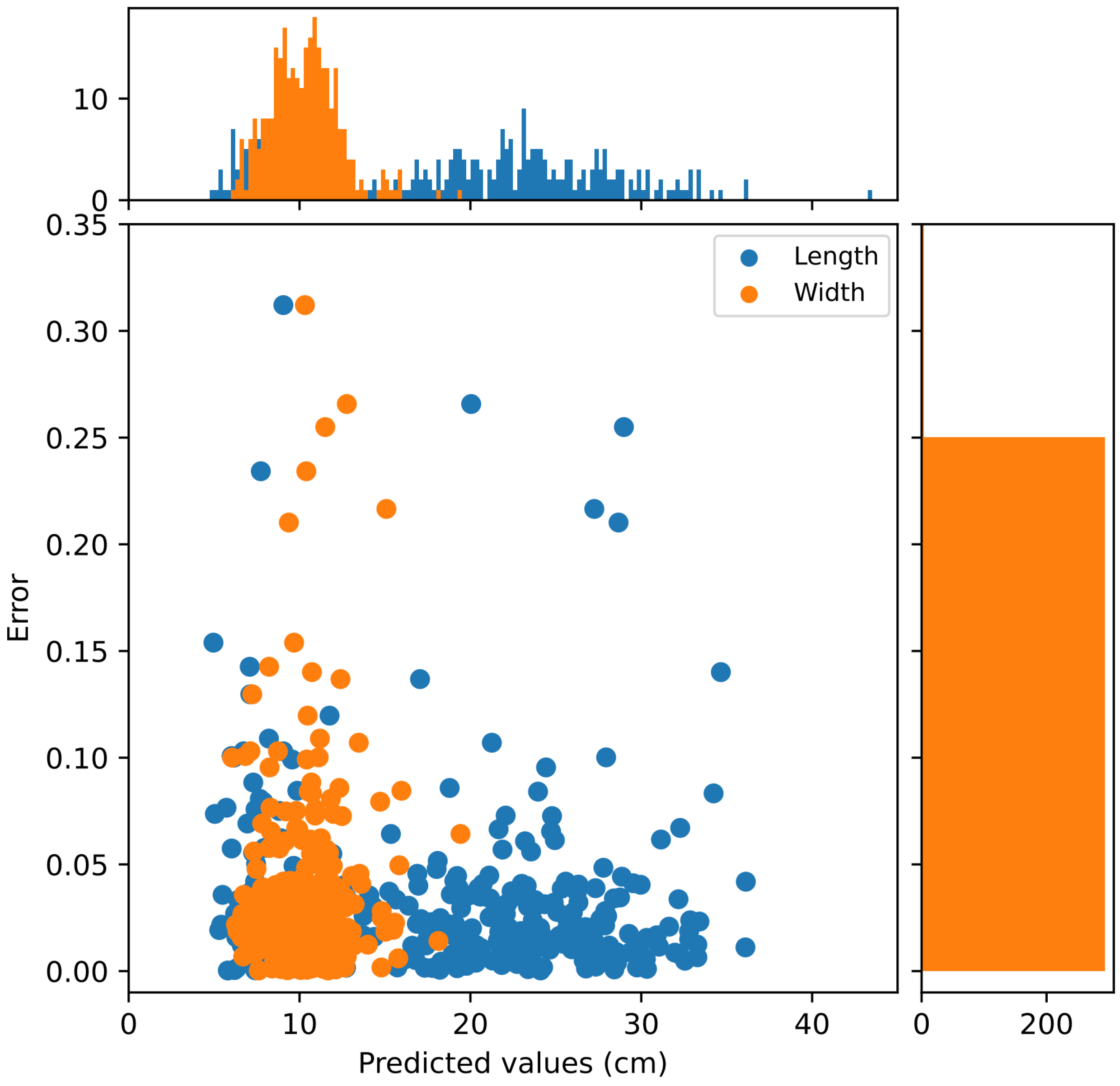
5.3. Phenotypic Trait Measurement

Figure 11 visualizes the skeletonization process within the context of phenotypic trait measurement. After obtaining the output masks from the zero-shot plant recognition model, the subsequent steps involve skeletonization and B-spline curve enhancement.

The skeletonization algorithm simplifies and emphasizes the geometrical and topological properties of the plant shape, such as length, direction, and branching. This process is crucial for estimating phenotypic traits accurately. However, as we can observe, the skeletons extracted from the skeletonization process often fail to fully capture the object boundaries. This is particularly the case for the pumpkin and cucumber samples, as highlighted by the arrows. Furthermore, these skeletons exhibit noise, which leads to multi-branched and non-smooth structures. This is evident in the radish sample.

By integrating the B-spline curve into the skeletonization process, we can overcome the limitations associated with using the skeletonization process alone. The resulting skeletons offer a precise and effective solution. The enhancement of the B-spline curve further refines the representation of the plant component structure. Figure 11 also highlights the precision of our suggested approach in identifying the stem region of the three plants.

To assess the accuracy of our phenotypic trait measurements, we randomly selected 300 samples from the testing dataset. For each of these samples, we manually recorded the ground truth values of width and length traits using the ruler included in each image. After that, we converted the predicted length and width trait measurements for each test image from the 2D image space system into the real-world object space system using the scale factor. The scale factor $0.1048$ was calculated based on the ruler on the standard reference image (Figure 3).

Figure 12 provides an analysis of measurement performance by plotting the error distributions against the predicted width and length. In most cases, the MAE stays within $0.05$. However, some outliers exhibit MAE errors exceeding $0.1$ for both length and width, which is alarmingly high. Upon investigating the failure cases, we found that the most common source of error lies in accurately detecting the stem part. Accurate identification poses a significant challenge in the case of immature samples, where the width of the stem deceptively mirrors that of the body part.

6. Conclusions and Future Works

This research presents a simple and efficient framework for zero-shot plant identification and the automated measurement of key plant phenotypic traits, particularly length and width. Our framework utilizes recent advancements in DL approaches, specifically pretrained segmentation models capable of performing precise segmentation without the requirement for an annotated dataset or model training, setting it apart from traditional approaches. Our research presents a significant advancement in plant phenotyping methodologies, offering a scalable and adaptable solution for automated plant trait measurement. The insights gained from this study can be applied to other plant phenotyping methodologies, contributing to the broader goal of accelerating the development of resilient and productive crops.

Firstly, we propose an image alignment correction module that aligns the input images to ensure a consistent orientation to a specific template (e.g., a correct image alignment template). This cost-effective approach avoids the need for a complex imaging platform and can be easily adapted to various template types. After that, a zero-shot plant recognition model based on SAM and ECLIP is introduced. It performs well for objects that have a consistent color and texture and are clearly distinguishable from the background, such as plants with uniform coloration and well-defined boundaries compared to the surrounding background. In addition, a mask postprocessing step is introduced to refine the predicted masks by the zero-shot segmentation approach by removing noise and duplicate masks.

Finally, a B-spline curve is implemented during the skeletonization process to improve robustness against noise from segmentation outcomes and enhance the reliability of length measurements, which was proved to achieve more precise plant skeletons compared to the direct use of morphological skeletons. The experimental results from 300 samples showed that the proposed system achieved a precise measurement, as evidenced by an MAE of around 0.06 for most samples. Moreover, an MAE of less than 0.05% error rate was observed in 85.75% of the samples, underscoring the robustness of our methodology. This valuable insight can be applied to other plant phenotyping methodologies that rely on morphological skeletons for medial axis extraction.

While this study focused on measuring the phenotypic traits of three specific plants (pumpkin, radish, and cucumber), the framework can be easily adapted to other species with appropriate parameter adjustments. However, due to its current complexity, real-time measurement remains unsupported. In the future, our focus will be on enhancing the framework’s robustness and reducing its computational complexity to facilitate real-time processing. Additionally, there are challenges in accurately detecting the stems in some samples. The high similarity in width between the stem and the plant body introduces a challenging case that requires further investigation. It is conceivable that a supervised ML model can be implemented to comprehensively tackle this problem.

References

1. Pieruschka, R.; Schurr, U. Plant phenotyping: Past, present, and future. Plant Phenomics 2019, 2019, 7507131. [Google Scholar] [CrossRef]
2. Sade, N.; Peleg, Z. Future challenges for global food security under climate change. Plant Sci. 2020, 295, 110467. [Google Scholar] [CrossRef]
3. Reynolds, M.; Chapman, S.; Crespo-Herrera, L.; Molero, G.; Mondal, S.; Pequeno, D.N.; Pinto, F.; Pinera-Chavez, F.J.; Poland, J.; Rivera-Amado, C.; et al. Breeder friendly phenotyping. Plant Sci. 2020, 295, 110396. [Google Scholar] [CrossRef]
4. Li, Z.; Guo, R.; Li, M.; Chen, Y.; Li, G. A review of computer vision technologies for plant phenotyping. Comput. Electron. Agric. 2020, 176, 105672. [Google Scholar] [CrossRef]
5. Falster, D.; Gallagher, R.; Wenk, E.H.; Wright, I.J.; Indiarto, D.; Andrew, S.C.; Baxter, C.; Lawson, J.; Allen, S.; Fuchs, A.; et al. AusTraits, a curated plant trait database for the Australian flora. Sci. Data 2021, 8, 254. [Google Scholar] [CrossRef]
6. Dang, M.; Wang, H.; Li, Y.; Nguyen, T.H.; Tightiz, L.; Xuan-Mung, N.; Nguyen, T.N. Computer Vision for Plant Disease Recognition: A Comprehensive Review. Bot. Rev. 2024, 1–61. [Google Scholar] [CrossRef]
7. Yang, W.; Feng, H.; Zhang, X.; Zhang, J.; Doonan, J.H.; Batchelor, W.D.; Xiong, L.; Yan, J. Crop phenomics and high-throughput phenotyping: Past decades, current challenges, and future perspectives. Mol. Plant 2020, 13, 187–214. [Google Scholar] [CrossRef]
8. Li, Y.; Wang, H.; Dang, L.M.; Sadeghi-Niaraki, A.; Moon, H. Crop pest recognition in natural scenes using convolutional neural networks. Comput. Electron. Agric. 2020, 169, 105174. [Google Scholar] [CrossRef]
9. Wang, H.; Li, Y.; Dang, L.M.; Moon, H. An efficient attention module for instance segmentation network in pest monitoring. Comput. Electron. Agric. 2022, 195, 106853. [Google Scholar] [CrossRef]
10. Tausen, M.; Clausen, M.; Moeskjær, S.; Shihavuddin, A.; Dahl, A.B.; Janss, L.; Andersen, S.U. Greenotyper: Image-based plant phenotyping using distributed computing and deep learning. Front. Plant Sci. 2020, 11, 1181. [Google Scholar] [CrossRef]
11. Arya, S.; Sandhu, K.S.; Singh, J.; Kumar, S. Deep learning: As the new frontier in high-throughput plant phenotyping. Euphytica 2022, 218, 47. [Google Scholar] [CrossRef]
12. Busemeyer, L.; Mentrup, D.; Möller, K.; Wunder, E.; Alheit, K.; Hahn, V.; Maurer, H.P.; Reif, J.C.; Würschum, T.; Müller, J.; et al. BreedVision—A multi-sensor platform for non-destructive field-based phenotyping in plant breeding. Sensors 2013, 13, 2830–2847. [Google Scholar] [CrossRef]
13. Dang, L.M.; Min, K.; Nguyen, T.N.; Park, H.Y.; Lee, O.N.; Song, H.K.; Moon, H. Vision-Based White Radish Phenotypic Trait Measurement with Smartphone Imagery. Agronomy 2023, 13, 1630. [Google Scholar] [CrossRef]
14. Zhou, S.; Chai, X.; Yang, Z.; Wang, H.; Yang, C.; Sun, T. Maize-IAS: A maize image analysis software using deep learning for high-throughput plant phenotyping. Plant Methods 2021, 17, 48. [Google Scholar] [CrossRef]
15. Qiao, F.; Peng, X. Uncertainty-guided model generalization to unseen domains. In Proceedings of the IEEE/CVF Conference on Computer Vision and Pattern Recognition, Nashville, TN, USA, 19–25 June 2021; pp. 6790–6800. [Google Scholar]
16. Xian, Y.; Schiele, B.; Akata, Z. Zero-shot learning-the good, the bad and the ugly. In Proceedings of the IEEE Conference on Computer Vision and Pattern Recognition, Honolulu, HI, USA, 21–26 July 2017; pp. 4582–4591. [Google Scholar]
17. Kirillov, A.; Mintun, E.; Ravi, N.; Mao, H.; Rolland, C.; Gustafson, L.; Xiao, T.; Whitehead, S.; Berg, A.C.; Lo, W.Y.; et al. Segment anything. arXiv 2023, arXiv:2304.02643. [Google Scholar]
18. Li, Y.; Wang, H.; Duan, Y.; Xu, H.; Li, X. Exploring visual interpretability for contrastive language-image pre-training. arXiv 2022, arXiv:2209.07046. [Google Scholar]
19. Sunoj, S.; Igathinathane, C.; Saliendra, N.; Hendrickson, J.; Archer, D. Color calibration of digital images for agriculture and other applications. ISPRS J. Photogramm. Remote. Sens. 2018, 146, 221–234. [Google Scholar] [CrossRef]
20. Brunet, J.; Flick, A.J.; Bauer, A.A. Phenotypic selection on flower color and floral display size by three bee species. Front. Plant Sci. 2021, 11, 587528. [Google Scholar] [CrossRef]
21. Juarez-Salazar, R.; Zheng, J.; Diaz-Ramirez, V.H. Distorted pinhole camera modeling and calibration. Appl. Opt. 2020, 59, 11310–11318. [Google Scholar] [CrossRef]
22. Rios-Orellana, O.I.; Juarez-Salazar, R.; Diaz-Ramirez Sr, V.H. Analysis of algebraic and geometric distances for projective transformation estimation. In Optics and Photonics for Information Processing XIV; SPIE: Cergy-Pontoise, France, 2020; Volume 11509, pp. 67–81. [Google Scholar]
23. Song, L.; Wu, J.; Yang, M.; Zhang, Q.; Li, Y.; Yuan, J. Stacked homography transformations for multi-view pedestrian detection. In Proceedings of the IEEE/CVF International Conference on Computer Vision, Montreal, BC, Canada, 11–17 October 2021; pp. 6049–6057. [Google Scholar]
24. Sarlin, P.E.; DeTone, D.; Malisiewicz, T.; Rabinovich, A. Superglue: Learning feature matching with graph neural networks. In Proceedings of the IEEE/CVF Conference on Computer Vision and Pattern Recognition, Seattle, WA, USA, 14–19 June 2020; pp. 4938–4947. [Google Scholar]
25. Radford, A.; Kim, J.W.; Hallacy, C.; Ramesh, A.; Goh, G.; Agarwal, S.; Sastry, G.; Askell, A.; Mishkin, P.; Clark, J.; et al. Learning transferable visual models from natural language supervision. In Proceedings of the International Conference on Machine Learning, Virtual, 18–24 July 2021; pp. 8748–8763. [Google Scholar]
26. Zhang, C.; Puspitasari, F.D.; Zheng, S.; Li, C.; Qiao, Y.; Kang, T.; Shan, X.; Zhang, C.; Qin, C.; Rameau, F.; et al. A survey on segment anything model (sam): Vision foundation model meets prompt engineering. arXiv 2023, arXiv:2306.06211. [Google Scholar]
27. Bo, P.; Luo, G.; Wang, K. A graph-based method for fitting planar B-spline curves with intersections. J. Comput. Des. Eng. 2016, 3, 14–23. [Google Scholar] [CrossRef]
28. Dang, L.M.; Nadeem, M.; Nguyen, T.N.; Park, H.Y.; Lee, O.N.; Song, H.K.; Moon, H. VPBR: An Automatic and Low-Cost Vision-Based Biophysical Properties Recognition Pipeline for Pumpkin. Plants 2023, 12, 2647. [Google Scholar] [CrossRef]
Figure 1. Demonstration of the sample phenotypic trait data collection procedure.
Horticulturae 10 00398 g001
Figure 2. A bar chart showing the number of training, validation, and testing images for each type of plant.
Horticulturae 10 00398 g002
Figure 3. Comprehensive overview of the proposed zero-shot framework for measuring phenotypic traits using images captured with smartphones.
Horticulturae 10 00398 g003
Figure 4. Outline of the preprocessing steps applied to images captured via smartphones.
Horticulturae 10 00398 g004
Figure 5. Analysis of the differences in the R, G, and B color channels between the source and target images. Note: the numbers indicate the color patch index for each color channel.
Horticulturae 10 00398 g005
Figure 6. Full architecture of the zero-shot plant recognition framework based on SAM and ECLIP.
Horticulturae 10 00398 g006
Figure 7. Width and length measurement pipeline.
Horticulturae 10 00398 g007
Figure 8. Visualization of the output images after applying the preprocessing module.
Horticulturae 10 00398 g008
Figure 9. Visualization of the zero-shot plant segmentation results for different samples.
Horticulturae 10 00398 g009
Figure 10. Predictions of the zero-shot plant component segmentation model that was adapted to four novel plants that are not present in the dataset, namely, tomato, chili pepper, strawberry, and paprika. Note: The model’s output for each prediction includes attention maps, highlighting potential important regions of interest, and the overlay segmentation results.
Horticulturae 10 00398 g010
Figure 11. Explanation of the phenotypic trait measurement process. It involves output masks from the zero-shot model, skeletonization, and B-spline enhancement. Note: The red dots represent the end points of the B-spline medial axis, while the yellow dots indicate the transition point between the stem and body parts.
Horticulturae 10 00398 g011
Figure 12. Distribution of measurement error on the test set. The top histogram shows the length (blue) and width (orange) value distributions of the samples. The right histogram shows the distribution of the error percentages. The scatter plot shows the relationship between the size of the samples and the error percentage.
Horticulturae 10 00398 g012