Article

Effect of a Soil Water Balance Controlled Irrigation on the Cultivation of Acer pseudoplatanus Forest Tree Liners Under Non-Limiting and Limiting Soil Water Conditions

1
Department of Plants and Crops, Faculty of Bioscience Engineering, Ghent University, 9000 Ghent, Belgium
2
Viaverda, 9070 Destelbergen, Belgium
3
Soil Service of Belgium (Bodemkundige Dienst van België), 3001 Leuven, Belgium
*
Authors to whom correspondence should be addressed.
Horticulturae 2025, 11(4), 435; https://doi.org/10.3390/horticulturae11040435
Submission received: 12 March 2025 / Revised: 14 April 2025 / Accepted: 16 April 2025 / Published: 18 April 2025

Abstract

:
Over the past years, we experienced more extreme weather conditions during the growing season, April till October, with prolonged droughts. Rain-fed production of high-quality forest trees was possible, but recent droughts proved to have an economic impact on the plant quality. Therefore, the hardy nursery sector demands irrigation thresholds and suitable tools including soil and plant sensors to schedule irrigation based on crop water demand. Two trials were conducted with Acer pseudoplatanus liners (1 + 0) grown in a sandy soil in 2022 and 2023 at Viaverda (Destelbergen, Belgium). A rain-fed treatment was compared with a sprinkler irrigation treatment in both trials. Irrigation doses were evaluated with a soil water balance model, which is based on reference crop evapotranspiration (ET0), rainfall, and soil hydraulic properties. The soil water balance model was calibrated based on the measurements of soil sensors and soil samples. Simultaneously, stem water potential at solar noon, tree length, and growth were measured. The irrigation treatment had a positive effect on the stem water potential of Acer in both trials with a less negative value, ±0.7 MPa, compared to the rain-fed treatment. Irrigation increased growth with 28.4% in 2022 and 5.8% in 2023 compared to the rain-fed treatment, resulting in trees of higher commercial quality that could even be classified into a superior grading range in 2022.

1. Introduction

Ornamental horticulture is a small, but economically important sector in Belgium with a production value of EUR 507 million in 2022, of which 70% is produced by the tree nursery sector and more specifically 10% by forest tree cultivation. The export of ornamental products also has an important value with a revenue of EUR 147 million in 2021 [1,2]. Until recently, rain-fed production of high-quality forest trees was possible. However, climate change is causing more extreme weather conditions, with prolonged drought and heat periods [3], which has an important economic impact on the plant quality. Previous research shows that shoot biomass of Acer pseudoplatanus seedlings grown under drought conditions decreased by approximately 30% [4,5]. Also, for more drought-tolerant Acer species, e.g., Acer campestre and Acer platanoides, a reduction in growth was observed under drought stress conditions [6]. To mitigate the negative impact of a changing climate, an increasing number of growers are considering irrigation to maintain their high plant quality. Hipps et al. (1996) and Koç (2022) showed in their studies that irrigation had a positive effect on growth and economic quality of Acer pseudoplatanus, with a doubling in tree length [7,8]. Other studies on Acer pseudoplatanus grown both in soil and containers have reported no effect or even a negative effect of irrigation on tree growth compared to non-irrigated plants, which could possibly be explained by an excessive irrigation dose [9,10].
Since agriculture is the primary sector for water use, rational water use clearly provides environmental and economic benefits for both farmers and the society [11]. Therefore, the hardy nursery sector demands irrigation thresholds and suitable tools including soil and plant sensors to schedule irrigation based on crop water demand to use water efficiently. Despite the widespread recognition that accurate irrigation scheduling is critical to use water efficiently, avoid undesirable levels of nutrient leaching, and yield reduction due to water shortage, it appears that still over half of the irrigation decisions are based on intuition [12]. Several approaches are available to schedule irrigation. Irrigation scheduling is conventionally based on soil moisture or soil water potential measurements by sensors and/or calculations of soil moisture content based on a soil water balance (SWB) model [13,14,15,16]. Soil sensors have the advantage of giving a real-time estimate of soil moisture content if they can be connected with an online platform, making automatic irrigation control possible. However, thresholds for irrigation that define the start and stop moment will still be necessary to interpret the measurements. These thresholds will be depending on several factors such as soil type, crop type, and climate, which complicates practical implementation of soil sensors by growers to control their irrigation [16]. Another drawback is that the single point measurements of the sensors make it more difficult to map the variability and heterogeneity of a field, unless many sensors are widely distributed across the field, which will increase the investment cost. If a single representative monitoring plot can be indicated in the field, this plot can be used to determine the water status of the entire field [13,16]. Another problem of soil sensors is their lack of forecasting ability and the need to be calibrated.
To solve this, a soil water balance model in combination with the calculation and prediction of the reference evapotranspiration can be an efficient way to forecast the soil moisture content for the coming days [16,17]. However, the necessary crop coefficients to convert reference evapotranspiration vary between crops or are not always available as is the case for ornamental crops. Furthermore, soil water dynamics, like for example capillary rise from shallow groundwater, are hard to estimate resulting in an accumulation of potential errors in the estimated soil moisture content. A common limitation of soil water-based approaches is that many aspects of tree physiology respond directly to changes in water status in the plant tissues rather than to changes in bulk soil water content. Soil sensors also do not take into account the crop’s transpiration demand, so they cannot indicate plant stress [16,18].
Taking these drawbacks into account, irrigation can also be controlled using plant-based methods, which measure either directly or indirectly the leaf or shoot water status, e.g., visual wilting, leaf or stem water potential, or detect other physiological responses like stomatal conductance, sap flow, and growth [14,15]. Plant sensors can also be integrated with mechanistic plant modelling to simulate water potential and enable more precise, plant-based irrigation scheduling [19]. The plant water potential is probably the most straightforward plant-based indicator of drought stress, as it measures the integrated effect of soil, plant, and atmospheric conditions on water availability in the plant itself [20]. Leaf water potential is highly fluctuating as it is associated with rapidly changing environmental conditions, making this parameter too sensitive to be used as a useful measure of plant stress [15,16]. By enclosing the leaves, the leaf water potential is expected to equilibrate with the stem water potential due to a transpiration stop. In this way, stem water potential approaches more closely the soil water status as it is less influenced by short-term environmental variability [20,21,22,23]. The disadvantage of measuring the stem water potential or plant water potential is that it is still too sensitive to environmental changes and too difficult to automate and use for routine irrigation scheduling [16].
The goal of the current study is to assess the effect of irrigation, based on a SWB calculation to optimize the irrigation dose according to the theoretical plant needs, on the soil and plant water status, tree growth, and commercial quality of Acer pseudoplatanus forest tree liners (1 + 0) grown under non-limiting and limiting soil water conditions. This study will serve as a basis for advising forest tree nurseries in our region and climate conditions in converting to irrigation and to be able to answer their questions on when and how much to irrigate.

2. Materials and Methods

2.1. Plant Material

Acer pseudoplatanus L. liners (1 + 0) were planted during the winters of 2021–2022 and 2022–2023 at the fields of Viaverda in Destelbergen, Belgium (51°3′ N; 3°48′ E). The trees were planted on a planting bed of 1 m in five rows of 70 trees, with a spacing of 25 cm between the tree rows of a planting bed and 15 cm in the tree row. Four planting beds per experimental unit were installed 60 cm apart from each other, with the two outer planting beds serving as a border, as were the first and last five trees per tree row of the two inner planting beds. Before planting, compost (2.4 kg·m−2) and lime (0.2 kg·m−2) were applied to the soil based on soil analyses. Weeds were primarily controlled mechanically.

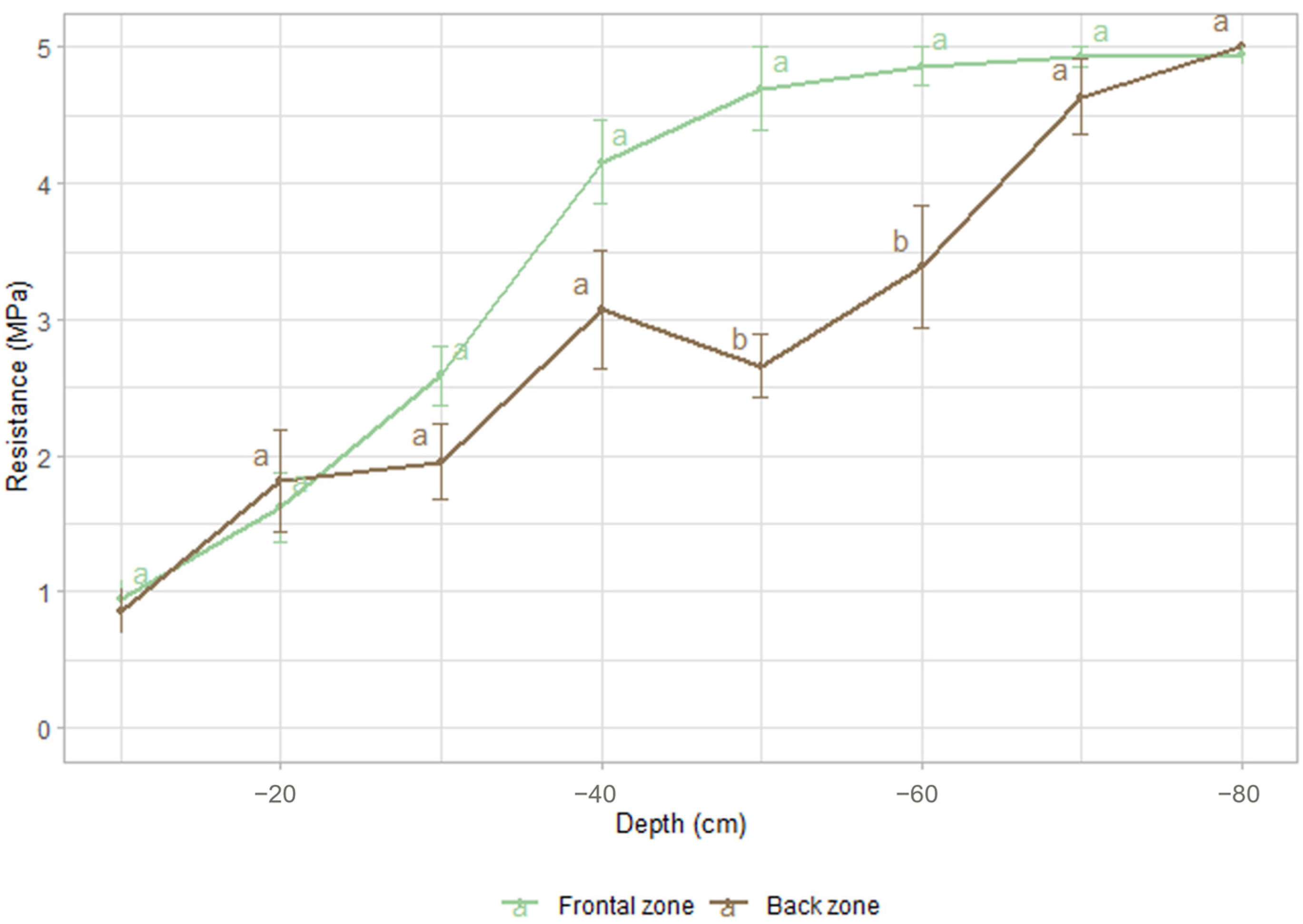
2.2. Soil Characteristics

The soil profile can be identified as an Arenosol according to World Reference Base classification. A homogeneous experimental field was assumed, but a gradient in the experimental field was visually observed based on a difference in plant growth by the researchers as by expert growers, with the front zone resulting in better growth compared to the back zone under the same fertilization conditions and independent of irrigation treatments. Several soil analyses were conducted to explain the soil gradient. Some differences in soil texture (according to USDA classification), total organic carbon, pH-KCL, magnesium, and calcium content were observed (Table 1).
Apparent electro-magnetic induction was measured on 24 November 2021 with aid of a soil scanner that applies electro-magnetic induction on one transmitter coil and four receiver coils. Apparent electrical conductivity was higher in the back zone compared to the front zone. This difference can be explained by the difference in altitude between both zones. The soil surface of the back zone was 10 cm lower than the front zone and, thus, closer to the shallow ground water table.
Via a penetrometer (Eijkelkamp, The Netherlands; 2 cm2 cone), soil resistivity (MPa) was determined every 10 cm till −80 cm depth at five different locations in both the front zone and back zone. A significant higher resistance was found in the front zone from −50 cm depth compared to the back zone (Figure 1). Because of the presence of the gradient, the location of the irrigation treatments in the field was switched between the two trials so that each treatment was once positioned in the front and once in the back zone.
Generally in the field, a shallow ground water was present, which was about −1.1 and −1.4 m below the soil surface at the beginning of spring and between −1.5 and −2 m below the soil surface at the end of summer. Depth of the groundwater table was recorded manually every month with the aid of a piezometer.
The soil’s water retention curve (pF) was determined at the start of the trials in 2022 and 2023, by undisturbed soil samples of 100 cm³ (Kopecky rings). In one plot per treatment, three samples were collected at a depth of −15 cm. Samples were used to measure bulk density and soil water retention points on pF 0 (0 kPa), pF 2 (−10 kPa) pF 2.7 (−50 kPa), and pF 4.2 (−1584 kPa). Water retention characteristics were acquired using pressure plates in the laboratory according to ISO NBN EN 11274 [24]. Other points on the water retention curve were interpolated with the aid of a polynomial regression. There was a slight variation in water retention characteristics over the two experimental years. The water-holding capacity of the soil can be defined as the fraction of soil water withheld between pF 2 and pF 4.2. In 2022, this fraction was higher in the irrigation treatment while it was the other way around in 2023. This makes sense since the location of the treatments was shifted between the years to exclude the effect of the field gradient (Table 2).

2.3. Soil Moisture Measurements

Soil moisture content (vol%) was continuously measured with Teros-10 soil capacitance sensors (METER group, USA) at −15 cm depth to be able to monitor the soil water content of the upper soil layer (0–30 cm) most affected by irrigation. Three sensors per treatment were installed, spaced 30 cm from each other. Each sensor was connected to a communication module that sends the observed field data to the cloud using the Sigfox LPWAN network. Sensors were calibrated with the aid of two specific soil samples to improve their accuracy. These destructive, composite samples were taken with a gauge auger in the soil layers of 0–30 cm. Calibration of the raw sensor measurement was performed by adding the average difference with the respective soil sample.

2.4. Soil Water Balance Model (SWB)

A classical soil water balance model, for example BUDGET [25], calculates the root zone depletion for the simulation period (Δt = 1 day) by considering the measured soil water content in the root zone at day i (Di), the daily rainfall (R), irrigation (I), estimated capillary rise (CR), and the crop evapotranspiration, which is calculated by multiplying reference evapotranspiration (ETo) with the crop coefficient Kc [13]. Deep percolation (DP) is considered when soil water content exceeds field capacity:
Di [mm]= Di−1 [mm]+ R [mm] + CR [mm] − DP [mm] + I [mm] − Kc ETo [mm]
The model used in our study builds upon this classical framework, is written in an R code, and has previously been described and used to calculate soil water dynamics in pear orchards [26] and strawberry fields [27]. Further specifications and differences with BUDGET [25] are described in Appendix A. The soil water balance model has been used by the Soil Service of Belgium to schedule irrigation on hundreds of farms in Belgium on a yearly basis since 2006. A detailed description of the model is added in Appendix A.
The daily ETo was calculated according to Penman–Monteith [13] based on observations of temperature, relative humidity, wind speed, and hours of sunshine collected at a weather station in Semmerzake, 18 km from the experimental site. The station is part of the observation network of the Royal Meteorological Institute of Belgium. Rainfall was collected on site.
In the SWB, field capacity is assumed at pF 2.1. Reduced actual evapotranspiration (ETa) due to drought stress, and closing of the stomata, is assumed at pF 2.5. The rooting depth of the crop was assumed to be 30 cm continuously over the entire growing season. The Kc factor that relates ET0 with maximal crop evapotranspiration ETc was assumed to evolve from 0.3 to 1.1 (Figure 2). Due to the lack of specific crop coefficients in the literature, an assumption was made based on the evolution of soil cover during the growing season. At planting there were no leaves at the trees, while soil cover in the plant beds was 100% at the end of the observation period at the start of October. The Kc factor was adjusted for evaporation. The first seven days after a wetting event, an increased potential ET is assumed according to the Equation (A5), according to the procedure described in Appendix A.
The SWB was calibrated with the Teros-10 sensor data. The coefficient of determination (R2) between observed and modelled water content was calculated just as the root means squared error (RMSE) (Equation (2)) and the Nash–Sutcliffe model efficiency coefficient (NSE) (Equation (3)). The root mean square error (RMSE) measures the average difference between a statistical model’s predicted values and the actual values and is expressed in units of soil water content (mm). NSE is an indicator that describes the predictive power of a model. In the situation of a perfect model with an estimation error variance equal to zero, the resulting Nash–Sutcliffe Efficiency equals 1.
R M S E = 1 n i = 1 n θ i ^ θ i 2
N S E = 1 i = 1 n θ i ^ θ i 2 i = 1 n θ i ^ θ o 2
In these equations, θ ^ is the SWB-predicted plant available water (mm), θ i is the Teros-10-observed plant available water (mm), θ o is the average observed plant available water (mm) with the Teros-10 sensor over the entire observation period, n is the amount of days over which the soil water storage times series is considered.

2.5. Irrigation

Water was supplied by a sprinkler irrigation system (Eindor 961/120) with a discharge of 120 L·h−1. Irrigation treatments were installed per experimental unit. The experimental units were spaced 20 m from each other to overcome interference of irrigation treatments. In the growing season of 2022, an irrigation treatment was located in the front and a rain-fed treatment in the back zone of the field. In 2023, the position of the treatments was switched to exclude any effects from the soil gradient present in the field (see Section 2.2). The irrigation was based on the predictions of the soil water balance model and was initiated when the total fraction of plant available water in the soil was depleted.

2.6. Plant Physiological Responses

In this study, the midday stem water potential (MPa) was determined each month, on the same day when soil samples were taken, with a pressure chamber (PMS Instrument, Wokingham, UK). To balance the water potential in the xylem of the leaf with the water potential in the xylem of the stem, leaves were enclosed in bags made of aluminum foil at least 1.5 h before sampling to be able to stop leaf transpiration [19,20]. Measurements were destructively performed on one leaf per tree and four trees per treatment.
In the growing season of 2023, continuous measurements of stem diameter variation using linear variable displacement transducers (LVDT; DF-5 series, Solartron Metrology Ltd., Steyning Way, UK) were performed on six trees, three trees of the rain-fed treatment and three trees of the irrigation treatment. In the rain-fed treatment, only two LVDT sensors recorded stem growth due to technical problems of the third sensor. One of the two working sensors also had technical problems for a 10-day period in June. In the irrigation treatment, all sensors were registering, but for two weeks in July growth was monitored by only two sensors. The sensors were calibrated prior to the experiments by measuring the signal in voltage at a known displacement of the sensor resulting in a linear regression between the voltage and the known displacement with R2 > 0.979 for each sensor, to be able to convert the raw voltage data into stem diameter variations (mm). The continuously measured stem diameter variations were used to calculate stem diameter growth, as the difference between the stem diameter variation measured at the start of the measurement campaign and at the moment when growth was determined.

2.7. Morphological Parameters

The length of 120 trees per treatment was monthly measured with a folding meter to follow up the growth increase. The tree length is used to sort the trees into commercial grading ranges after grubbing. Each month on the same day the length was measured; four (2022) or eight (2023) trees were harvested by cutting the stems just above the ground to determine fresh and dry weight and calculate LAI. The latter was achieved by measuring the total green canopy leaf area per unit surface area (estimation of 375 cm2 per tree based on the planting distances). The dry weight was obtained by heating the samples (stem and leaves) at 70–90 °C for at least one week.

2.8. Statistical Analyses

Statistical analysis was performed using Rstudio (R version 4.3.0) [28], complete with packages for making graphs [29,30,31,32]. If the data complied with normality and homoscedasticity, the two treatments, the rain-fed and irrigation treatment, were compared by a Student’s tt-test (p ≤ 0.05). Non-parametrical data were analyzed by a Mann–Whitney–Wilcoxon test (p ≤ 0.05). All results were expressed as means ± standard error (SE).

3. Results

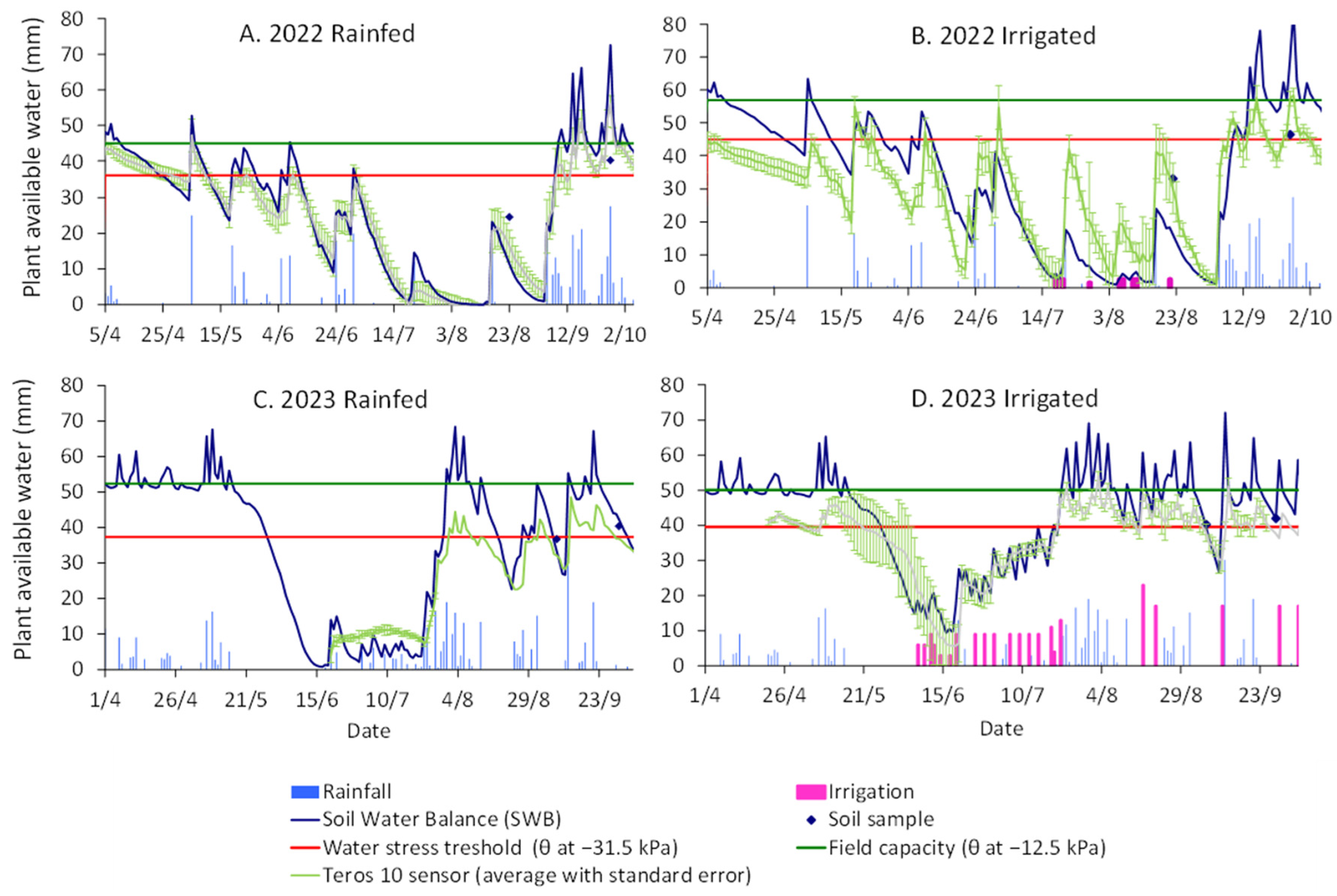
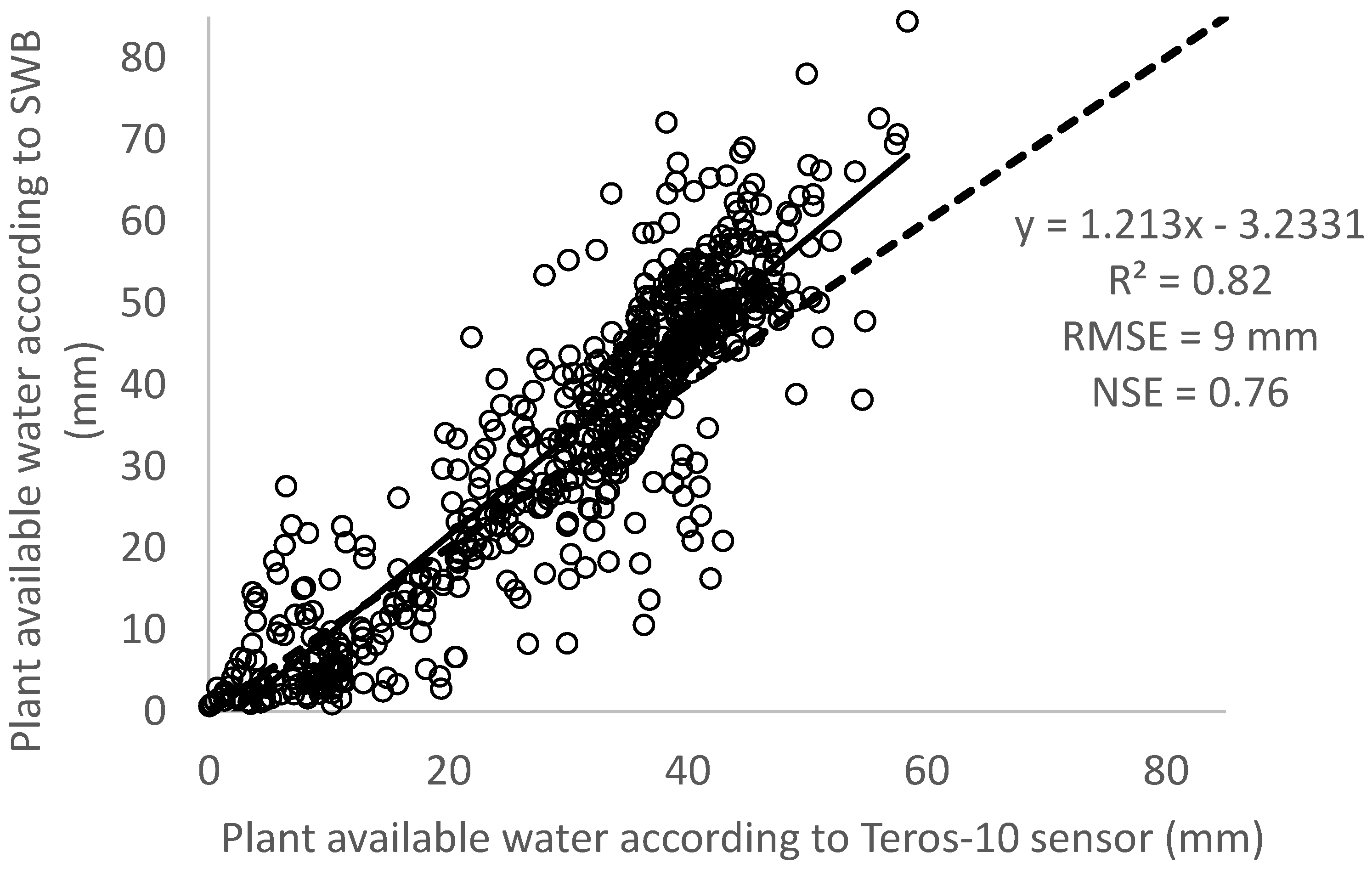
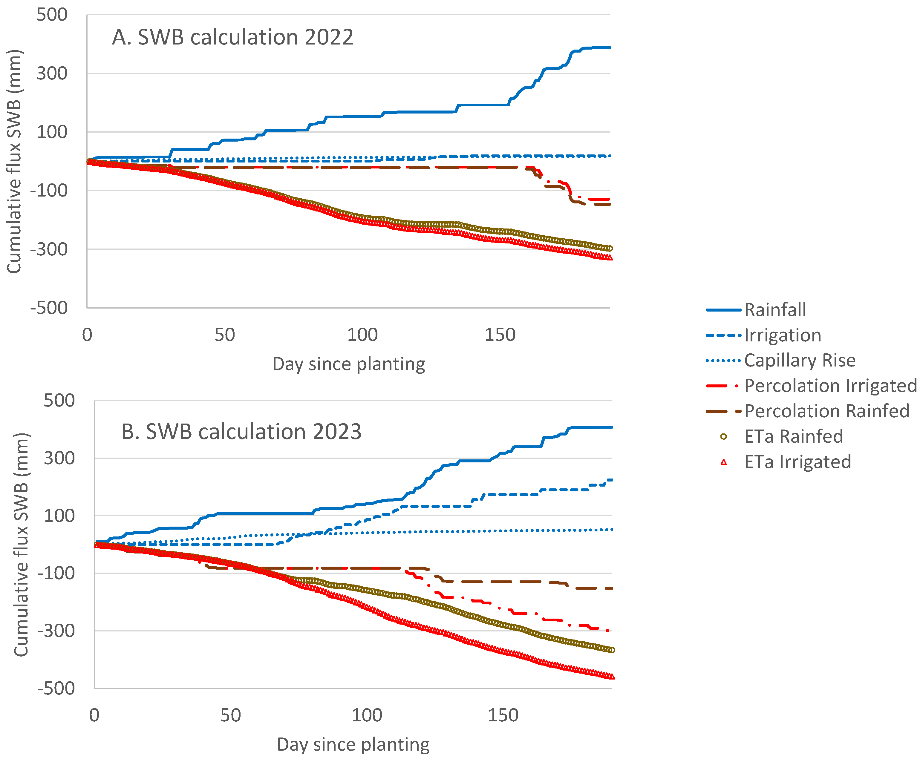
3.1. Soil Water Balance Calculation

The dynamics of plant available water could be acquired with aid of the SWB (Figure 3 and Figure 4). The SWB agreed reasonably well with the observed water content. The NSE was positive, RMSE was lower than 10 mm, which is about 0.03 m3·m−3 in a root zone of 30 cm. In nearly all treatments, there was a considerable variation between the three soil sensors. Only in 2023 in the rain-fed treatment, there was barely any variation. In this trial. there was a breakdown of the Teros-10 sensor module located in the irrigation treatment and data are only available from mid-June onwards.
In 2022, the plant available water was depleted in the beginning of July and irrigation was then initiated in the irrigation treatment. In total, 19 mm was irrigated, mainly until the end of August. In 2023, the plant available water was depleted in mid-June. Irrigation was maintained at a higher rate during the months of August: in total, 224 mm was irrigated.
The difference between rainfall and ETo was lower in 2023 (Figure 5, Table 3) than in 2022. The groundwater table was closer to the soil surface and there was more irrigation in 2023 compared to 2022, which led to a higher ETa but also to a higher ETa·ETc−1. Irrigation had a positive effect on ETa in both 2022 and 2023. While the effect of irrigation on ETa was limited in 2022, it had a big impact on ETa in 2023. In the irrigation treatment, ETa was 91 mm higher, which is 40% of the total irrigated amount.
In 2023, higher irrigation, rainfall, and capillary rise led to higher water percolation out of the root zone compared to 2022. In 2022, total percolation was quite similar between the irrigation and the rain-fed treatment, while in 2023 there was a big difference. In 2023, there was 147 mm pore percolation out of the root zone in the irrigation treatment compared to the rain-fed treatment, which is 65% of the total amount of irrigation. Percolation was high in 2023 due to the abundant, and rather unpredictable, rainfall in the second part of summer.

3.2. Effect of Irrigation on Midday Stem Water Potential

In 2022, during the months of April, May, and June, there was no irrigation. In this period, the stem water potential between the two treatments was more or less equal (Figure 6A). From the end of June, irrigation was started in the irrigation treatment. The stem water potentials began to differ between the rain-fed and the irrigation treatment, so irrigation also had an effect at plant level, but the differences were not significant. An additional measurement of stem water potential was taken on 9 August 2022, because the trees showed visible symptoms of drought and heat stress at that time. The stem water potential of the rain-fed treatment dropped to −1.85 ± 0.28 MPa. By irrigating the trees, the stem water potential of the irrigation treatment remained −1.18 ± 0.14 MPa. From September 2022, the dry period stopped and sufficient precipitation fell. From this month, the differences in stem water potentials between the treatments were minimized.
In 2023, during the dry weeks in June and early July, a difference in midday stem water potential was visible (Figure 6B). Irrigated trees had a less negative stem water potential value compared to the rain-fed treatment, which was already slightly stressed, especially on 13 June 2023 and 19 June 2023. On 19 June 2023, irrigation seemed to exert its effect where the irrigated trees had a midday stem water potential of −1.29 ± 0.38 MPa compared to a stem water potential of −2.48 ± 0.37 MPa of the rain-fed treatment. The difference between the treatments in midday stem water potential was not significant despite the hot and dry summer day of 19 June 2023. The stem water potentials differed significantly when determined on 17 July 2023, with the irrigation treatment having a value of −0.58 ± 0.04 MPa, and the rain-fed treatment having a value of −1.34 ± −0.12 MPa. From then on, irrigation barely had any effect on midday stem water potential, with no significant differences detected between treatments.

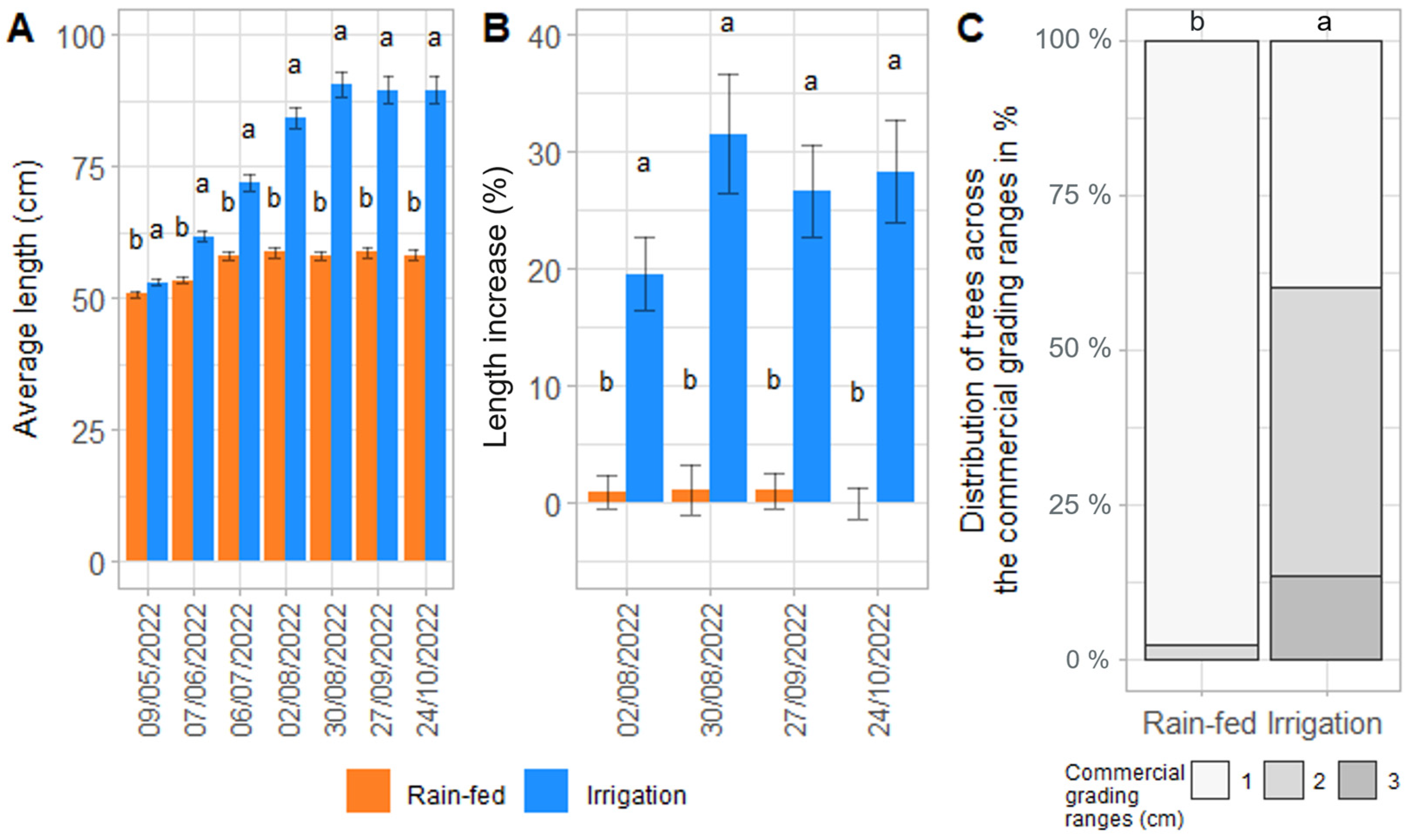
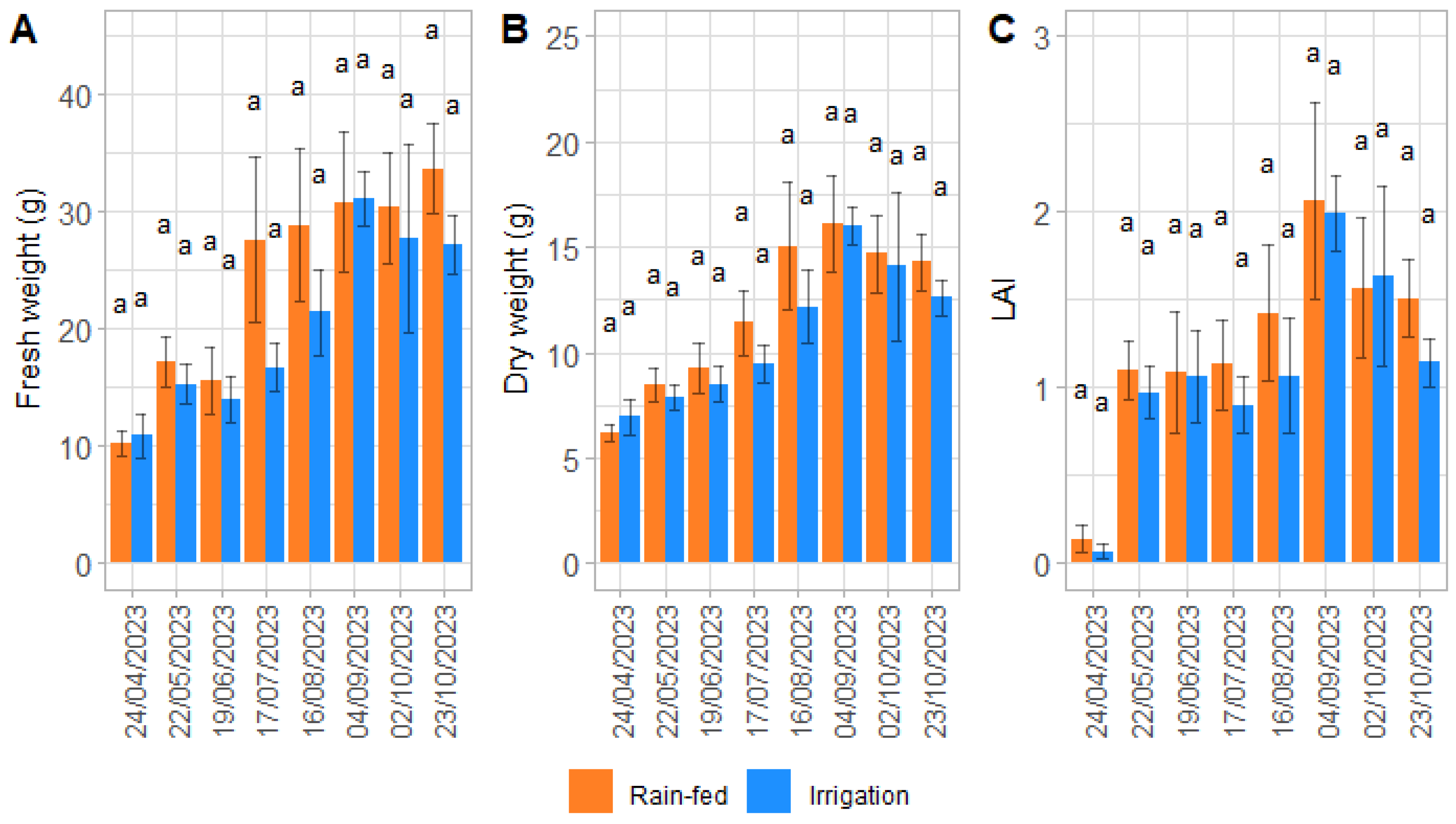
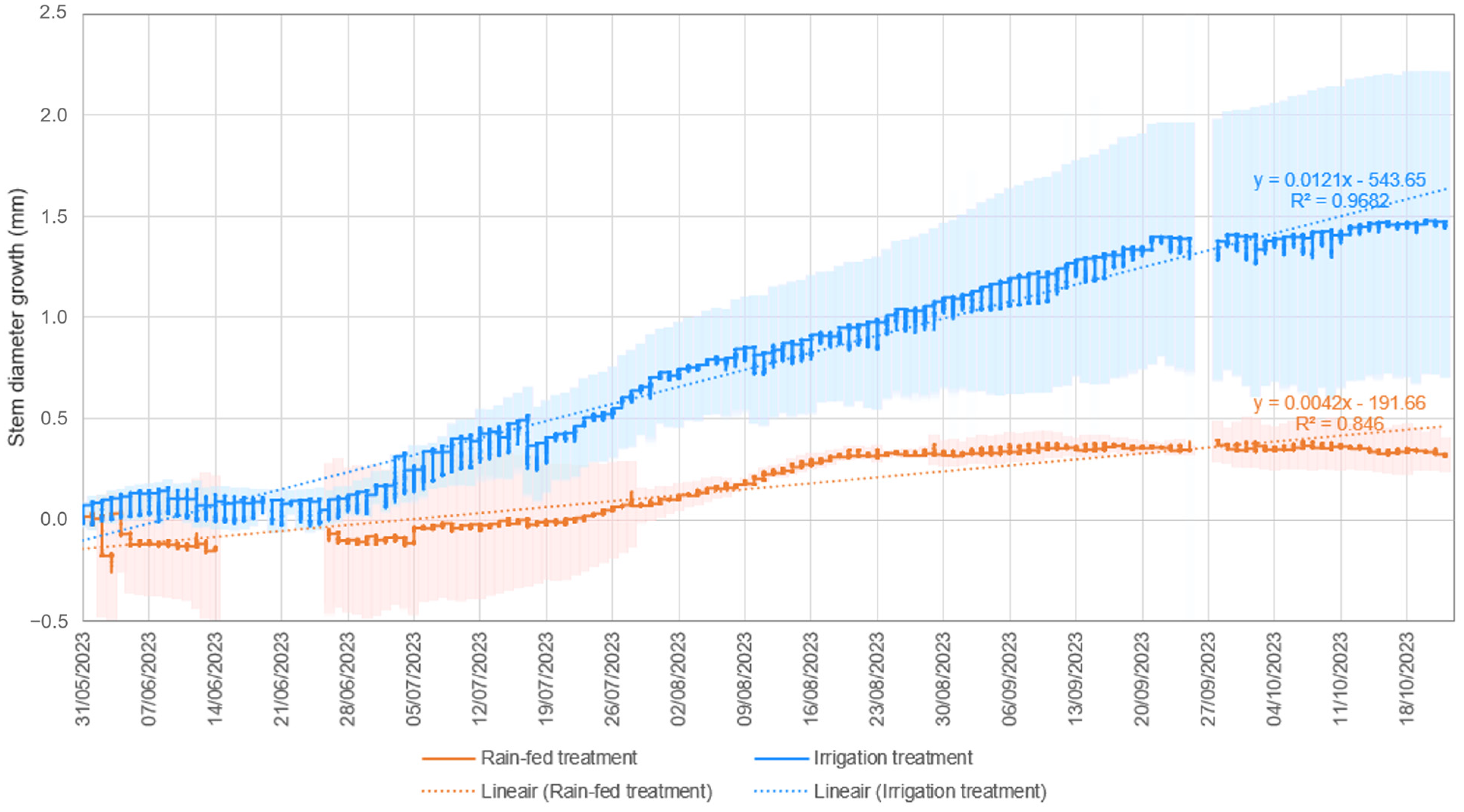
3.3. Effect of Irrigation on Plant Growth and Quality

Monthly, four trees of both treatments, the irrigation treatment and rain-fed treatment, were harvested and their fresh and dry weight and LAI were determined (Figure 7). Heavier plants with higher LAI were measured in the irrigation treatment from the beginning of July on 6 July 2022, even before irrigation started, although the differences were not significant (FW: rain-fed treatment 37.0 ± 6.6 g—irrigation treatment: 55.0 ± 5.2 g; LAI: rain-fed treatment 1.70 ± 0.36—irrigation treatment 2.79 ± 0.54). This observation raised the suspicion of a gradient in soil conditions across the field (as described in Section 2.2), with the irrigation treatment oriented in the front and more optimal zone of the field in 2022. The irrigation treatment had a positive effect on the trees and further increased the difference in biomass between the treatments at the beginning of August, although the standard error is high as only four measurements were performed per treatment (rain-fed treatment: 37.3 ± 11.0 g; irrigation treatment: 71.1 ± 20.7 g). From then, weight and LAI decreased again, which can be explained by the effect of the drought and heat period in early August, which advanced the autumn leaf fall.
The effect of the soil gradient can also be seen on plant length at the time of the first measurement, where a significant difference between the treatments is present (Figure 8A). Irrigation started in mid-July had an additional effect on tree growth and further increased the difference in length between treatments. On 30 August 2022, the irrigated trees had an average length increase, compared to the tree length before the start of irrigation on 6 July 2022, of 70.5% compared to a length increase of 15.5% of the rain-fed trees. The growth in length since the start of irrigation is shown in Figure 8B. There was still growth in August after the growth spurt in June and July, the moment in the season of strongest growth, but it declined and stopped from September. The trees in the rain-fed treatment stopped growing earlier, since they had less water available from mid-July. At harvest, forest trees are sorted according to their length into commercial grading ranges. The effect of the treatments on this grading was also assessed (Figure 8C). Irrigation combined with optimal soil quality conditions in the front zone of the field had a significant effect on grading with more trees in higher grading ranges. The irrigation treatment had 13% of trees sorted in the commercial grading range 3 (125–150 cm), while in the rain-fed treatment, no trees were sorted in this grading range. In the rain-fed treatment, 97.5% of the trees were sorted in the lowest grading range (50–80 cm) compared with 40% of the trees in the irrigation treatment.
Monthly, four trees were harvested for each treatment and their fresh and dry weight and LAI were determined (Figure 9). Before the start of the irrigation treatments (until 19 June 2023), hardly any differences between the treatments were observed. During the measurements in July and August, it is noticeable that the rain-fed treatment received a huge growth spurt despite the drought and the fact that this treatment did not receive irrigation (28.9 ± 6.5 g for the rain-fed treatment compared to 21.4 ± 3.7 g for the irrigation treatment, measured at 16 August 2023), explainable by its location in the field. Irrigation still allowed these trees to catch up with the growth lag at the beginning of September. This catch-up disappeared again the moment leaf fall began to occur in autumn, and from then on the rain-fed trees had more biomass and a higher LAI. It was also visually observed that leaf fall started later in the rain-fed treatment and so the front zone of the field.
The effect of the soil gradient was already visible from bud burst in spring, resulting in taller trees in the rain-fed treatment (see measurements 24 April 2023 and 22 May 2023, Figure 10A). Irrigation was started during the dry period in mid-June and the dose was increased in mid-July; from then on, it can be seen that the trees in the irrigation treatment caught up with their growth lag that had built up due to their location in the back zone of the field. From 16 August 2023, significant differences in length between the treatments disappeared. This is even more evident in Figure 10B, where the length increases relative to the measurement before the start of the irrigation treatments (22 May 2023) are depicted. The growth rate of the irrigated trees was significantly higher (20.6 ± 3.0% on 23 October 2023) compared to the growth rate of the rain-fed treatment on 23 October 2023 (14.8 ± 3.1%). At the end of the season, when the plants were harvested, the trees were divided into different grading ranges based on their length, with slightly more trees in range 1 (50–80 cm) for the irrigation treatment (21.7% compared to 16.7% of the rain-fed trees sorted in grading range 1) (Figure 10C).
In 2022, a strong effect of the irrigation treatment was observed on tree growth through the monthly length measurements. Therefore, we decided to install linear variable displacement transducer (LVDT) sensors in 2023. This allowed continuous monitoring of tree growth in terms of stem diameter and cumulative stem growth so the effect of irrigation could be analyzed more in depth. From the start of irrigation in mid-June, we saw that the cumulative stem diameter growth of the irrigated trees (slope of the blue curve) became greater than the stem diameter growth of the rain-fed trees (slope of the orange curve), meaning that irrigation immediately exerted a positive effect (Figure 11). A linear regression was fitted through both curves to quantify the difference in growth (dotted lines). It can be stated that the cumulative growth in the irrigated trees (direction coefficient of 0.0121) was three times that of the rain-fed trees (direction coefficient of 0.0042). Continuous monitoring of tree growth also showed that the growth decreased and stopped in August in the case of the rain-fed treatment, but continued due to irrigation in the irrigation treatment until mid-September. Irrigation resulted in a cumulative growth of 1.5 mm compared to only ± 0.3 mm in the rain-fed treatment.

4. Discussion

A calibrated SWB gives insight in the crop response to low soil moisture. The SWB links a low soil water status to reduced ETa and, thus, lower biomass production. The calculations of the SWB agreed quite well with the observed plant available water content. Agreement was better than previous efforts to link calculated soil water potential with observations of granular matrix sensors in pear orchards [33]. This can be explained due to the fact that in the current experiment, Teros-10 sensors were used, which measure soil moisture instead of soil water potential measured with Watermark sensors, and that the sensors were calibrated with in situ moisture samples. The observed NSE was comparable to the SWB calculations in strawberry plants where comparison was made with in situ soil moisture samples rather than sensor measurements [27].
The SWB was well calibrated but uncertainty about its underlying processes is inherent in any SWB. For example an overestimation of evapotranspiration may be compensated by an overestimation of capillary rise. Parameters like rooting depth, evaporation, transpiration, and soil hydraulic properties are highly variable and can only be measured to a certain extent. A view on the different fluxes in the soil water balance learned that when a high amount of irrigation was applied, like in 2023, that then 65% of the total amount of irrigation percolated out of the root zone. Despite this high amount of percolation, ETa was still 10 mm lower than ETm. In previous SWB calculations, increased irrigation was also linked to higher percolation [34,35,36]. The SWB calculation clearly shows that the rain-fed treatment suffered from drought stress in accordance with the plant observations. In the SWB, stress was assumed to start at pF 2.5. Previous experiments that link soil water potential to water stress in ornamental trees grown in the open field are lacking. In Mediterranean environments, water stress has been observed at pF 2.3 for pear [37], pF 2.6 for plum [38], and pF 2.7 for apple [39]. In the Belgian temperate climate, yield decline for pear was observed at pF 3 [40]. To assure the profitability of an irrigation event in A. pseudoplatanus, it is advised to start irrigation at mild water stress, which is expected to occur between pF 2.6 and pF 2.9.
Plant-based methods for irrigation control, e.g., determination of leaf or stem water potential, can be used as plants might respond directly to changes in water status in their plant tissues rather than to changes in soil water content [15,16,22]. However, determination of the leaf or stem water potential at solar noon cannot be used to evaluate and monitor soil water content itself, relative to the predawn measurement of stem water potential. Yet, the determination at solar noon will still indicate whether a plant or tree is under stress and not adequately irrigated [41,42]. In this study, irrigation exerted a positive effect on midday stem water potentials, resulting in less negative values. At the driest and warmest moment in 2022, in early August, the stem water potential of the rain-fed trees dropped to −1.84 ± 0.28 MPa, while the potential of the irrigated trees dropped only slightly below −1 MPa. During the dry period in June 2023, the stem water potentials of the rain-fed trees reached values around −3 MPa, as did the stem water potential of the irrigated trees. The irrigation dose was still not sufficient at this time, as the soil moisture still decreased despite the first irrigation doses in June. Irrigation rate was, therefore, increased in July 2023. The increase in irrigation dose was also reflected at plant level. By mid-June 2023, the expected effect of the irrigation treatment on stem water potential was observed, with the rain-fed trees having the lowest stem water potential of −2.48 MPa and the irrigated trees a potential of −1.29 MPa. McDonald, 1984, described in his forest nursery manual that tree seedlings will be stressed at plant water potentials between −1 and −1.5 MPa, irrespective of species [41]. This threshold cannot be fully adopted, since our study tested irrigation treatment on 1 + 0 transplants and not on seedlings. Previously, irrigation research specific to A. pseudoplatanus was mainly conducted on potted Acer trees grown under protection, in which leaf water potentials were measured. Overall, irrigation had no discernible effect on leaf water potential with no significant differences observed between the non-irrigated and irrigated trees [5,10,43]. Leaf water potentials are more variable and, thus, more difficult to compare with the stem water potentials measured in our study. Keller et al. (2024) studied Acer rubrum trees grown in soil under drought and well-watered conditions. Stem water potentials reached values of −1.2 MPa under drought conditions [44]. Most previous research on irrigation scheduling has been conducted in soil-grown fruit orchards, where stem water potential has typically been measured at solar noon, allowing for comparison with our study. Midday stem water potential of well-irrigated apple [45,46,47], pear [48], peach [22,49], prune [20,50], almond [51,52], grapevine [46,53], and raspberry [54] trees varied between −0.5 and −1.0 MPa. From these studies, it can also be concluded that under drought stress conditions, stem water potential decreased to levels below −1.5 and −2.0 MPa depending on the drought stress tolerance of the species. These values are lower than those observed by Keller et al. on Acer rubrum [44] and described by McDonald for forest tree seedlings [41]. Based on these studies, it can be said that the irrigated Acer trees did not experience drought stress compared to the rain-fed treatment during dry periods, at least based on the midday stem water potentials. Determination of stem water potential is an intensive measurement techniques that is also a snapshot in time, making it less suitable for irrigation control by the growers themselves. However, these measurements will help us with further finetuning the irrigation thresholds at soil level in future.
Irrigation also exerted a positive effect on tree growth in both trial years. In the drier year of 2022, irrigation stimulated growth with 28.4% compared to the rain-fed treatment, and with trees being sorted into higher commercial grading ranges and, thus, on average, having a higher commercial value. In 2023, irrigation resulted in only 5.8% more growth compared to the rain-fed treatment. This smaller effect can be explained by two reasons. On the one hand, 2023 was wetter compared to 2022 (see Appendix B, Table A1 and Table A2), theoretically requiring less irrigation. Nevertheless, due to finetuning of the model, more irrigation was applied in 2023 than in 2022, suggesting that factors beyond water supply also have an effect on tree growth. As described in Section 2.1, a homogeneous experimental field was assumed but proved not to be the case by visual assessment of tree growth and analysis of the soil. Apparent electrical conductivity, acquired with the soil scanner, was different between both zones. The front zone of the experimental field appeared to have more optimal soil quality conditions with a slightly higher pH, total organic carbon, magnesium, and calcium content. and a fine sand soil texture compared to the back zone of the field (Table 1). However, these conditions ensured that irrigation could exert an additional effect in 2022 when the irrigation treatment was applied in this apparent more optimal front zone of our experimental field. In 2023, the treatments were switched positions, with the irrigation treatment being applied in the back and less optimal soil quality zone of our experimental field. This location limited the effect of irrigation to only 5.8% more growth. Yet, irrigation successfully mitigated the less favorable growth conditions in the back zone of the field, resulting in tree growth similar to that in the rain-fed treatment in the more optimal zone.
Hipps et al. (1996) assessed the effect of a low and high irrigation rate on the growth of A. pseudoplatanus seedlings [8]. The high-rate irrigated trees were double in length and had ±60% increase in seedling dry weight and an increase in total leaf area linked with higher LAI. In our study, the direct effect of irrigation was more limited. However, since irrigation regimes were tested on transplanted seedlings (1 + 0), direct comparison is challenging. This is consistent with the findings of Fini et al. (2007), who reported no effect of irrigation on plant height of A. pseudoplatanus [9]. However, in one of their trials, irrigation significantly enhanced shoot elongation compared to the non-irrigation treatment [8]. The set-up of irrigation and drought experiments in containers and greenhouses are more predictable, as climate conditions and growing medium can be controlled, as demonstrated by Koç [7] and Fini et al. [10]. In the study of Koç (2022) on 2-year-old A. pseudoplatanus in containers, the well-watered trees were 34.8% taller compared to the trees grown under reduced irrigation [7]. In the experiment of Fini et al. (2008), A. pseudoplatanus trees grown in 3 L containers filled with peat and perlite were subjected to two irrigation treatments: normal irrigation vs. reduced (50%) irrigation. However, it was observed that the irrigated trees were 30.5% smaller and had 38.4% less shoot dry weight compared to the reduced irrigated trees, although these differences were not significant. They explained this contradictory observation by the fact that the normal irrigation regimes in tree nurseries are too high and would be better reduced for more optimal tree growth depending on the tree species [10]. Furthermore, already quite a bit of research has been conducted on other Acer species, such as A. rubrum, A. x freemanii, and A. campestre but comparison with A. pseudoplatanus is not always obvious as the different species will cope differently with drought. In the research of Fox and Montague (2009), three irrigation regimes (100, 60, and 30% ETo) were tested on different Acer species [55]. For the A. x freemanii and A. truncatum, the 60% ETo treatment gave the best effect on shoot elongation, compared to A. campestre, which responded best to the 30% ETo treatment. This species is known to be more drought tolerant. Also in another study, A. x freemanii responded best on the 60% ETo irrigation dose [56]. Irrigation studies were also already performed on A. rubrum. Ponder et al. (1984) found significant effects of 100 and 50% irrigation treatments on tree growth in length (+9.5%) at the end of the growing season compared to the non-irrigated trees, with no significant difference between the 100% and 50% deficit irrigation treatment [57]. In general, irrigation exerts a positive effect on growth, especially under drought conditions, also in our study. Further research will determine the reduction in growth at the critical irrigation threshold at soil level, so that growers will be able to control their irrigation based on this growth parameter.
Even though forest nursery plants are sorted according to their length, in 2023, we assessed continuous measurements of swelling and shrinking of the stem and stem diameter growth with LVDT sensors. Measurement with this sensor is interesting because it allows detection of when and how fast growth responds to irrigation [58,59]. From our study, it can be concluded that the growth of rain-fed A. pseudoplatanus decreased from mid-August as daylength shortened. Irrigation had an additional effect and delayed the decrease in and cessation of stem growth until September. Irrigation applications in September (Appendix B, Table A2) no longer had any effect on growth. It can be inferred that even if the weather still appears to be vigorous in the late summer months, September and October, irrigation no longer had any additional effect on growth of Acer pseudoplatanus as the trees prepare for winter dormancy. In another study on older A. pseudoplatanus trees in a mixed forest in Germany, Köcher et al. (2012) installed dendrometers to analyze the influence of rainfall, soil moisture, air humidity, atmospheric vapor pressure deficit, air temperature, and global radiation on stem radius changes [60]. The stem diameter increment started mid-May and decreased from the middle of August, comparable with our study. Valdovinos-Ayala et al. (2022) installed several dendrometers on A. rubrum trees in a common garden [61]. Every 2–3 days, the trunk diameter was measured by the dendrometers so that growth could be determined. They too determined that trunk diameter growth of A. rubrum stopped from mid-August onwards, 2.5 months before full leaf fall of the trees. The strongest stem diameter growth was observed in the months of May and June. In our experiment on A. pseudoplatanus, the strongest growth in stem diameter occurred in June–July, as we studied another Acer species grown under a different climate. Ponder et al. (1984) determined also the effect of different irrigation treatments, 0, 50, and 100% irrigation, on the cumulative trunk diameter increase of A. rubrum [57]. Irrigation positively influenced stem diameter growth with continued growth until November, while growth of non-irrigated trees decreased from August and stopped from September. There was little difference between the 50 and 100% irrigation treatment, with the 100% leading to slightly more growth (not significant). Garnier and Berger, 1986, studied the effect of 50% and 100% irrigation on peach trees and measured the daily stem diameter growth [62]. They observed that cumulative stem growth was not much affected by the 50% deficit treatment until mid-July, while stem diameter growth continued longer in the 100% irrigated trees.

5. Conclusions

This study concludes that the rain-fed treatment suffered from drought stress at pF 2.5, based on the SWB calculation, in accordance with the plant observations. From an economic point of view, it may be interesting to set a drier threshold, between pF 2.6 and 2.9, to trigger irrigation to guarantee that the benefit covers the irrigation cost. This drier threshold will also decrease the amount water percolation out of the root zone linked to irrigation. Sprinkler irrigation, based on the SWB calculation, in the cultivation of forest tree liners positively affected the growth and quality of 1 + 0 liners of Acer pseudoplatanus, with growth increases of 28% and 6% in 2022 and 2023, respectively. The effect of irrigation will be year-dependent, given the difference in climate conditions between years, but will also be plant-dependent. Additionally, irrigation could delay the decrease in and cessation of stem growth until September compared to a stop in stem growth from mid-August in the case of the rain-fed treatment, but the application in September no longer had any effect on growth as the trees prepared for winter dormancy. Improved growth with irrigation was accompanied by higher (less negative) midday stem water potential, indicating the absence of stress conditions.

Author Contributions

Conceptualization, M.-C.V.L., P.D.C., D.V.H., P.J. and K.S.; methodology, P.D.C., A.D.V., P.J., K.S., D.V.H., M.-C.V.L. and E.D.; software, P.D.C., A.D.V. and P.J.; formal analysis, P.D.C., A.D.V. and P.J.; investigation, P.D.C. and A.D.V.; data curation, P.D.C., A.D.V. and P.J.; writing—original draft preparation, P.D.C.; writing—review and editing, P.D.C., A.D.V., P.J., K.S., D.V.H., B.G., M.-C.V.L. and E.D.; visualization, P.D.C., A.D.V. and P.J.; supervision, E.D., M.-C.V.L. and K.S.; project administration, P.D.C.; funding acquisition, M.-C.V.L., P.D.C., D.V.H., P.J. and K.S. All authors have read and agreed to the published version of the manuscript.

Funding

This research was conducted in the framework of the OrnAqua project (a new irrigation reference framework for increasing water use efficiency in outdoor horticulture), which is a project funded by Flanders Innovation & Entrepreneurship (VLAIO). Project number: HBC.2020.3202.

Data Availability Statement

The raw data supporting the conclusions of this article will be made available by the authors on request.

Acknowledgments

The author wants to thank Lise De Clerck, Christophe Petit, and Simon Menu for their technical assistance on the field, and also the entire VLAIO LA OrnAqua consortium for the insights, support, and nice collaboration.

Conflicts of Interest

The authors declare no conflict of interest.

Appendix A. Description of the Soil Water Balance Calculation

A classical soil water balance model, for example BUDGET [25], calculates the root zone depletion for the simulation period (Δt = 1 day) by considering the measured soil water content in the root zone at day i (Di), the daily rainfall (R), irrigation (I), estimated capillary rise (CR), and the crop evapotranspiration, which is calculated by multiplying reference evapotranspiration (ETo) with the crop coefficient Kc [13]. Deep percolation (DP) is considered when soil water content exceeds field capacity:
D i   [ m m ] = D i 1   [ m m ] + R   [ m m ] + C R   [ m m ] D P   [ m m ] + I   [ m m ] K c E T o   [ m m ]
The soil water balance used in the experiment has the same basic algorithms as BUDGET [25].
The differences with BUDGET [25] are:
  • Field capacity was set at pF 2 and when soil water content exceeds field capacity, water drains out of the root zone to field capacity the day after. Field capacity was considered at pF 2 because there was a shallow ground water table present in Hoogstraten approximately at 100 cm below the soil surface. In Sint-Truiden, water was retained in the subsoil due to clay accumulation in the Luvisol soil type, which also supports the choice of setting field capacity at pF 2. It has been demonstrated that field capacity differs in function of soil texture, hydraulic conductivity, evapotranspiration, and rooting depth [63,64].
  • The soil water balance was for the entire growing season calculated for a single soil layer from 0 to 30 cm.
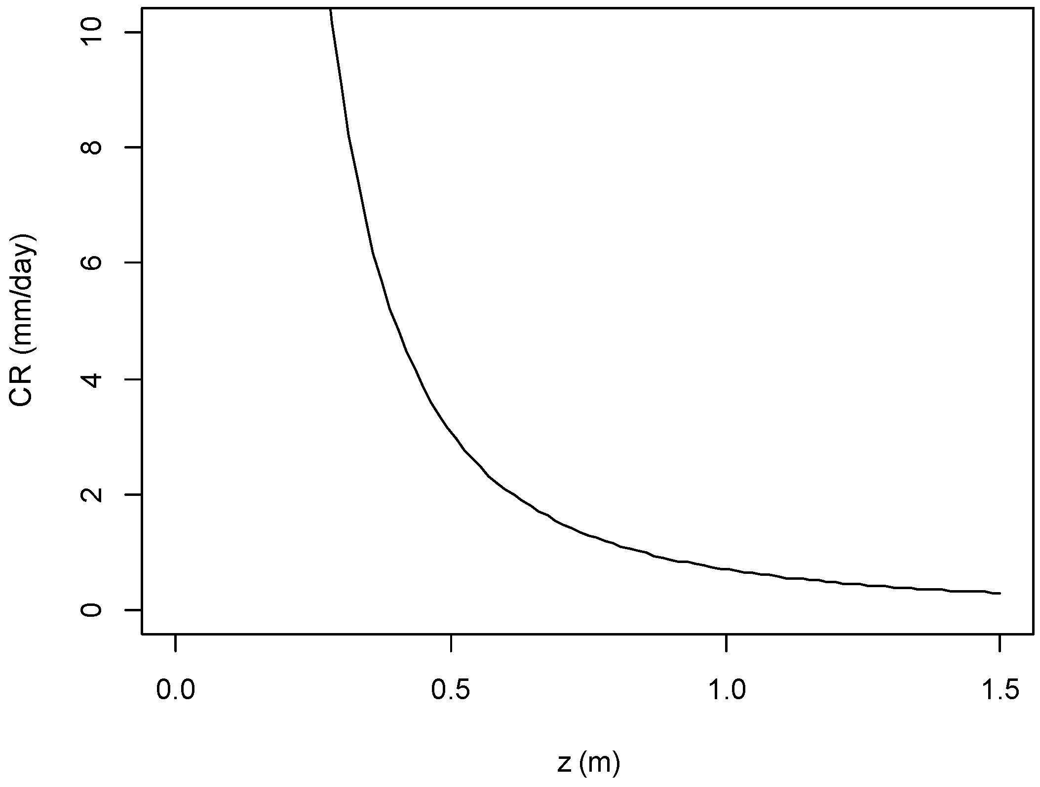
  • In the soil water balance model, capillary rise is calculated with empirical algorithms derived from UPFLOW [65], which calculates the capillary rise as a function of the groundwater table depth, and water retention characteristics. A similar approach was used in the water balance algorithms that underlie AquaCrop [66] (Equation (A2) and Figure A1).
    C R = e x p ( log z ( 0.32 ln K s a t 0.02 ) / ( 0.02 ln K s a t 0.2 ) )
With z: depth of ground water table (m), CR: capillary rise (mm·day−1), and Ksat: saturated hydraulic conductivity (m·day−1), which was assumed 0.8 m·day−1 in the current study.
Especially in Hoogstraten, there was a significant contribution of capillary rise due to the shallow ground water table. Capillary rise in Hoogstraten was expected to vary between 0 and 1.2 mm·day−1 depending from the ground water table depth, which was summarized to be about 75 to 120 mm·year−1.
Figure A1. Relationship between capillary rise and depth of ground water table used in the soil water balance calculation.
Horticulturae 11 00435 g0a1
4.
When Ψsoil drops below a critical Ψkrit of −31 kPa. an empirical relationship was used to define an exponential decrease in actual evapotranspiration (ETa) in relation to maximal potential evapotranspiration (ETc), similar to many other models [67] (Equation (A3) and Figure A2).
E T a E T m = 1 15500 ( 10 θ θ k r i t 1.5 w p θ k r i t + 2.7 16000 ) m
With ETa: actual daily evapotranspiration (mm), ETm: maximal daily evapotranspiration (mm·day−1), θ: soil moisture (cm3·cm−3), and θkrit: soil moisture threshold (cm3·cm−3) at which the plant suffers from water stress.
Figure A2. Effect of water stress, quantified by ETa·ETm−1 in function soil moisture when critical soil moisture is set at 0.25 cm3·cm−3.
Horticulturae 11 00435 g0a2
5.
After a wetting event, actual evapotranspiration will be dominated by evaporation and is calculated through a Ke factor (Equation (A4)). This Ke factor is related to the time after a wetting event in a curved empirical relationship (Equation (A5) and Figure A3). The first four days after the wetting event, Ke is close to 1, representing the stage I, whereby vaporization is controlled by capillary flow to the vaporization plane at the surface. After four days Ke decreases, representing stage II of vaporization where vapor diffusion is controlled [68].
E T a = E T 0 K e
K e = 0.25 + ( 1 0.25 ) ( 1 ( w 8 ) 5 )
With Ke: soil evaporation coefficient and w: days after soil wetting.
Figure A3. The soil evaporation coefficient (Ke) incorporated in the soil water balance model in function of time.
Horticulturae 11 00435 g0a3

Appendix B

Table A1. Weekly temperature, radiation sum, relative humidity, precipitation and irrigation during the 2022 trial.
WeekAverage Temperature (°C)Radiation Sum (W·m−2)Relative Humidity (%)Precipitation (mm)Irrigation (mm)
W18 (25/04)9.933,47279.50.60
W19 (02/05)13.636,91480.3250
W20 (09/05)16.642,19170.400
W21 (16/05)18.035,06380.121.80
W22 (23/05)14.529,65982.211.40
W23 (30/05)15.134,70178;617.20
W24 (06/06)16.830,75581.214.40
W25 (13/06)19.644,76072.620
W26 (20/06)18.635,69279.720.80
W27 (27/06)17.834,13279.724.60
W28 (04/07)18.239,59179.10.60
W29 (11/07)20.638,19173.000
W30 (18/07)21.834,75377.514.45.1
W31 (25/07)19.432,71777.51.21.7
W32 (01/08)21.234,13573.805.1
W33 (08/08)22.940,93365.505.1
W34 (15/08)20.524,95284.624.22.5
W35 (22/08)21.028,34080.302.5
W36 (29/08)19.726,51780.300
W37 (05/09)18.220,75989.358.20
W38 (12/09)14.614,99993.865.60
W39 (19/09)11.919,45391.712.40
W40 (26/09)11.614,15593.057.80
W41 (03/10)12.215,25888.82.20
W42 (10/10)11.512,21494.13.40
W43 (17/10)14.711,54894.810.40
W44 (24/10)15.411,72591.62.40
Table A2. Weekly temperature, radiation sum, relative humidity, precipitation and irrigation during the 2023 trial.
WeekAverage Temperature (°C)Radiation Sum (W·m−2)Relative Humidity (%)Precipitation (mm)Irrigation Treatment (mm)
W18 (24/04)9.828,55067.56.40
W19 (01/05)14.033,01266.9210
W20 (08/05)13.822,90180.126.80
W21 (15/05)13.038,67566.44.20
W22 (22/05)14.840,19864.000
W23 (29/05)16.350,46957.100
W24 (05/06)21.148,77255.7018
W25 (12/06)22.543,78050.50.621
W26 (19/06)21.739,26266.417.818
W27 (26/06)19.026,00864.65.818
W28 (03/07)19.934,06861.712.618
W29 (10/07)20.435,06561.310.619
W30 (17/07)18.030,32767.913.230
W31 (24/07)17.925,58474.243.40
W32 (31/07)16.319,84583.463.80
W33 (07/08)18.533,27971.217.20
W34 (14/08)20.630,83273.6015
W35 (21/08)18.924,65577.227.815
W36 (28/08)16.822,38880.622.40
W37 (04/09)22.031,19073.80.20
W38 (11/09)18.621,19581.737.417
W39 (18/09)15.615,84279.529.20
W40 (25/09)16.016,79879.91.217
W41 (02/10)16.516,29075.40.817
W42 (09/10)15.011,48880.826.812
W43 (16/10)12.010,38082.1330
W44 (23/10)10.810,35689.028.20

References

  1. Agentschap Landbouw en Zeevisserij. Productiewaarde Sierteelt. Available online: https://landbouwcijfers.vlaanderen.be/landbouw/sierteelt/productiewaarde-sierteelt (accessed on 10 December 2024).
  2. VLAM Marketingsdienst. Sierteeltbarometer 2022. Available online: https://www.flandersplants.com/sites/vlamfresh_floriculture/files/publication/file/Sierteeltbarometer%202022.pdf (accessed on 10 December 2024).
  3. Calvin, K.; Dasgupta, D.; Krinner, G.; Mukherji, A.; Thorne, P.W.; Trisos, C.; Romero, J.; Aldunce, P.; Barrett, K.; Blanco, G.; et al. IPCC, 2023: Climate Change 2023: Synthesis Report. Contribution of Working Groups I, II and III to the Sixth Assessment Report of the Intergovernmental Panel on Climate Change; Core Writing Team, Lee, H., Romero, J., Eds.; IPCC: Geneva, Switzerland, 2023. [Google Scholar]
  4. Carón, M.M.; De Frenne, P.; Brunet, J.; Chabrerie, O.; Cousins, S.A.O.; De Backer, L.; Decocq, G.; Diekmann, M.; Heinken, T.; Kolb, A.; et al. Interacting Effects of Warming and Drought on Regeneration and Early Growth of Acer pseudoplatanus and A. platanoides. Plant Biol. 2015, 17, 52–62. [Google Scholar] [CrossRef] [PubMed]
  5. Khalil, A.A.M.; Grace, J. Acclimation to Drought in Acer Pseudoplatanus L. (Sycamore) Seedlings. J. Exp. Bot. 1992, 43, 1591–1602. [Google Scholar] [CrossRef]
  6. Kunz, J.; Räder, A.; Bauhus, J. Effects of Drought and Rewetting on Growth and Gas Exchange of Minor European Broadleaved Tree Species. Forests 2016, 7, 239. [Google Scholar] [CrossRef]
  7. Koç, İ. Comparison of the Gas Exchange Parameters of Two Maple Species (Acer negundo and Acer pseudoplatanus) Seedlings under Drought Stress. Bartın Orman Fak. Derg. 2022, 24, 65–76. [Google Scholar] [CrossRef]
  8. Hipps, N.A.; Higgs, K.H.; Collard, L.G. The Effect of Irrigation and Root Pruning on the Growth of Sycamore (Acer pseudoplatanus) Seedlings in Nursery Beds and after Transplantation. J. Hortic. Sci. Biotechnol. 1996, 71, 819–828. [Google Scholar] [CrossRef]
  9. Fini, A.; Ferrini, F.; Frangi, P.; Amoroso, G. Growth and Physiology of Field-Grown Acer pseudoplatanus L. Trees as Influenced by Irrigation and Fertilization. In SNA Research Conference; Field Production: Columbus, OH, USA, 2007; Volume 52, pp. 51–55. [Google Scholar]
  10. Fini, A.; Mattii, G.B.; Ferrini, F. Physiological Responses to Different Irrigation Regimes for Shade Trees Grown in Container. Adv. Hortic. Sci. 2008, 22, 13–20. [Google Scholar]
  11. Bianchi, A.; Masseroni, D.; Thalheimer, M.; de Medici Leonardo, O.; Facchi, A. Field Irrigation Management through Soil Water Potential Measurements: A Review. Ital. J. Agrometeorol. 2017, 22, 25–38. [Google Scholar]
  12. Thompson, R.; Delcour, I.; Berckmoes, E.; Stavridou, E. The Fertigation Bible Technologies to Optimise Fertigation in Intensive Horticulture. Horizon 2020 grant No 689687. 2018. Available online: https://projectbluearchive.blob.core.windows.net/media/Default/Imported%20Publication%20Docs/The%20Fertigation%20Bible.pdf (accessed on 10 December 2024).
  13. Allen, R.G.; Pereira, L.S.; Raes, D.; Smith, M. Crop Evapotranspiration. Guidelines for Computing Crop Water Requirements. In FAO Irrigation and Drainage Paper No. 56; FAO: Rome, Italy, 1998. [Google Scholar]
  14. Campbell, G.S.; Campbell, M.D. Irrigation Scheduling Using Soil Moisture Measurements: Theory and Practice. In Advances in Irrigation; Hillel, D., Ed.; Elsevier: Amsterdam, The Netherlands, 1982; Volume 1, pp. 25–42. [Google Scholar]
  15. Jones, H.G. Irrigation Scheduling: Advantages and Pitfalls of Plant-Based Methods. J. Exp. Bot. 2004, 55, 2427–2436. [Google Scholar] [CrossRef]
  16. Jones, H.G. Irrigation Scheduling-Comparison of Soil, Plant and Atmosphere Monitoring Approaches. Acta Hortic. 2008, 792, 391–403. [Google Scholar] [CrossRef]
  17. Mane, S.; Das, N.; Singh, G.; Cosh, M.; Dong, Y. Advancements in Dielectric Soil Moisture Sensor Calibration: A Comprehensive Review of Methods and Techniques. Comput. Electron. Agric. 2024, 218, 108686. [Google Scholar] [CrossRef]
  18. Kroes, J.; Supit, I.; Van Dam, J.; Van Walsum, P.; Mulder, M. Impact of Capillary Rise and Recirculation on Simulated Crop Yields. Hydrol. Earth Syst. Sci. 2018, 22, 2937–2952. [Google Scholar] [CrossRef]
  19. Steppe, K.; De Pauw, D.J.W.; Lemeur, R. A Step towards New Irrigation Scheduling Strategies Using Plant-Based Measurements and Mathematical Modelling. Irrig. Sci. 2008, 26, 505–517. [Google Scholar] [CrossRef]
  20. McCutchan, H.; Shackel, K.A. Stem-Water Potential as a Sensitive Indicator of Water Stress in Prune Trees (Prunus domestica L. Cv. French). J. Am. Soc. Hortic. Sci. 1992, 117, 607–611. [Google Scholar] [CrossRef]
  21. Begg, J.E.; Turner, N.C. Water Potential Gradients in Field Tobacco. Plant Physiol. 1970, 46, 343–346. [Google Scholar] [CrossRef]
  22. Garnier, E.; Berger, A. Testing Water Potential in Peach Trees as an Indicator of Water Stress. J. Hortic. Sci. 1985, 60, 47–56. [Google Scholar] [CrossRef]
  23. Meyer, W.S.; Green, G.C. Plant Indicators of Wheat and Soybean Crop Water Stress. Irrig. Sci. 1981, 2, 167–176. [Google Scholar] [CrossRef]
  24. ISO 11274:2019; Soil Quality—Determination of the Water-Retention Characteristic—Laboratory Methods. ISO: Geneva, Switzerland, 2019.
  25. Raes, D. BUDGET—A Soil Water and Salt Balance Model—Reference Manual Version 5.0; Institute for Land and Water Management: Leuven, Belgium, 2002. [Google Scholar]
  26. Janssens, P.; Elsen, F.; Elsen, A.; Vandendriessche, H.; Be, P.; Deckers, T. Adapted Soil Water Balance Model for Irrigation Scheduling in ‘Conference’ Pear Orchards. Acta Hortic. 2011, 919, 39–56. [Google Scholar] [CrossRef]
  27. Janssens, P.; Boonen, M.; Bylemans, D.; Melis, P.; Van Delm, T.; Vendel, I.; Hertog, M.; Elsen, A.; Vandendriessche, H. Limited Irrigation of Field-Grown Strawberry (Fragaria × Ananassa Cv. ‘Elsanta’) in a Temperate Climate: Effects on Yield and Quality. Eur. J. Hortic. Sci. 2024, 89, 1–10. [Google Scholar] [CrossRef]
  28. R Core Team. R: A Language and Environment for Statistical Computing; R Core Team: Vienna, Austria, 2021. [Google Scholar]
  29. Kassambara, A. Ggpubr: “ggplot2” Based Publication Ready Plots. R Package Version 0.6.0. 2023. Available online: https://cran.r-project.org/web/packages/ggpubr/index.html (accessed on 10 December 2024).
  30. Wickham, H. Ggplot2: Elegant Graphics for Data Analysis; Springer: New York, NY, USA, 2016; ISBN 978-3-319-24277-4. Available online: https://ggplot2.tidyverse.org (accessed on 10 December 2024).
  31. Wickham, H. Forcats: Tools for Working with Categorical Variables (Factors). R Package Version 1.0.0. 2021. Available online: https://cran.r-project.org/web/packages/forcats/index.html (accessed on 10 December 2024).
  32. Wickham, H.; Bryan, J. Readxl: Read Excel Files. R Package Version 1.4.2. 2022. Available online: https://cran.r-project.org/web/packages/readxl/index.html (accessed on 23 January 2023).
  33. Janssens, P.; Diels, J.; Vanderborght, J.; Elsen, F.; Elsen, A.; Deckers, T.; Vandendriessche, H. Numerical calculation of soil water potential in an irrigated ‘conference’ pear orchard. Agric. Water Manag. 2015, 148, 113–122. [Google Scholar] [CrossRef]
  34. ten Damme, L.; Jing, S.; Montcalm, A.M.; Jepson, M.; Andersen, M.N.; Hansen, E.M. Proper Management of Irrigation and Nitrogen-Application Increases Crop N-Uptake Efficiency and Reduces Nitrate Leaching. Acta Agric. Scand. B Soil Plant Sci. 2022, 72, 913–922. [Google Scholar] [CrossRef]
  35. Vázquez, N.; Pardo, A.; Suso, M.L.; Quemada, M. Drainage and Nitrate Leaching under Processing Tomato Growth with Drip Irrigation and Plastic Mulching. Agric. Ecosyst. Environ. 2006, 112, 313–323. [Google Scholar] [CrossRef]
  36. Hack-Ten Broeke, M.J.D. Irrigation Management for Optimizing Crop Production and Nitrate Leaching on Grassland. Agric. Water Manag. 2001, 49, 97–114. [Google Scholar] [CrossRef]
  37. Naor, A. Irrigation and Crop Load Influence Fruit Size and Water Relations in Field-Grown “Spadona” Pear. J. Am. Soc. Hortic. Sci. 2001, 126, 252–255. [Google Scholar] [CrossRef]
  38. Intrigliolo, D.S.; Castel, J.R. Performance of Various Water Stress Indicators for Prediction of Fruit Size Response to Deficit Irrigation in Plum. Agric. Water Manag. 2006, 83, 173–180. [Google Scholar] [CrossRef]
  39. Talluto, G.; Farina, V.; Volpe, G.; Lo Bianco, R. Effects of Partial Rootzone Drying and Rootstock Vigour on Growth and Fruit Quality of ‘Pink Lady’ Apple Trees in Mediterranean Environments. Aust. J. Agric. Res. 2008, 59, 785–794. [Google Scholar] [CrossRef]
  40. Janssens, P.; Deckers, T.; Elsen, F.; Elsen, A.; Schoofs, H.; Verjans, W.; Vandendriessche, H. Sensitivity of Root Pruned Conference Pear to Water Deficit in a Temperate Climate. Agric. Water Manag. 2011, 99, 58–66. [Google Scholar] [CrossRef]
  41. Mcdonald, S.E. Irrigation in Forest Tree Nurseries: Monitoring and Effects on Seedling Growth. In Forest Nursery Manual: Production of Bareroot Seedlings; Duryea, M.L., Landis, T.D., Perry, C.R., Eds.; Springer Dordrecht: Dordrecht, The Netherlands, 1984; Volume 11, p. 107121. [Google Scholar]
  42. Correia, M.J.; Pereira, J.S.; Chaves, M.M.; Rodrigues, M.L.; Pacheco, C.A. ABA Xylem Concentrations Determine Maximum Daily Leaf Conductance of Field-Grown Vitis vinifera L. Plants. Plant Cell Env. 1995, 18, 511–521. [Google Scholar] [CrossRef]
  43. Löbbe, T.; Schuldt, B.; Leuschner, C. Acclimation of Leaf Water Status and Stem Hydraulics to Drought and Tree Neighbourhood: Alternative Strategies among the Saplings of Five Temperate Deciduous Tree Species. Tree Physiol. 2017, 37, 456–468. [Google Scholar] [CrossRef]
  44. Keller, S.Q.; McCauley, D.; Sheridan, R.A.; Scagel, C.; Nackley, L. Comparing Drought Responses of Red Oak (Quercus rubra) and Red Maple (Acer rubrum) in Field-Grown Nursery Production. J. Am. Soc. Hortic. Sci. 2024, 149, 302–309. [Google Scholar] [CrossRef]
  45. De Swaef, T.; Steppe, K.; Lemeur, R. Determining Reference Values for Stem Water Potential and Maximum Daily Trunk Shrinkage in Young Apple Trees Based on Plant Responses to Water Deficit. Agric. Water Manag. 2009, 96, 541–550. [Google Scholar] [CrossRef]
  46. Naor, A. Relations between Leaf and Stem Water Potentials and Stomatal Conductance in Three Field-Grown Woody Species. J. Hortic. Sci. Biotechnol. 1998, 73, 431–436. [Google Scholar] [CrossRef]
  47. Naor, A.; Cohen, S. Sensitivity and Variability of Maximum Trunk Shrinkage, Midday Stem Water Potential, and Transpiration Rate in Response to Withholding Irrigation from Field-Grown Apple Trees. HortScience 2003, 38, 547–551. [Google Scholar] [CrossRef]
  48. Janssens, P. Plant-Soil-Water Relations and Implications for the Management of Irrigation and Fertilization in “Conference” Pear Orchards in a Temperate Climate. Ph.D. Dissertation, Université de Liège, Liège, Belgium, 2015. [Google Scholar]
  49. Abrisqueta, I.; Conejero, W.; Valdés-Vela, M.; Vera, J.; Ortuño, M.F.; Ruiz-Sánchez, M.C. Stem Water Potential Estimation of Drip-Irrigated Early-Maturing Peach Trees under Mediterranean Conditions. Comput. Electron. Agric. 2015, 114, 7–13. [Google Scholar] [CrossRef]
  50. Lampinen, B.D.; Shackel, K.A.; Southwick, S.M.; Olson, W.H. Deficit Irrigation Strategies Using Midday Stem Water Potential in Prune. Irrig. Sci. 2001, 20, 47–54. [Google Scholar] [CrossRef]
  51. Nortes, P.A.; Pérez-Pastor, A.; Egea, G.; Conejero, W.; Domingo, R. Comparison of Changes in Stem Diameter and Water Potential Values for Detecting Water Stress in Young Almond Trees. Agric. Water Manag. 2005, 77, 296–307. [Google Scholar] [CrossRef]
  52. Shackel, K.A.; Ahmadi, H.; Biasi, W.; Buchner, R.; Goldhamer, D.; Gurusinghe, S.; Hasey, J.; Kester, D.; Krueger, B.; Lampinen, B.; et al. Plant Water Status as an Index of Irrigation Need in Deciduous Fruit Trees. Horttechnology 1997, 7, 23–29. [Google Scholar] [CrossRef]
  53. Williams, L.E.; Araujo, F.J. Correlations among Predawn Leaf, Midday Leaf, and Midday Stem Water Potential and Their Correlations with Other Measures of Soil and Plant Water Status in Vitis vinifera. J. Am. Soc. Hortic. Sci. 2002, 127, 448–454. [Google Scholar] [CrossRef]
  54. Percival, D.C.; Proctor, J.T.A.; Privé, J.P. Gas Exchange, Stem Water Potential and Leaf Orientation of Rubus idaeus L. Are Influenced by Drought Stress. J. Hortic. Sci. Biotechnol. 1998, 73, 831–840. [Google Scholar] [CrossRef]
  55. Fox, L.; Montague, T. Influence of Irrigation Regime on Growth of Select Field-Grown Tree Species in a Semi-Arid Climate. J. Environ. Monit. Restor. 2009, 27, 134–138. [Google Scholar] [CrossRef]
  56. Montague, D.T.; Bates, A. Montague and Bates: Response of Maple to Reduced Irrigation Response of Two Field-Grown Maple (Acer) Species to Reduced Irrigation in a High Vapor Pressure, Semi-Arid Climate. Arboric. Urban For. 2015, 41, 334–345. [Google Scholar]
  57. Ponder, H.G.; Gilliam, C.H.; Wilkinson, E.; Eason, J.; Evans, C.E. Influence of Trickle Irrigation and Nitrogen Rates to Acer rubrum L. J. Environ. Hortic. 1984, 2, 40–43. [Google Scholar] [CrossRef]
  58. Steppe, K.; Sterck, F.; Deslauriers, A. Diel Growth Dynamics in Tree Stems: Linking Anatomy and Ecophysiology. Trends Plant Sci. 2015, 20, 335–343. [Google Scholar] [CrossRef] [PubMed]
  59. De Swaef, T.; De Schepper, V.; Vandegehuchte, M.W.; Steppe, K. Stem Diameter Variations as a Versatile Research Tool in Ecophysiology. Tree Physiol. 2015, 35, 1047–1061. [Google Scholar] [CrossRef]
  60. Köcher, P.; Horna, V.; Leuschner, C.; Abrams, M. Environmental Control of Daily Stem Growth Patterns in Five Temperate Broad-Leaved Tree Species. Tree Physiol. 2012, 32, 1021–1032. [Google Scholar] [CrossRef]
  61. Valdovinos-Ayala, J.; Robles, C.; Fickle, J.C.; Pérez-De-Lis, G.; Pratt, R.B.; Jacobsen, A.L. Seasonal Patterns of Increases in Stem Girth, Vessel Development, and Hydraulic Function in Deciduous Tree Species. Ann. Bot. 2022, 130, 355–365. [Google Scholar] [CrossRef]
  62. Garnier, E.; Berger, A. Effect of Water Stress on Stem Diameter Changes of Peach Trees Growing in the Field. J. Appl. Ecol. 1986, 23, 193–209. [Google Scholar] [CrossRef]
  63. de Jong van Lier, Q. Field capacity, a valid upper limit of crop available water? Agric. Water Manag. 2017, 193, 214–220. [Google Scholar] [CrossRef]
  64. Twarakavi, N.K.C.; Sakai, M.; Šimůnek, J. An objective analysis of the dynamic nature of field capacity. Water Resour. Res. 2009, 45, 1–9. [Google Scholar] [CrossRef]
  65. Raes, D.; Deproost, P. Model to assess water movement from a shallow water table to the root zone. Agric. Water Manag. 2003, 62, 79–91. [Google Scholar] [CrossRef]
  66. Raes, D.; Steduto, P.C.; Hsiao, T.; Fereres, E. Reference Manual: AquaCrop Version 6.0-6.1; FAO: Rome, Italy, 2018. [Google Scholar] [CrossRef]
  67. Camargo, G.G.T.; Kemanian, A.R. Six crop models differ in their simulation of water uptake. Agric. For Meteorol. 2016, 220, 116–129. [Google Scholar] [CrossRef]
  68. Or, D.; Lehmann, P.; Shahraeeni, E.; Shokri, N. Advances in Soil Evaporation Physics-A Review. Vadose Zo. J. 2013, 12, 1–16. [Google Scholar] [CrossRef]
Figure 1. Soil resistivity measured with a penetrometer every 10 cm till −80 cm depth in both the front and back zone. Soil resistivity was analyzed by a Student’s t-test at −10, −20 and −30 cm. The soil resistivity at the other depths (−40 to −80 cm) were analyzed by a Mann–Whitney–Wilcoxon test. Different letters (a and b) per measuring depth indicate a significant difference at p ≤ 0.05 (mean ± SE, n = 5).
Horticulturae 11 00435 g001
Figure 2. Kc factor assumed for the soil water balance model. Kc_adj 2022 and Kc_adj 2023 reflect the adjustment of the Kc value to account for increased evaporation after a wetting event, as described in Appendix A.
Horticulturae 11 00435 g002
Figure 3. Soil water balance models for the rain-fed field in 2022 (A), the irrigated field in 2022 (B), the rain-fed field in 2023 (C), and the irrigated field in 2023 (D). Dates are shown as D/M. Standard error over the three soil sensors per plot is indicated with the vertical bars.
Horticulturae 11 00435 g003
Figure 4. Agreement between measured (with Teros-10 sensor) and calculated volumetric soil water content (θv) as indicated by the square of correlation (R2) and slope of the trendline between observed and calculated plant available water. Root mean square error (RMSE) and Nash–Sutcliffe model efficiency coefficient (NSE).
Horticulturae 11 00435 g004
Figure 5. Cumulative fluxes of the SWB calculation ((A): SWB calculation of 2022; (B): SWB calculation of 2023). Fluxes adding water to the root zone are shown (rainfall, irrigation, capillary rise) as positive, while fluxes that account for a decrease in water in the root zone are shown as negative (ET, percolation).
Horticulturae 11 00435 g005
Figure 6. Effect of the irrigation treatment on the midday stem water potential (MPa) of Acer pseudoplatanus liners in both trials ((A): 2022; (B): 2023) compared to the effect of the rain-fed treatment. Stem water potential was analyzed by Student’s t-test, except for the stem water potential on 09/08/2022, 26/09/2022, and 03/10/2023 (Mann–Whitney–Wilcoxon test). Different letters (a and b) per parameter, per measurement day indicate a significant difference at p ≤ 0.05 (mean ± SE, n = 4 except for 30/05/2022 and 04/07/2022 n = 3). Dates are written as DD/MM/YYYY.
Horticulturae 11 00435 g006
Figure 7. Effect of the irrigation treatment on the average fresh (A) and dry weight (B) and LAI (C) of the intermediate harvested Acer pseudoplatanus liners in 2022 compared to the effect of the rain-fed treatment on these parameters. The fresh weight, dry weight, and LAI were mostly analyzed by Student’s t-test. On 24/10/2022 the fresh weight, on 02/08/2022, 27/09/2022, and 24/10/2022 the dry weight, and on 02/08/2022 the LAI were analyzed by Mann–Whitney–Wilcoxon test. Different letters (a and b) per parameter, per measurement day indicate a significant difference at p ≤ 0.05 (mean ± SE, n_rain-fed = 4, n_irrigation = 4). Dates are written as DD/MM/YYYY.
Horticulturae 11 00435 g007
Figure 8. (A) Effect of the irrigation treatment on the average length of Acer pseudoplatanus liners in 2022 compared to the effect of the rain-fed treatment on this parameter. (B) Effect of the irrigation treatment compared to the effect of the rain-fed treatment on the length increase in Acer pseudoplatanus liners compared to the length values measured before the start of irrigation treatments on 06/07/2022. (C) Effect of the irrigation treatment on the distribution of the Acer pseudoplatanus liners across the commercial grading ranges (1: 50–80 cm; 2: 80–120 cm; 3: 125–150 cm) in percentages at the end of the growing season compared to the effect of the rain-fed treatment. The length, growth, and distribution were analyzed by a Mann–Whitney–Wilcoxon test, except for the length on 07/06/2022 and the length increase on 30/08/2022. These results were analyzed by a Student’s t-test. Different letters (a and b) per measurement day/parameter indicate a significant difference at p ≤ 0.05; (mean ± SE, n = 120). Dates are written as DD/MM/YYYY.
Horticulturae 11 00435 g008
Figure 9. Effect of the irrigation treatment on the average fresh (A) and dry weight (B) and LAI (C) of the intermediate harvested Acer pseudoplatanus liners in 2023 compared to the effect of the rain-fed treatment on these parameters. The fresh weight was analyzed by a Mann–Whitney–Wilcoxon test, except for the results on 24/04/2023, 22/05/2023, and 19/06/2023 (Student’s t-test). The dry weight was analyzed by a Mann–Whitney–Wilcoxon test, except for the results on 19/06/2023, 17/07/2023, and 04/09/2023 (Student’s t-test). The LAI was analyzed by a Mann–Whitney–Wilcoxon test, expect for the results on 22/05/2023, 19/06/2023, 17/07/2023, and 02/10/2023 (Student’s t-test). No significant differences per parameter, per measurement day were observed (same letter a) at p ≤ 0.05 (mean ± SE, n = 8). Dates are written as DD/MM/YYYY.
Horticulturae 11 00435 g009
Figure 10. (A) Effect of the irrigation treatment on the average length of Acer pseudoplatanus liners in 2023 compared to the effect of the rain-fed treatment. (B) Effect of the irrigation treatment compared to the effect of the rain-fed treatment on the length increase in Acer pseudoplatanus liners compared to the length values measured before the start of irrigation treatment at 06/07/2023. (C) Effect of the irrigation treatment on the distribution of the Acer pseudoplatanus liners across the commercial grading ranges (0: <50 cm; 1: 50–80 cm) in percentages at the end of the growing season compared to the effect of the rain-fed treatment. The length was analyzed by a Mann–Whitney–Wilcoxon test except for the result on 24/04/2023 (Student’s t-test). The length increase and the distribution of the trees across the commercial grading ranges were analyzed by a Mann–Whitney–Wilcoxon test. Different letters (a and b) per measurement day/parameter indicate a significant difference at p ≤ 0.05; (mean ± SE, n = 120). Dates are written as DD/MM/YYYY.
Horticulturae 11 00435 g010
Figure 11. Effect of the irrigation treatment on the cumulative stem diameter growth (full lines) of Acer pseudoplatanus, continuously monitored by LVDT sensors, compared to the rain-fed control in 2023. The linear regressions (dotted lines) and their direction coefficients quantify the growth rate of the stems for both treatments. (mean ± SE, n_rain-fed = 2, n_irrigation = 3). Dates are written as DD/MM/YYYY.
Horticulturae 11 00435 g011
Table 1. Differences in soil texture, pH, total organic carbon, magnesium, and calcium content between the front and back zone of the field based on destructive soil analysis.
Location in FieldSoil TexturepH-KCLTotal Organic Carbon (%)Magnesium (mg·100 g−1)Calcium (mg·100 g−1)
Front zoneFine sand5.01.619.074
Back zoneCoarse sand4.31.535.041
Table 2. Soil properties of the experimental fields. For water retention characteristics distinction is made between the irrigation and the rain-fed treatment (Mean ± SE; n = 3).
Treatment and Year20222023
Water retention at pF 0Rain-fed0.44 ± 0.010.42 ± 0.01
Irrigation0.43 ± 0.000.42 ± 0.01
Water retention at pF 2Rain-fed0.26 ± 0.010.24 ± 0.01
Irrigation0.27 ± 0.000.23 ± 0.01
Water retention at pF 2.7Rain-fed0.15 ± 0.020.15 ± 0.01
Irrigation0.18 ± 0.010.17 ± 0.02
Water retention at pF 4.2Rain-fed0.05 ± 0.010.05 ± 0.00
Irrigation0.05 ± 0.010.05 ± 0.00
Table 3. Input parameters and output summary of the soil water balance calculation in the two trials in the irrigation and the rain-fed treatment.
Input Parameters
Experimental Period5 April 2022–1 October 20221 April 2023–5 October 2023
Average depth groundwater (m)1.91.4
Rainfall (mm)376408
ETo (mm)540509
Output Parameters
Irrigation TreatmentRain-FedIrrigationRain-FedIrrigation
Irrigation (mm)0190224
Capillary rise (mm)16165148
Water losses due to percolation (mm)116105151298
ETC (mm)508508470479
ETa (mm)286315367458
ETa·ETc−10.560.60.780.95
Disclaimer/Publisher’s Note: The statements, opinions and data contained in all publications are solely those of the individual author(s) and contributor(s) and not of MDPI and/or the editor(s). MDPI and/or the editor(s) disclaim responsibility for any injury to people or property resulting from any ideas, methods, instructions or products referred to in the content.

