
A Novel Solver for an Electrochemical–Thermal Ageing Model of a Lithium-Ion Battery


Abstract
:1. Introduction
1.1. Current Progress in Full-Order P2D Model Solvers
1.2. Contributions
- A novel convergence criterion for solving the full-order P2D model of a LiB. The proposed solver shows at least a 4.5 times improvement in performance with less than 1% error when validated against commercial solvers. The MATLAB-based solver code [https://github.com/twick07/Electrochemical-Thermal-P2D-Model-Iterative-Solver (accessed on 1 April 2024)] will be open-source and available for use by other researchers in this field.
- A solver that is suitable for different LiB chemistries by providing multiple battery parameter sets for simulations.
- A full-order P2D model for temperature generation/dissipation in LiBs.
- The inclusion of multiple ageing models for the growth of the Solid Electrolyte Interface (SEI) in an iterative P2D solver: kinetic-limited and diffusion-limited models for SEI growth. These SEI models can be used to estimate the real-time capacity fade when tuned to cell performance data.
2. The Electrochemical–Thermal P2D Battery Model
2.1. Electrochemical–Thermal Model Equations
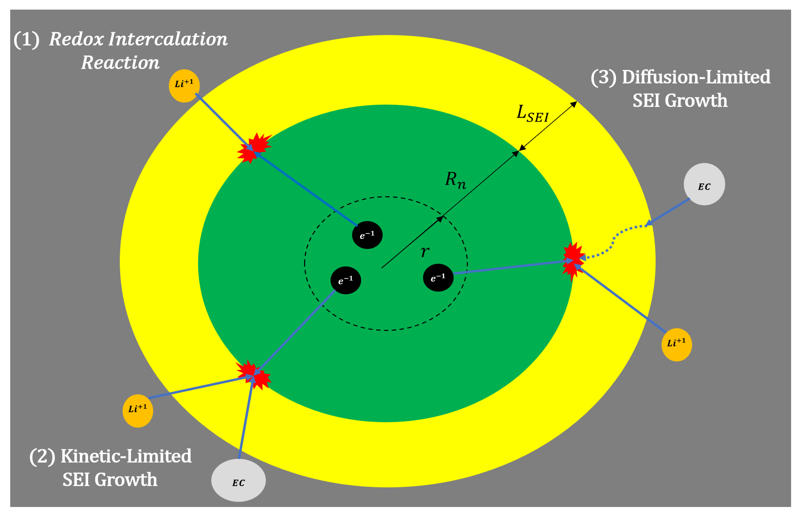
2.2. SEI Growth Models
2.2.1. Kinetic-Limited Reaction Model
2.2.2. Diffusion-Limited Reaction Model
2.2.3. SEI Thickness, Resistance, and Capacity Lost
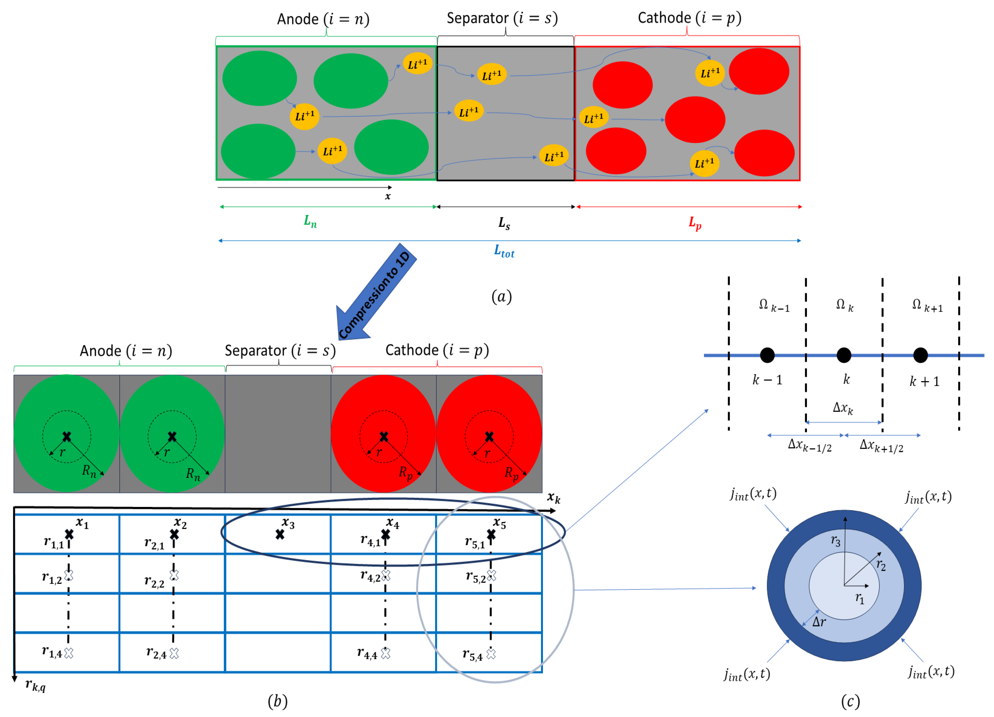
3. Model Discretisation
3.1. Mesh Generation
3.1.1. Mesh Generation in x Dimension
3.1.2. Mesh Generation in r Dimension
3.2. Finite Volume Method
3.2.1. PDAE Discretisation in the x Dimension
3.2.2. PDAE Discretisation in the r Dimension
3.3. Spatial Boundary Condition Implementation
3.3.1. Boundaries between Material Domains
3.3.2. Boundaries within a Material Domain
3.3.3. Other Boundary Conditions
3.4. Verlet Integration
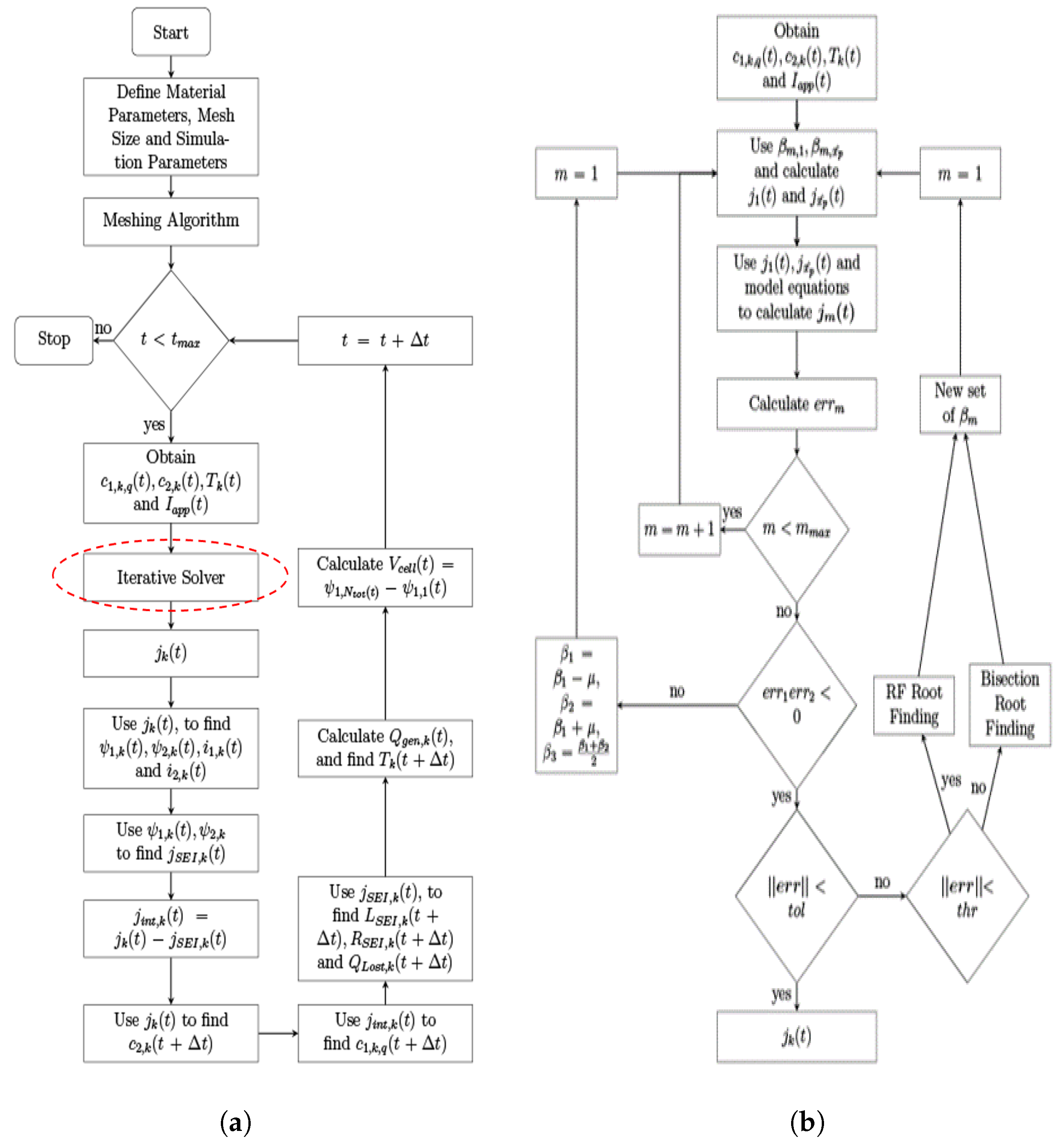
4. Solver Algorithm
4.1. The Iterative Solver
4.1.1. Root Window Searching
4.1.2. Hybrid Root-Finding Algorithm
5. Results and Discussion
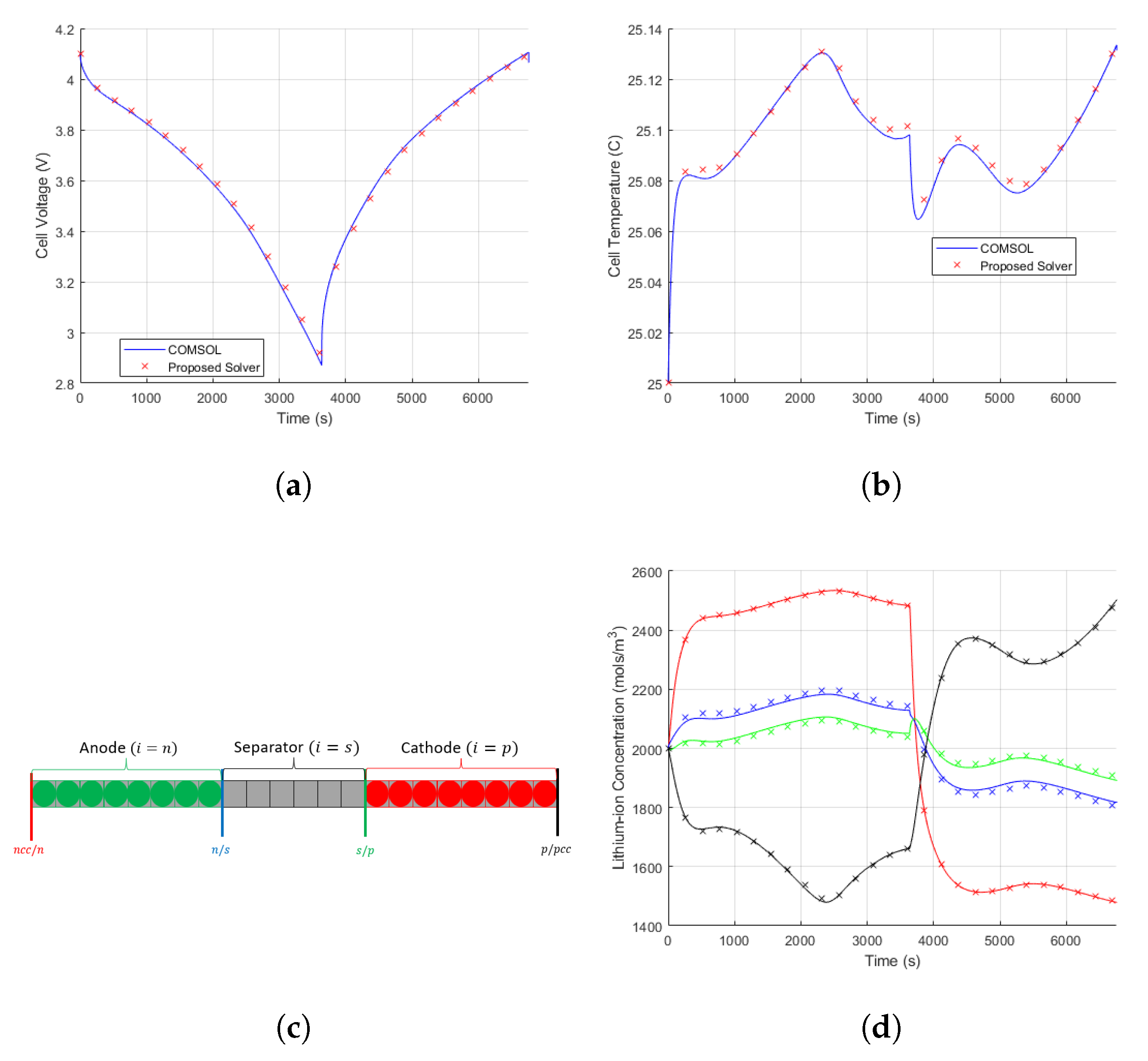
5.1. Single Discharge/Charge Cycle Validation
5.2. Temperature Variation in the P2D Model
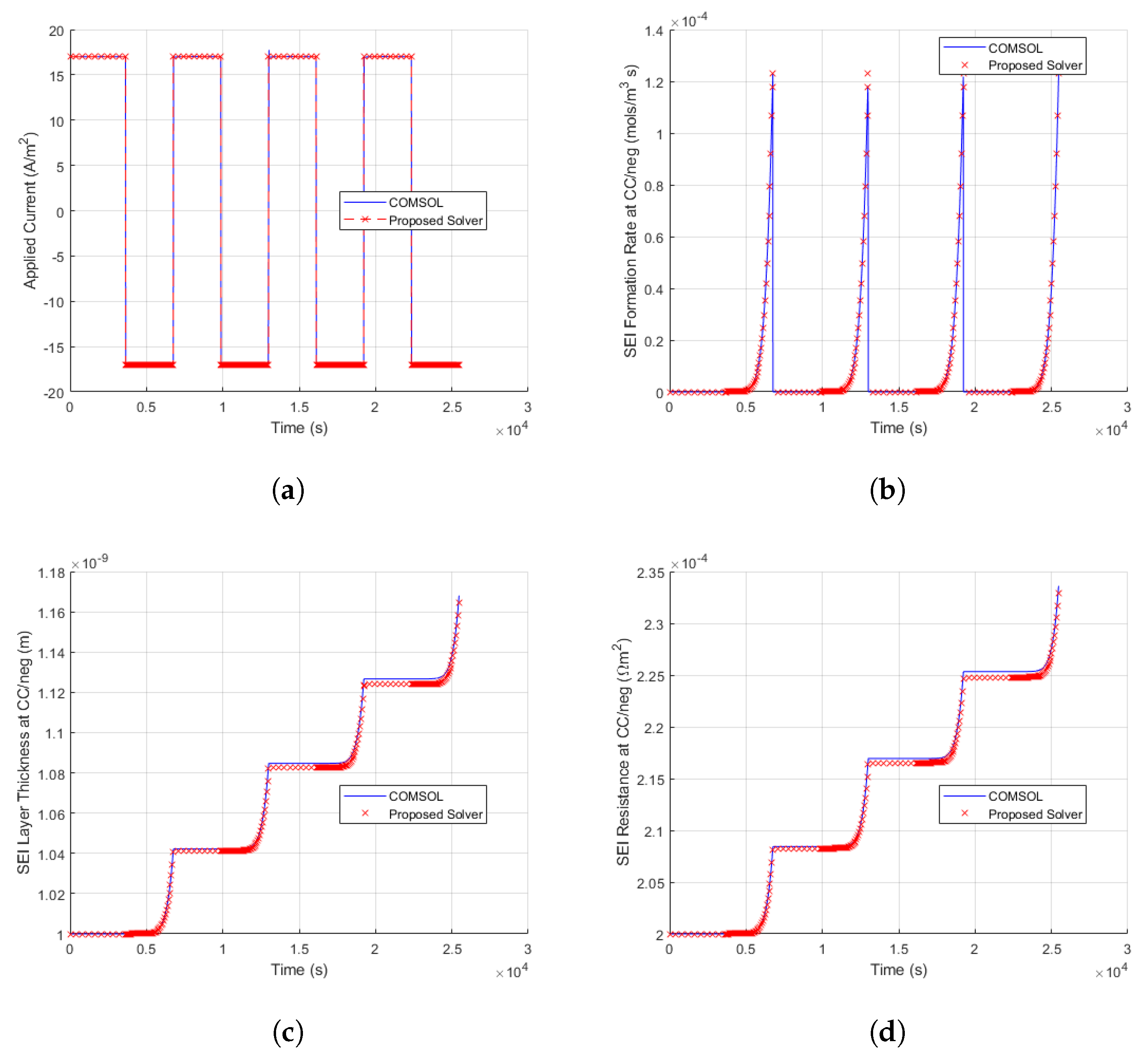
5.3. Validation of Kinetic SEI Growth Model
5.4. Multi-C-Rate Discharge Validation
5.5. Drive Cycle Validation
5.6. Solver Performance
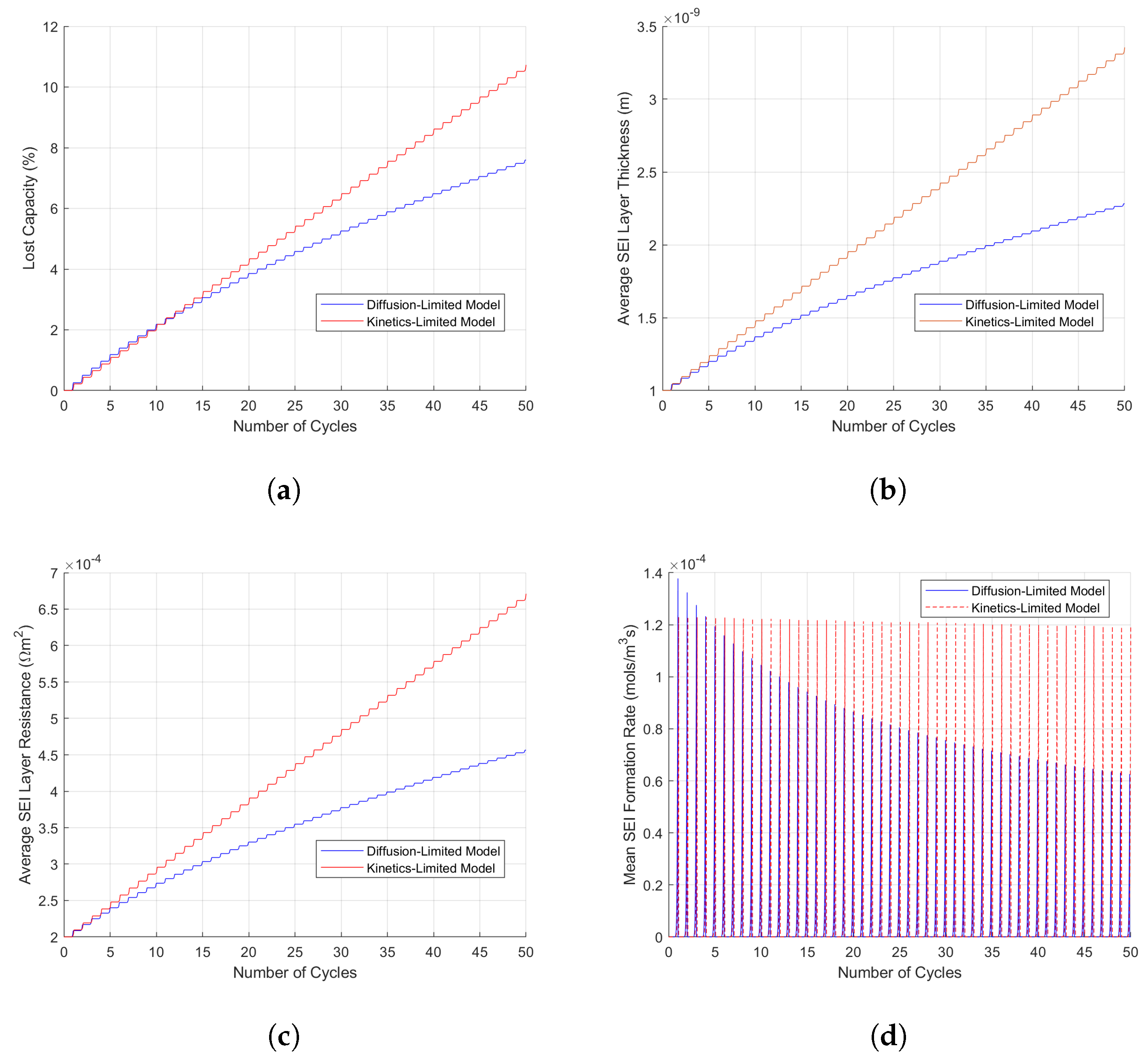
5.7. SEI Growth Model Comparison
6. Conclusions
Author Contributions
Funding
Data Availability Statement
Conflicts of Interest
Appendix A
References
- Grey, C.P.; Hall, D.S. Prospects for lithium-ion batteries and beyond—A 2030 vision. Nat. Commun. 2020, 11, 6279. [Google Scholar] [CrossRef] [PubMed]
- Lu, L.; Han, X.; Li, J.; Hua, J.; Ouyang, M. A review on the key issues for lithium-ion battery management in electric vehicles. J. Power Sources 2013, 226, 272–288. [Google Scholar] [CrossRef]
- Abada, S.; Marlair, G.; Lecocq, A.; Petit, M.; Sauvant-Moynot, V.; Huet, F. Safety focused modeling of lithium-ion batteries: A review. J. Power Sources 2016, 306, 178–192. [Google Scholar] [CrossRef]
- Liu, W.; Placke, T.; Chau, K.T. Overview of batteries and battery management for electric vehicles. Energy Rep. 2022, 8, 4058–4084. [Google Scholar] [CrossRef]
- Plett, G.L. Battery Management Systems, Volume I: Battery Modeling; Artech House: Minto, Australia, 2015; Volume 1. [Google Scholar]
- Ramadesigan, V.; Northrop, P.W.C.; De, S.; Santhanagopalan, S.; Braatz, R.D.; Subramanian, V.R. Modeling and Simulation of Lithium-Ion Batteries from a Systems Engineering Perspective. J. Electrochem. Soc. 2012, 159, R31–R45. [Google Scholar] [CrossRef]
- Zhang, C.; Li, K.; McLoone, S.; Yang, Z. Battery modelling methods for electric vehicles—A review. In Proceedings of the 2014 European Control Conference, ECC 2014, Strasbourg, France, 24–27 June 2014; pp. 2673–2678. [Google Scholar] [CrossRef]
- Liaw, B.Y.; Nagasubramanian, G.; Jungst, R.G.; Doughty, D.H. Modeling of lithium ion cells—A simple equivalent-circuit model approach. Solid State Ionics 2004, 175, 835–839. [Google Scholar] [CrossRef]
- Seaman, A.; Dao, T.S.; Mcphee, J. A survey of mathematics-based equivalent-circuit and electrochemical battery models for hybrid and electric vehicle simulation. J. Power Sources 2014, 256, 410–423. [Google Scholar] [CrossRef]
- Jokar, A.; Rajabloo, B.; Désilets, M.; Lacroix, M. Review of simplified Pseudo-two-Dimensional models of lithium-ion batteries. J. Power Sources 2016, 327, 44–55. [Google Scholar] [CrossRef]
- Doyle, M.; Fuller, T.F.; Newman, J. Modeling of Galvanostatic Charge and Discharge of the Lithium/Polymer/Insertion Cell. J. Electrochem. Soc. 1993, 140, 1526–1533. [Google Scholar] [CrossRef]
- Fuller, T.F.; Doyle, M.; Newman, J. Simulation and Optimization of the Dual Lithium Ion Insertion Cell. J. Electrochem. Soc. 1994, 141, 1. [Google Scholar] [CrossRef]
- Rao, L.; Newman, J. Heat-Generation Rate and General Energy Balance for Insertion Battery Systems. J. Electrochem. Soc. 1997, 144, 2697–2704. [Google Scholar] [CrossRef]
- Farag, M.; Sweity, H.; Fleckenstein, M.; Habibi, S. Combined electrochemical, heat generation, and thermal model for large prismatic lithium-ion batteries in real-time applications. J. Power Sources 2017, 360, 618–633. [Google Scholar] [CrossRef]
- Ramadass, P.; Haran, B.; Gomadam, P.M.; White, R.; Popov, B.N. Development of First Principles Capacity Fade Model for Li-Ion Cells. J. Electrochem. Soc. 2004, 151, A196. [Google Scholar] [CrossRef]
- Pinson, M.B.; Bazant, M.Z. Theory of SEI Formation in Rechargeable Batteries: Capacity Fade, Accelerated Aging and Lifetime Prediction. J. Electrochem. Soc. 2012, 160, A243–A250. [Google Scholar] [CrossRef]
- Ramos, A.M. On the well-posedness of a mathematical model for Lithium-ion batteries. Appl. Math. Model. 2015, 40, 115–125. [Google Scholar] [CrossRef]
- Bermejo, R. Numerical analysis of a finite element formulation of the P2D model for Lithium-ion cells. Numer. Math. 2021, 149, 463–505. [Google Scholar] [CrossRef]
- Zhang, D.; Popov, B.N.; White, R.E. Modeling Lithium Intercalation of a Single Spinel Particle under Potentiodynamic Control. J. Electrochem. Soc. 2000, 147, 831. [Google Scholar] [CrossRef]
- Luo, W.; Lyu, C.; Wang, L.; Zhang, L. An approximate solution for electrolyte concentration distribution in physics-based lithium-ion cell models. Microelectron. Reliab. 2013, 53, 797–804. [Google Scholar] [CrossRef]
- Kim, G.H.; Smith, K.; Lawrence-Simon, J.; Yang, C. Efficient and Extensible Quasi-Explicit Modular Nonlinear Multiscale Battery Model: GH-MSMD. J. Electrochem. Soc. 2017, 164, A1076–A1088. [Google Scholar] [CrossRef]
- Ma, Y.; Yin, M.; Ying, Z.; Chen, H. Establishment and simulation of an electrode averaged model for a lithium-ion battery based on kinetic reactions. RSC Adv. 2016, 6, 25435–25443. [Google Scholar] [CrossRef]
- Perez, H.E.; Hu, X.; Moura, S.J. Optimal charging of batteries via a single particle model with electrolyte and thermal dynamics. In Proceedings of the 2016 American Control Conference (ACC), Boston, MA, USA, 6–8 July 2016; pp. 4000–4005. [Google Scholar] [CrossRef]
- Yin, X.; Zhang, D. batP2dFoam: An Efficient Segregated Solver for the Pseudo-2-Dimensional (P2D) Model of Li-Ion Batteries. J. Electrochem. Soc. 2023, 170, 030521. [Google Scholar] [CrossRef]
- Chen, Q.; Chen, X.S.; Li, Z. A fast numerical method with non-iterative source term for pseudo-two-dimension lithium-ion battery model. J. Power Sources 2023, 577, 233258. [Google Scholar] [CrossRef]
- Ai, W.; Liu, Y. Improving the convergence rate of Newman’s battery model using 2nd order finite element method. J. Energy Storage 2023, 67, 107512. [Google Scholar] [CrossRef]
- Chayambuka, K.; Mulder, G.; Danilov, D.L.; Notten, P.H. Physics-based modeling of sodium-ion batteries part II. Model and validation. Electrochim. Acta 2022, 404, 139764. [Google Scholar] [CrossRef]
- Jiang, Y.; Zhang, L.; Offer, G.; Wang, H. A user-friendly lithium battery simulator based on open-source CFD. Digit. Chem. Eng. 2022, 5, 100055. [Google Scholar] [CrossRef]
- Han, S.; Tang, Y.; Rahimian, S.K. A numerically efficient method of solving the full-order pseudo-2-dimensional (P2D) Li-ion cell model. J. Power Sources 2021, 490, 229571. [Google Scholar] [CrossRef]
- Geng, Z.; Wang, S.; Lacey, M.J.; Brandell, D.; Thiringer, T. Bridging physics-based and equivalent circuit models for lithium-ion batteries. Electrochim. Acta 2021, 372, 137829. [Google Scholar] [CrossRef]
- Han, R.; Macdonald, C.; Wetton, B. A fast solver for the pseudo-two-dimensional model of lithium-ion batteries. arXiv 2021, arXiv:2111.09251. [Google Scholar]
- Noor, A.S.; Kadhim, A.H.; Ali, M.A.; Zülke, A.; Korotkin, I. DandeLiion v1: An Extremely Fast Solver for the Newman Model of Lithium-Ion Battery (Dis)charge. J. Electrochem. Soc. 2021, 168, 060544. [Google Scholar] [CrossRef]
- Lee, S.B.; Onori, S. A Robust and Sleek Electrochemical Battery Model Implementation: A MATLAB® Framework. J. Electrochem. Soc. 2021, 168, 090527. [Google Scholar] [CrossRef]
- Esfahanian, V.; Chaychizadeh, F.; Dehghandorost, H.; Shokouhmand, H. An Efficient Thermal-Electrochemical Simulation of Lithium-Ion Battery Using Proper Mathematical-Physical CFD Schemes. J. Electrochem. Soc. 2019, 166, A1520–A1534. [Google Scholar] [CrossRef]
- Guo, M.; Jin, X.; White, R.E. Nonlinear State-Variable Method for Solving Physics-Based Li-Ion Cell Model with High-Frequency Inputs. J. Electrochem. Soc. 2017, 164, E3001–E3015. [Google Scholar] [CrossRef]
- Torchio, M.; Magni, L.; Gopaluni, R.B.; Braatz, R.D.; Raimondo, D.M. LIONSIMBA: A Matlab Framework Based on a Finite Volume Model Suitable for Li-Ion Battery Design, Simulation, and Control. J. Electrochem. Soc. 2016, 163, A1192–A1205. [Google Scholar] [CrossRef]
- Tulsyan, A.; Tsai, Y.; Gopaluni, R.B.; Braatz, R.D. State-of-charge estimation in lithium-ion batteries: A particle filter approach. J. Power Sources 2016, 331, 208–223. [Google Scholar] [CrossRef]
- Wickramanayake, T.; Javadipour, M.; Mehran, K. A Novel Root-Finding Algorithm to Solve the Pseudo-2D Model of a Lithium-ion Battery. In Proceedings of the 2023 IEEE International Conference on Electrical Systems for Aircraft, Railway, Ship Propulsion and Road Vehicles and International Transportation Electrification Conference, ESARS-ITEC 2023, Venice, Italy, 29–31 March 2023. [Google Scholar] [CrossRef]
- Mai, W.; Colclasure, A.; Smith, K. A Reformulation of the Pseudo2D Battery Model Coupling Large Electrochemical-Mechanical Deformations at Particle and Electrode Levels. J. Electrochem. Soc. 2019, 166, A1330–A1339. [Google Scholar] [CrossRef]
- Liu, L.; Park, J.; Lin, X.; Sastry, A.M.; Lu, W. A thermal-electrochemical model that gives spatial-dependent growth of solid electrolyte interphase in a Li-ion battery. J. Power Sources 2014, 268, 482–490. [Google Scholar] [CrossRef]
- Birkl, C.R.; Roberts, M.R.; McTurk, E.; Bruce, P.G.; Howey, D.A. Degradation diagnostics for lithium ion cells. J. Power Sources 2017, 341, 373–386. [Google Scholar] [CrossRef]
- Edge, J.S.; O’Kane, S.; Prosser, R.; Kirkaldy, N.D.; Patel, A.N.; Hales, A.; Ghosh, A.; Ai, W.; Chen, J.; Yang, J.; et al. Lithium ion battery degradation: What you need to know. Phys. Chem. Chem. Phys. 2021, 23, 8200–8221. [Google Scholar] [CrossRef]
- O’Kane, S.E.; Ai, W.; Madabattula, G.; Alonso-Alvarez, D.; Timms, R.; Sulzer, V.; Edge, J.S.; Wu, B.; Offer, G.J.; Marinescu, M. Lithium-ion battery degradation: How to model it. Phys. Chem. Chem. Phys. 2022, 24, 7909–7922. [Google Scholar] [CrossRef] [PubMed]
- Reniers, J.M.; Mulder, G.; Howey, D.A. Review and Performance Comparison of Mechanical-Chemical Degradation Models for Lithium-Ion Batteries. J. Electrochem. Soc. 2019, 166, A3189–A3200. [Google Scholar] [CrossRef]
- Lamorgese, A.; Mauri, R.; Tellini, B. Electrochemical-thermal P2D aging model of a LiCoO2/graphite cell: Capacity fade simulations. J. Energy Storage 2018, 20, 289–297. [Google Scholar] [CrossRef]
- Awarke, A.; Pischinger, S.; Ogrzewalla, J. Pseudo 3D Modeling and Analysis of the SEI Growth Distribution in Large Format Li-Ion Polymer Pouch Cells. J. Electrochem. Soc. 2013, 160, A172–A181. [Google Scholar] [CrossRef]
- Ashwin, T.R.; Chung, Y.M.; Wang, J. Capacity fade modelling of lithium-ion battery under cyclic loading conditions. J. Power Sources 2016, 328, 586–598. [Google Scholar] [CrossRef]
- Kamyab, N.; Weidner, J.W.; White, R.E. Mixed Mode Growth Model for the Solid Electrolyte Interface (SEI). J. Electrochem. Soc. 2019, 166, A334–A341. [Google Scholar] [CrossRef]
- Das, S.; Attia, P.M.; Chueh, W.C.; Bazant, M.Z. Electrochemical Kinetics of SEI Growth on Carbon Black: Part II. Modeling. J. Electrochem. Soc. 2019, 166, E107–E118. [Google Scholar] [CrossRef]
- Cheng, H.; Sun, Q.; Li, L.; Zou, Y.; Wang, Y.; Cai, T.; Zhao, F.; Liu, G.; Ma, Z.; Wahyudi, W.; et al. Emerging Era of Electrolyte Solvation Structure and Interfacial Model in Batteries. ACS Energy Lett. 2022, 7, 490–513. [Google Scholar] [CrossRef]
- Botte, G.G.; Ritter, J.A.; White, R.E. Comparison of finite difference and control volume methods for solving differential equations. Comput. Chem. Eng. 2000, 24, 2633–2654. [Google Scholar] [CrossRef]
- Kong, X.R.; Wetton, B.; Gopaluni, B. Assessment of Simplifications to a Pseudo–2D Electrochemical Model of Li-ion Batteries. IFAC-PapersOnLine 2019, 52, 946–951. [Google Scholar] [CrossRef]
- Zwillinger, D. CRC Standard Mathematical Tables and Formulae; Chapman and Hall/CRC: Boca Raton, FL, USA, 2003; p. 910. [Google Scholar]
- Butcher, J.C. Numerical Methods for Ordinary Differential Equations; John Wiley & Sons: Hoboken, NJ, USA, 2016; pp. 1–513. [Google Scholar] [CrossRef]
- Hairer, E.; Lubich, C.; Wanner, G. Geometric numerical integration illustrated by the Störmer-Verlet method. Acta Numer. 2000, 12, 399–450. [Google Scholar] [CrossRef]
- Hosseinzadeh, E.; Marco, J.; Jennings, P. Electrochemical-Thermal Modelling and Optimisation of Lithium-Ion Battery Design Parameters Using Analysis of Variance. Energies 2017, 10, 1278. [Google Scholar] [CrossRef]
- Dahlquist, G.; Bjorck, A. Numerical Methods; Anderson, N., Translator; Prentice-Hall Series in Automatic Computation; Prentice-Hall: Englewood Cliffs, NJ, USA, 1974. [Google Scholar]
- Chalise, D.; Lu, W.; Srinivasan, V.; Prasher, R. Heat of Mixing During Fast Charge/Discharge of a Li-Ion Cell: A Study on NMC523 Cathode. J. Electrochem. Soc. 2020, 167, 090560. [Google Scholar] [CrossRef]
- Mayer, S. Electric Vehicle Dynamic-Stress-Test Cycling Performance of Lithium-Ion Cells; Lawrence Livermore National Lab. (LLNL): Livermore, CA, USA, 1994. [Google Scholar] [CrossRef]
- COMSOL Inc. 1D Lithium-Ion Battery Drive-Cycle Monitoring; COMSOL: Stockholm, Sweden, 2023. [Google Scholar]
- Agubra, V.A.; Fergus, J.W. The formation and stability of the solid electrolyte interface on the graphite anode. J. Power Sources 2014, 268, 153–162. [Google Scholar] [CrossRef]


| Parameters Solved | ||||
|---|---|---|---|---|
| Paper | Discretisation Method | Isothermal P2D | Temperature Modelling | Ageing Model |
| Yin et al. (2023) [24] | FVM | × | - | - |
| Chen et al. (2023) [25] | FDM | × | - | - |
| Ai et al. (2023) [26] | FEM | × | - | - |
| Chayambuka et al. (2022) [27] | FDM + FVM at boundaries | × | - | - |
| Jiang et al. (2022) [28] | FVM | × | - | - |
| Han et al. (2021) [29] | FVM | × | ROM | - |
| Geng et al. (2021) [30] | FDM | × | - | - |
| Han et al. (2021) [31] | FDM | × | FOM | - |
| Noor et al. (2021) [32] | FEM | × | - | - |
| Lee et al. (2021) [33] | FDM | × | - | - |
| Esfahanian et al. (2019) [34] | FVM | × | FOM | - |
| Guo et al. (2017) [35] | Nonlinear State-Variable Method | × | - | - |
| Torchio et al. (2016) [36] | FVM | × | FOM | - |
| Tulsyan et al. (2016) [37] | State-Space Method | × | - | - |
| Doyle et al. (1993) [11] | FDM | × | - | - |
| Proposed solver | FVM | × | FOM | × |
| Differential Equations | Boundary Conditions | |
|---|---|---|
| (P1) Solid-Phase Diffusion | ||
| , | (1) | |
| (P2) Electrolyte-Phase Diffusion | ||
| (2) | ||
| (P3) Ohm’s Law in Solid Phase | ||
| , | (3) | |
| (P4) Ohm’s Law in Electrolyte Phase | ||
| (4) | ||
| (P5) Kirchhoff’s Current Law | ||
| (5) | ||
| for | (6) | |
| (7) | ||
| (P6) Redox Reaction Exchange Flux | ||
| (8) | ||
| (9) | ||
| for | (10) | |
| (P7) Thermal Energy Balance | ||
| (11) |
| Open-Circuit Potentials | |
| (12) | |
| (13) | |
| Stoichiometry | |
| (14) | |
| (15) | |
| Open-Circuit Potential Function | |
| 1 | (16) |
| 1 | |
| (17) | |
| Entropy Change | |
| (18) | |
| (19) | |
| Electrolyte Conductivity | |
| 1 | (20) |
| (21) | |
| Particle Surface-Area-to-Volume Ratio | |
| (22) | |
| Bruggeman Parameter Corrections | |
| (23) | |
| (24) | |
| Arrhenius Relationships | |
| (25) | |
| (26) | |
| Heat Generation | |
| (27) | |
| (28) | |
| (29) | |
| (30) |
| Boundary Condition | Grid Position | |
|---|---|---|
| (P1) Solid-Phase Diffusion | ||
| , , | (65) | |
| , , | (66) | |
| (P2) Electrolyte-Phase Diffusion | ||
| (67) | ||
| (68) | ||
| (P3) Ohm’s Law in Solid Phase | ||
| (69) | ||
| (70) | ||
| (P4) Ohm’s Law in Electrolyte Phase | ||
| (71) | ||
| (72) | ||
| (P5) Kirchhoff’s Current Law | ||
| (73) | ||
| (74) | ||
| (75) | ||
| (P6) Redox Reaction Exchange Flux | ||
| (76) | ||
| (P7) Thermal Energy Balance | ||
| (77) | ||
| (78) |
| Parameter | Description | Units | Anode | Separator | Cathode |
|---|---|---|---|---|---|
| 2 | Initial State of Charge | - | 0.58 | - | 0.19 |
| 1 | Maximum Solid-Phase Lithium Concentration | mols/m3 | 26,390 | - | 22,860 |
| 2 | Initial Solid-Phase Lithium Concentration | mols/m3 | - | ||
| 1 | Initial Electrolyte-Phase Lithium-ion Concentration | mols/m3 | 2000 | 2000 | 2000 |
| 1 | Solid-Phase Lithium Diffusivity | m2/s | 3.9 | - | 1 |
| 1 | Electrolyte-Phase Lithium-ion Diffusivity | m2/s | 7.5 | 7.5 | 7.5 |
| 1 | Solid-Phase Electrical Conductivity | S/m | 100.0 | - | 3.8 |
| 1 | Thickness of Domain | m | 100 | 52 | 183 |
| 1 | Electrode Particle Radius | m | 12.5 | - | 8.5 |
| 1 | Electrode Volume Fraction | - | 0.471 | - | 0.2970 |
| 1 | Porosity | - | 0.3570 | 1.0 | 0.4440 |
| 1 | Bruggeman Coefficient | - | 1.5 | 1.5 | 1.5 |
| 2 | Intercalation Reaction Rate Constant | m2.5/(mol0.5s) | 2 | - | 2 |
| 1 | Intercalation Reaction Transfer Coefficient | - | 0.5 | - | 0.5 |
| 1 | Lithium-ion Transference Number | - | 0.3630 | 0.3630 | 0.3630 |
| F | Faraday Constant | Col/mol | 96,487 | 96,487 | 96,487 |
| R | Ideal Gas Constant | J/(mol K) | 8.314 | 8.314 | 8.314 |
| 1 | Domain Density | kg/m3 | 2500 | 1200 | 1500 |
| 1 | Domain Specific Heat Capacity | J/(Kg K) | 700 | 700 | 700 |
| 1 | Domain Thermal Conductivity | W/(m K) | 5 | 1 | 5 |
| 1 | Intercalation Reaction Rate Activation Energy | J/mol | 30,000 | - | 30,000 |
| 1 | Solid-Phase Diffusivity Activation Energy | J/mol | 4000 | - | 20,000 |
| 1 | Heat Exchange Coefficient | W/(m2 K) | 5 | - | 5 |
| 1 | Ambient Temperature | C | 25.15 | - | 25.15 |
| 1 | Initial Cell Temperature | C | 25.15 | 25.15 | 25.15 |
| 1 | Initial SEI Thickness | m | 1 | - | - |
| 2 | Initial SEI Resistance | m2 | 2 | - | - |
| 1 | SEI Lithium Conductivity | Sm | 5 | - | - |
| 1 | SEI Molar Mass | kg/mol | 0.1620 | - | - |
| 1 | SEI Density | kg/m3 | 1690 | - | - |
| 1 | SEI Reaction Transfer Coefficient | - | 0.5 | - | - |
| 2 | Number of Electrons Involved in SEI Reaction | - | 2 | - | - |
| 1 | Open-Circuit Potential of SEI Growth | V | 0 | - | - |
| 2 | Kinetic-Limited SEI Exchange Current | A/m2 | 8.8 | - | - |
| 2 | SEI Reaction Rate Coefficient | m/s2 | 2 | - | - |
| 2 | Diffusivity of Electrolyte Solvent in SEI | m2/s | 3.5 | - | - |
| 1 | Concentration of Solvent in Bulk Electrolyte | mols/m3 | 4541 | - | - |
| 2 | Porosity of SEI Layer | - | 0.03 | - | - |
| Percentage Errors | 0.44% | 0.43% | 2.82% | 2.81% | <0.01% |
| 0.25C | 0.5C | 1.0C | 2.0C | 5.0C | 10.0C | |
|---|---|---|---|---|---|---|
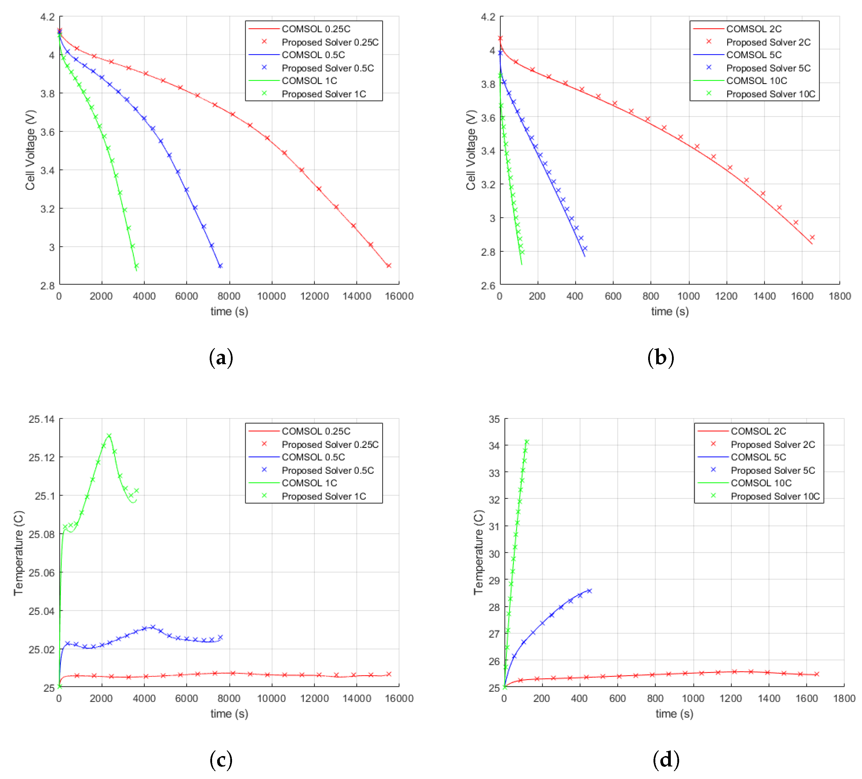
| 0.13% | 0.25% | 0.44% | 0.71% | 0.98% | 1.7% | |
| <0.01% | <0.01% | <0.01% | 0.02% | 0.15% | 0.3% |
| Parameters | Dynamic Stress Test | COMSOL Dynamic Drive Cycle |
|---|---|---|
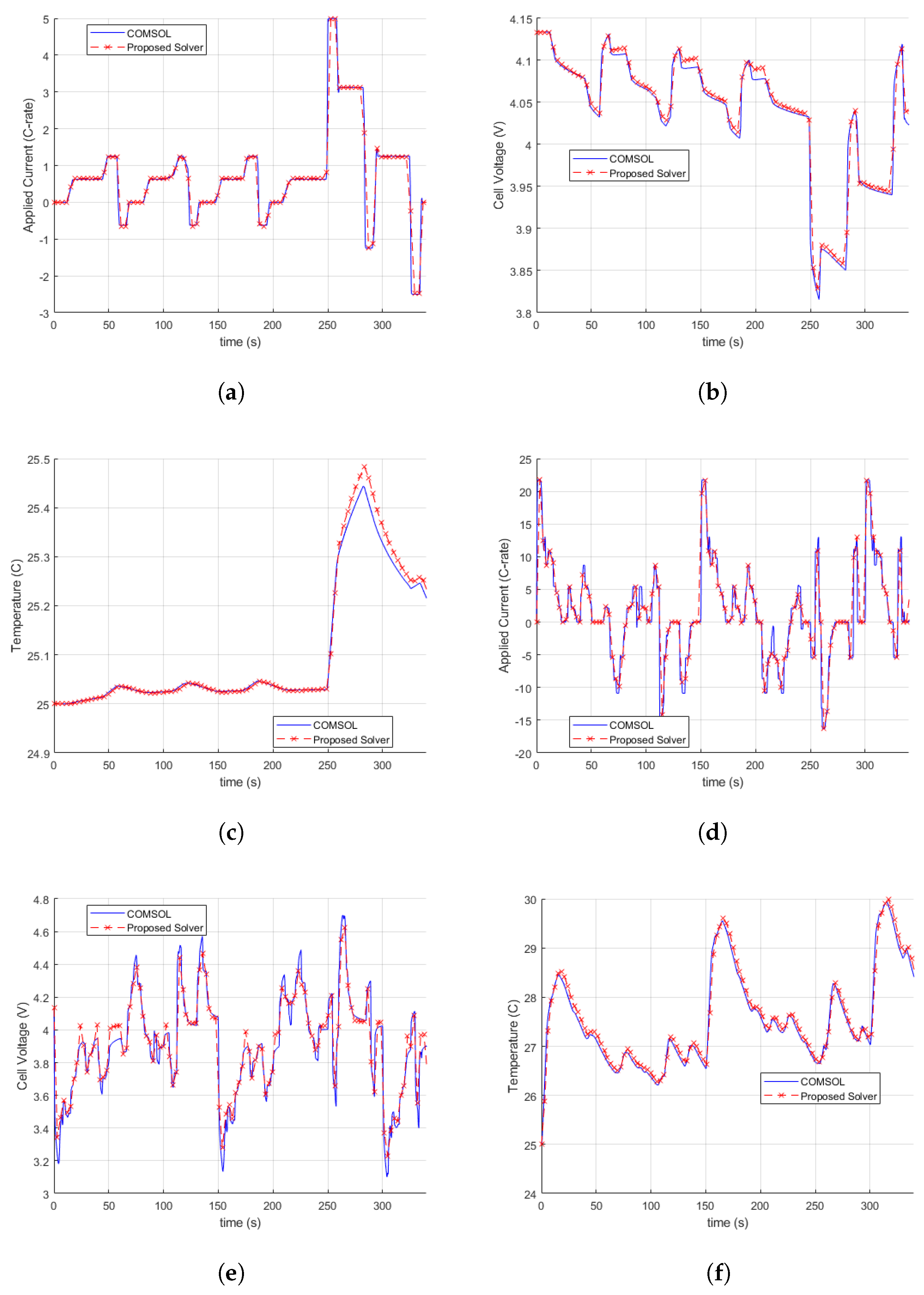
| 0.4% | 1% | |
| 0.05% | 0.02% |
| Number of Elements in x | ||||||||||
|---|---|---|---|---|---|---|---|---|---|---|
| Solver | Discretisation Method | 10 | 20 | 30 | 40 | 50 | 60 | 100 | 200 | 300 |
| 1 Chen et al. [25] | FDM (ROM) | - | - | - | - | - | 10.7 s | * 12.98 s | * 20.04 s | 34.1 s |
| 1 Geng et al. [30] | FDM (ROM) | - | - | - | - | - | 8 s | - | - | - |
| 1 R.Han et al. [31] | FDM | 4.09 s | 4.24 s | 3.98 s | 4.15 s | 4.49 s | - | - | - | - |
| 1 Torchio et al. [31,36] | FVM | 7.46 s | 9.85 s | 15.48 s | 26.80 s | 54.60 s | - | - | - | - |
| 1 Lee et al. [33] | FDM | * 1.28 s | * 2.1 s | - | - | 40.25 s | - | * 50.8 s | - | - |
| 1 Doyle et al. [11,31] | FDM | 28 s | 69 s | 97 s | 137 s | 185 s | - | - | - | - |
| 2 COMSOL | FEM | 9 s | 11 s | 17 s | 23 s | 25 s | 28.4 s | 35 s | - | - |
| 2 Proposed solver | FVM | 1.6 s | 2.2 s | 3.1 s | 3.3 s | 4.3 s | 4.5 s | 7.75 s | 15.3 s | 24.5 s |
Disclaimer/Publisher’s Note: The statements, opinions and data contained in all publications are solely those of the individual author(s) and contributor(s) and not of MDPI and/or the editor(s). MDPI and/or the editor(s) disclaim responsibility for any injury to people or property resulting from any ideas, methods, instructions or products referred to in the content. |
© 2024 by the authors. Licensee MDPI, Basel, Switzerland. This article is an open access article distributed under the terms and conditions of the Creative Commons Attribution (CC BY) license (https://creativecommons.org/licenses/by/4.0/).
Share and Cite
Wickramanayake, T.; Javadipour, M.; Mehran, K. A Novel Solver for an Electrochemical–Thermal Ageing Model of a Lithium-Ion Battery. Batteries 2024, 10, 126. https://doi.org/10.3390/batteries10040126
Wickramanayake T, Javadipour M, Mehran K. A Novel Solver for an Electrochemical–Thermal Ageing Model of a Lithium-Ion Battery. Batteries. 2024; 10(4):126. https://doi.org/10.3390/batteries10040126
Chicago/Turabian StyleWickramanayake, Toshan, Mehrnaz Javadipour, and Kamyar Mehran. 2024. "A Novel Solver for an Electrochemical–Thermal Ageing Model of a Lithium-Ion Battery" Batteries 10, no. 4: 126. https://doi.org/10.3390/batteries10040126
APA StyleWickramanayake, T., Javadipour, M., & Mehran, K. (2024). A Novel Solver for an Electrochemical–Thermal Ageing Model of a Lithium-Ion Battery. Batteries, 10(4), 126. https://doi.org/10.3390/batteries10040126