

State of Charge and State of Health Estimation in Electric Vehicles: Challenges, Approaches and Future Directions


Abstract
1. Introduction
2. SOC Estimation
2.1. Look-Up-Table-Based SOC Estimation
2.2. Direct-Based Method
2.2.1. Ampere-Hour Integral Method
- Dependence on Current Measurements: The precision of current measurements has a significant impact on SOC estimation when utilizing the ampere-hour method. Inaccuracies in SOC estimates may result from current measurement mistakes.
- Error Accumulation: The accuracy of SOC estimates may be considerably impacted over time by inaccuracies in current measurements that accumulate.
- Difficulty in Determining Initial SOC: Accurately determining the initial state of charge (SOC) can be difficult in real-time applications, particularly if the battery is not fully charged or depleted. Precise SOC estimation requires accurate initial SOC.
- Calibration Challenges: Using the Ah technique for SOC estimation can present calibration challenges for both the original SOC and current readings. To take into consideration errors and variances in the system, calibrations are required.
2.2.2. Discharge Test Method
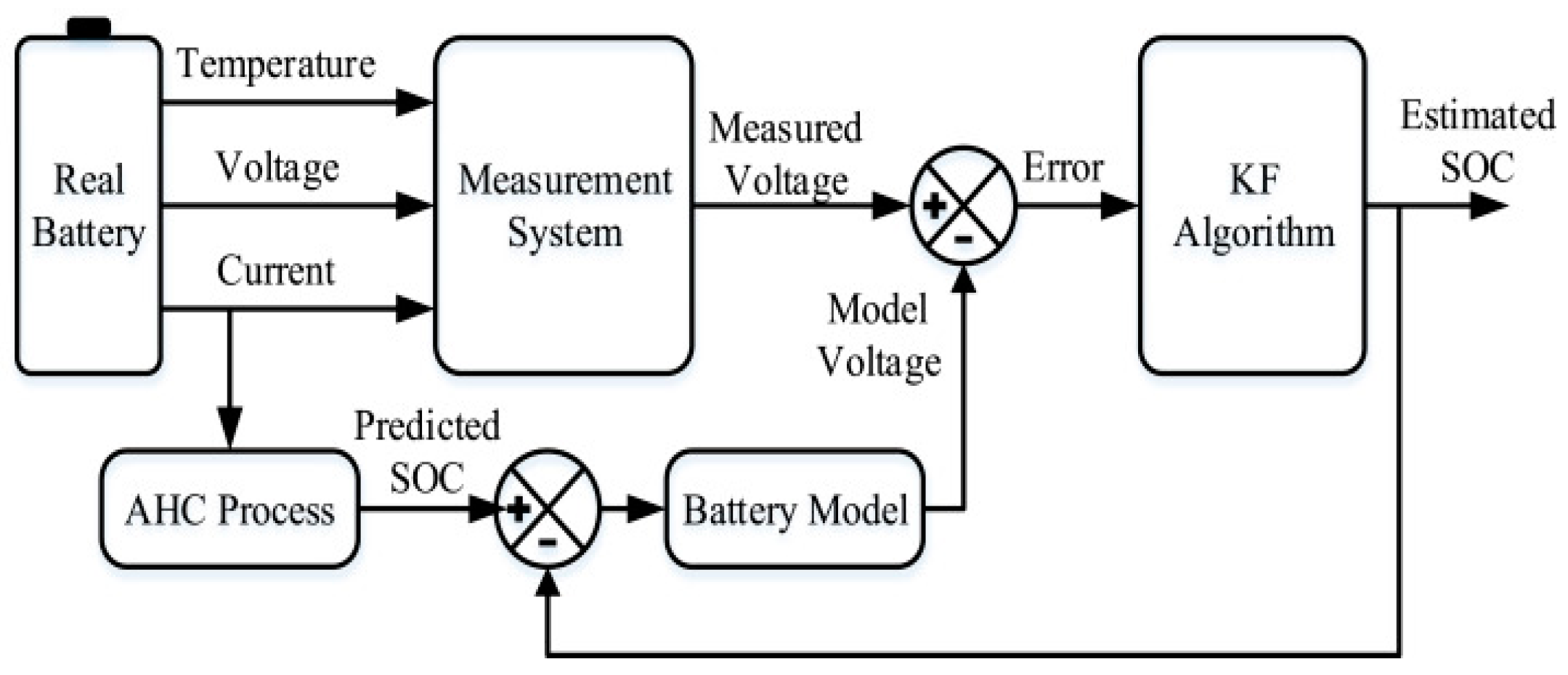
2.3. Model-Based State Estimation
- Linear Kalman filter and variations
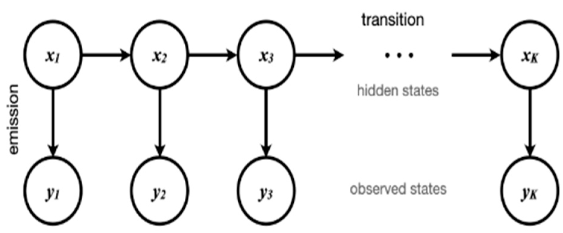
- Sequential Probabilistic Inference.
- Review of probability
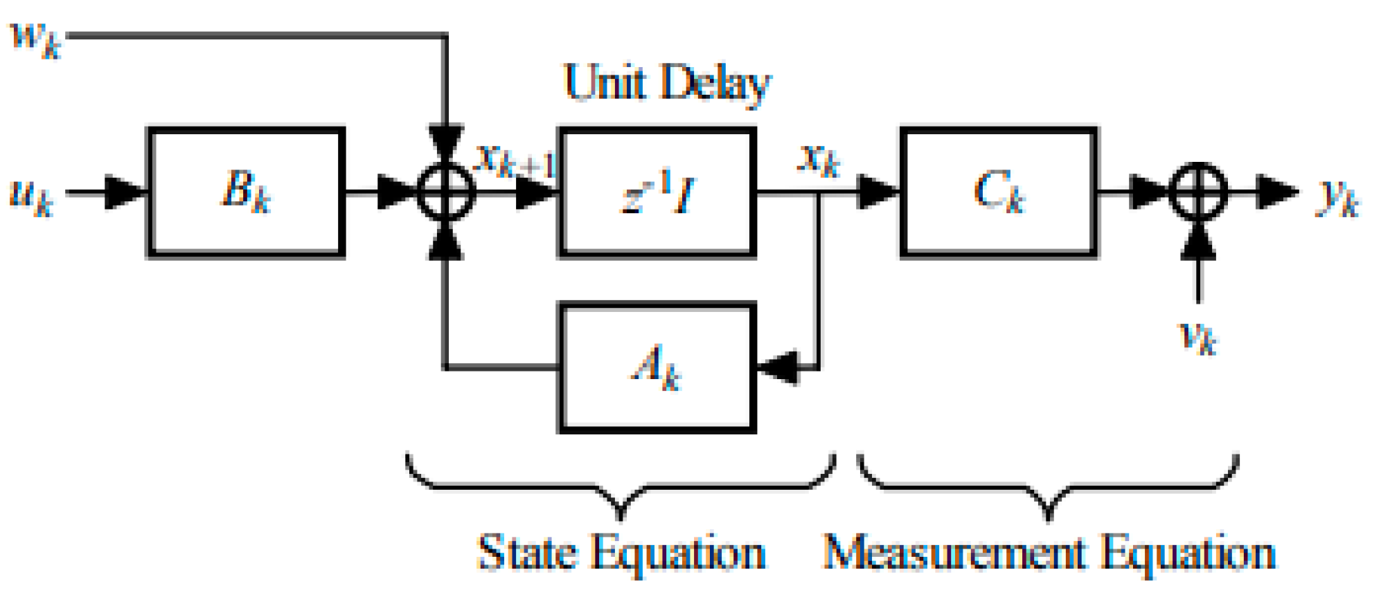
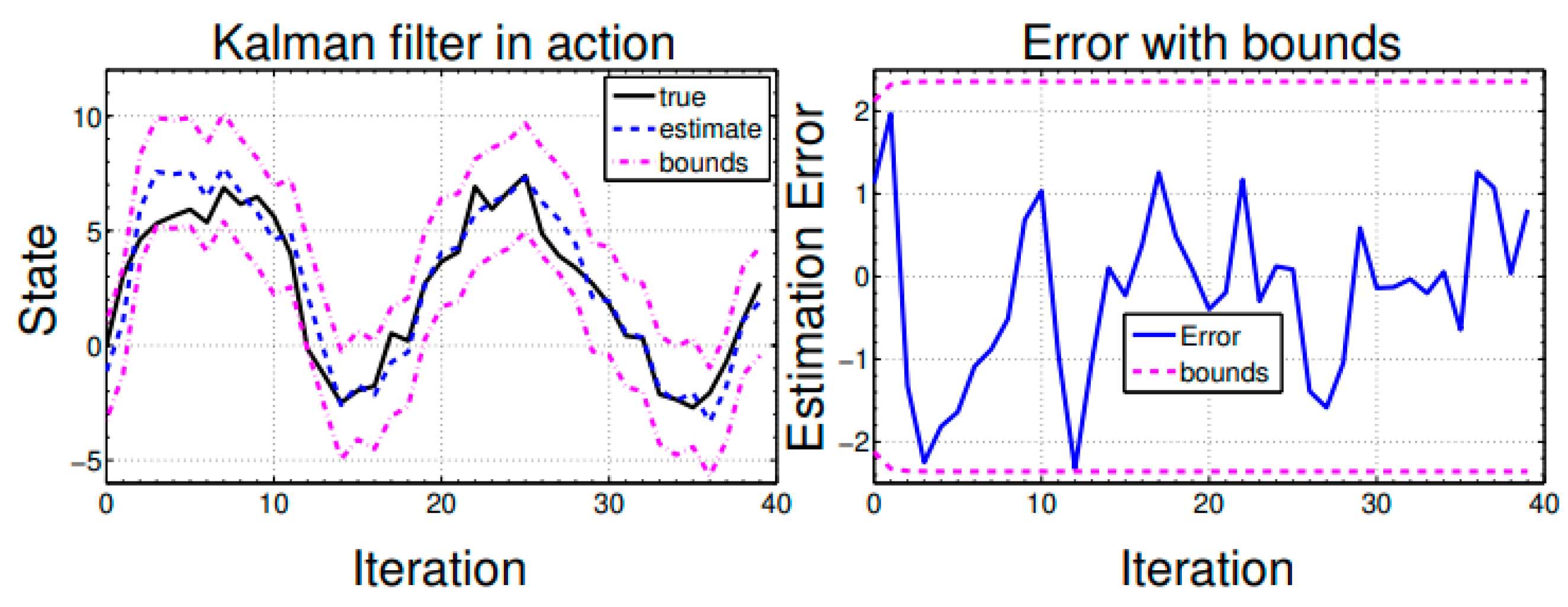
- Linear Kalman Filtering
- Extended Kalman Filtering
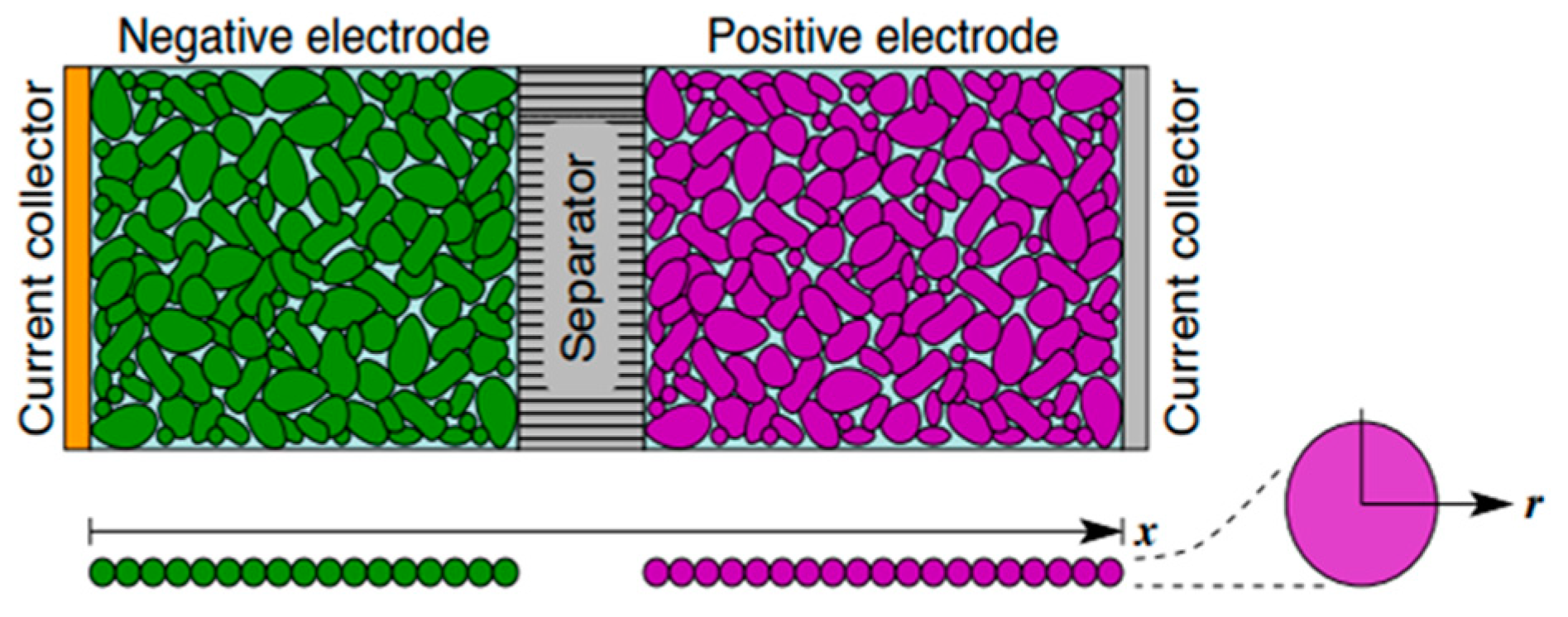
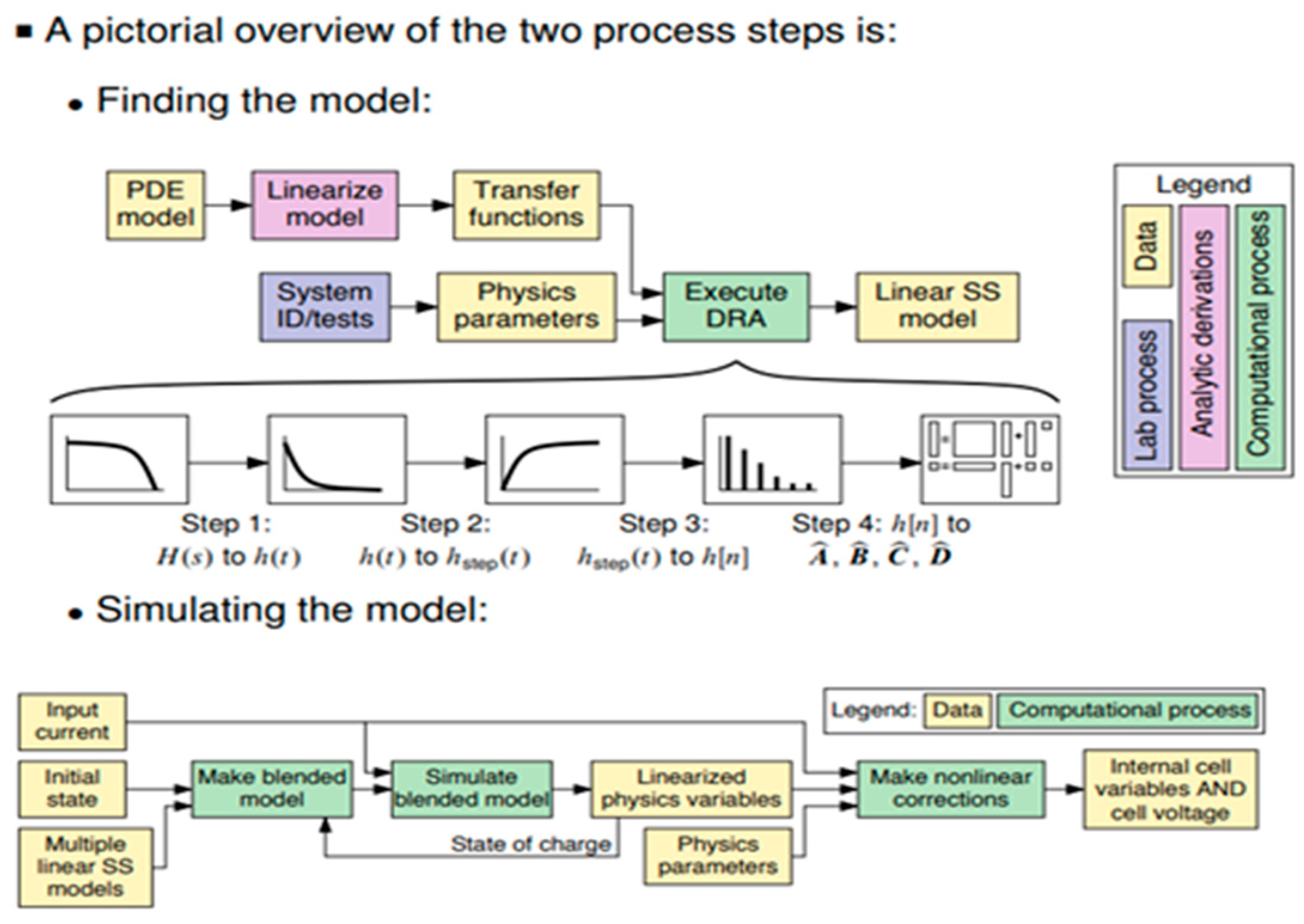
2.3.1. Electrochemical Model
- The presumption was of linear behavior: a Taylor series was used to linearize the nonlinear equations.
- By assuming that the electrolyte concentration Ce(x,t) was not a function of the reaction current j(x,t), transfer functions were built.
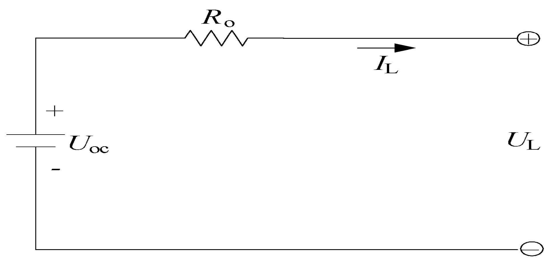
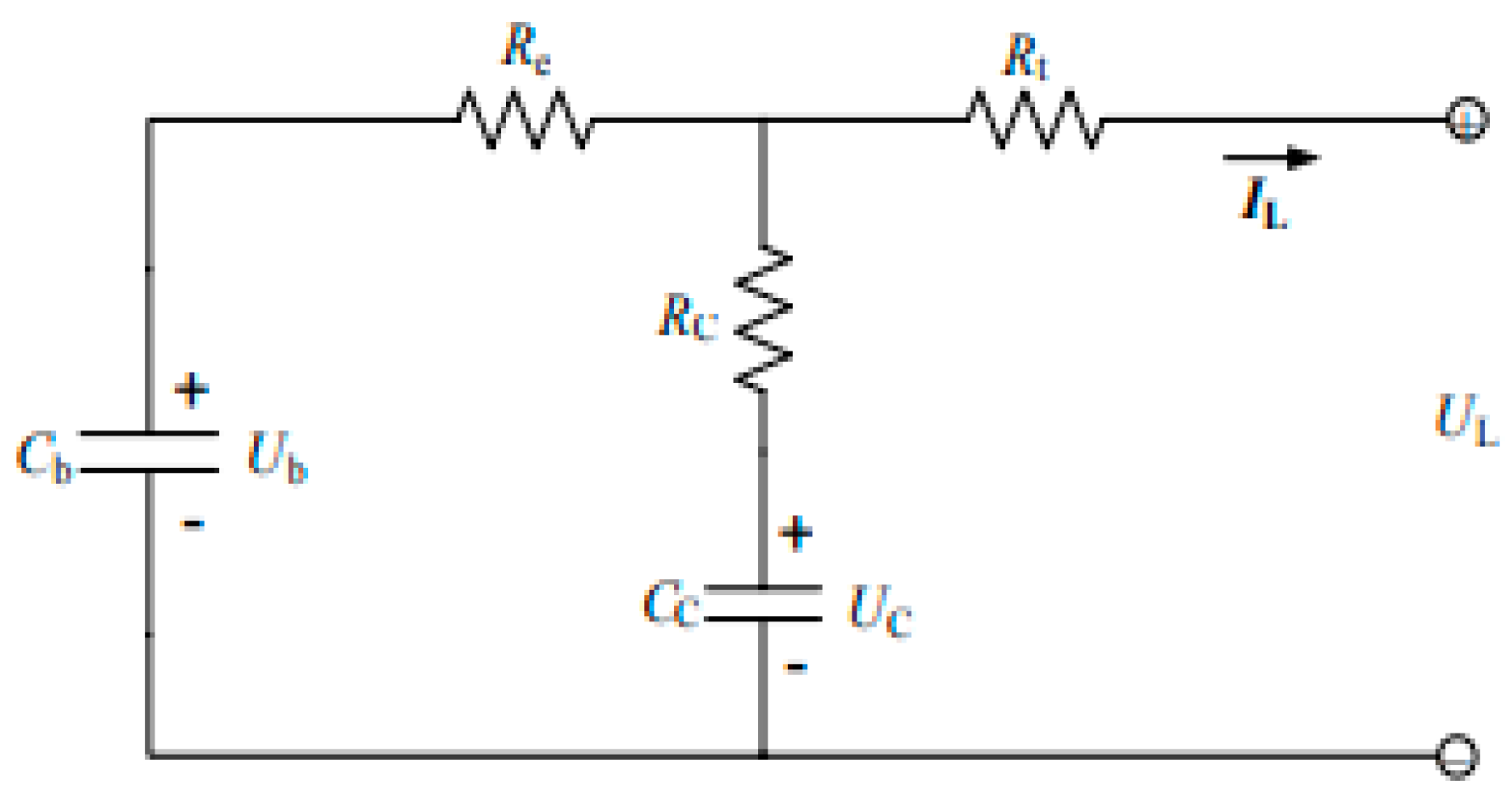
2.3.2. Equivalent Circuit Model
- Rint Model
- RC Model
- The Thevenin Model
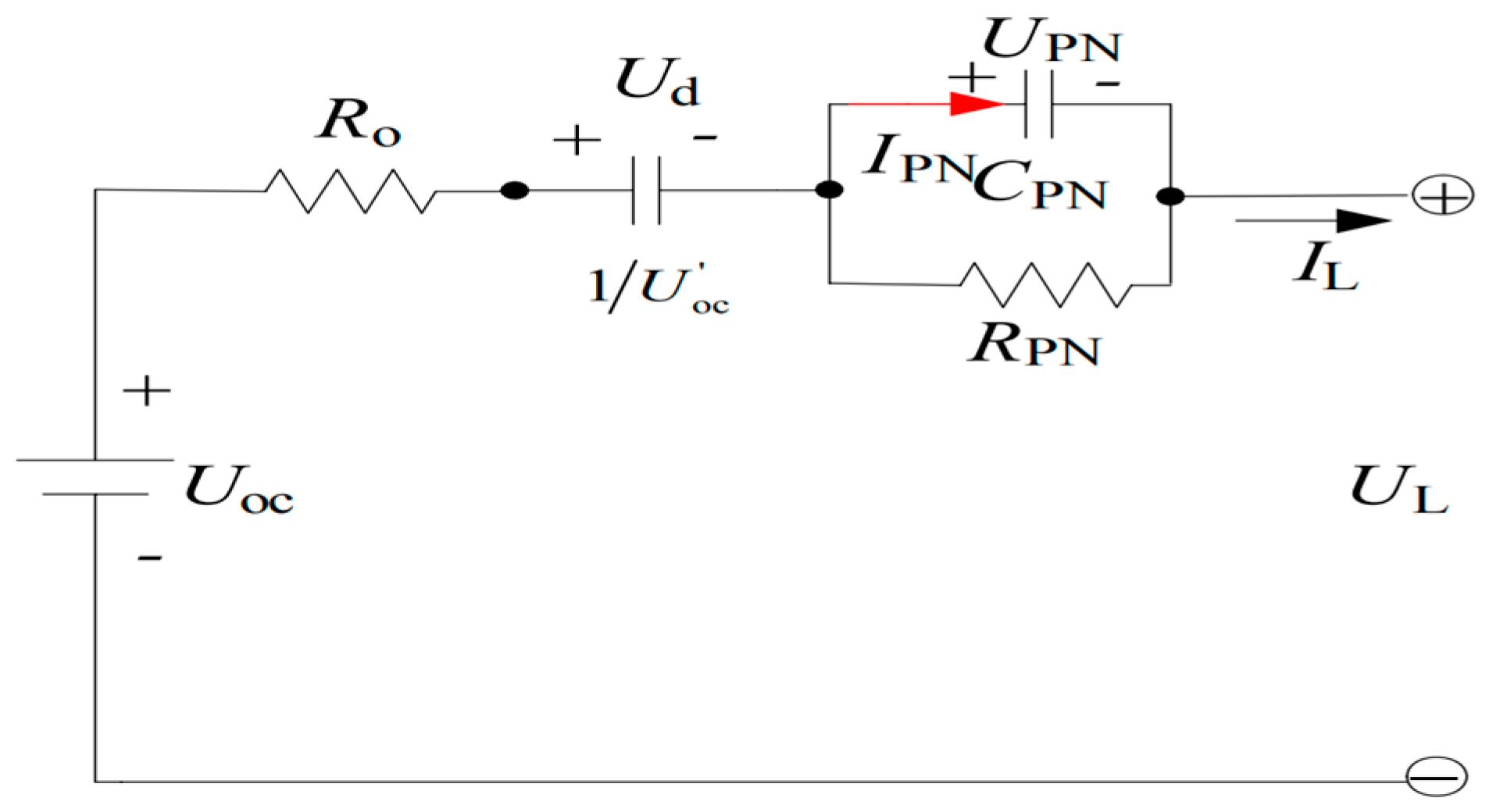
- The PNGV Model
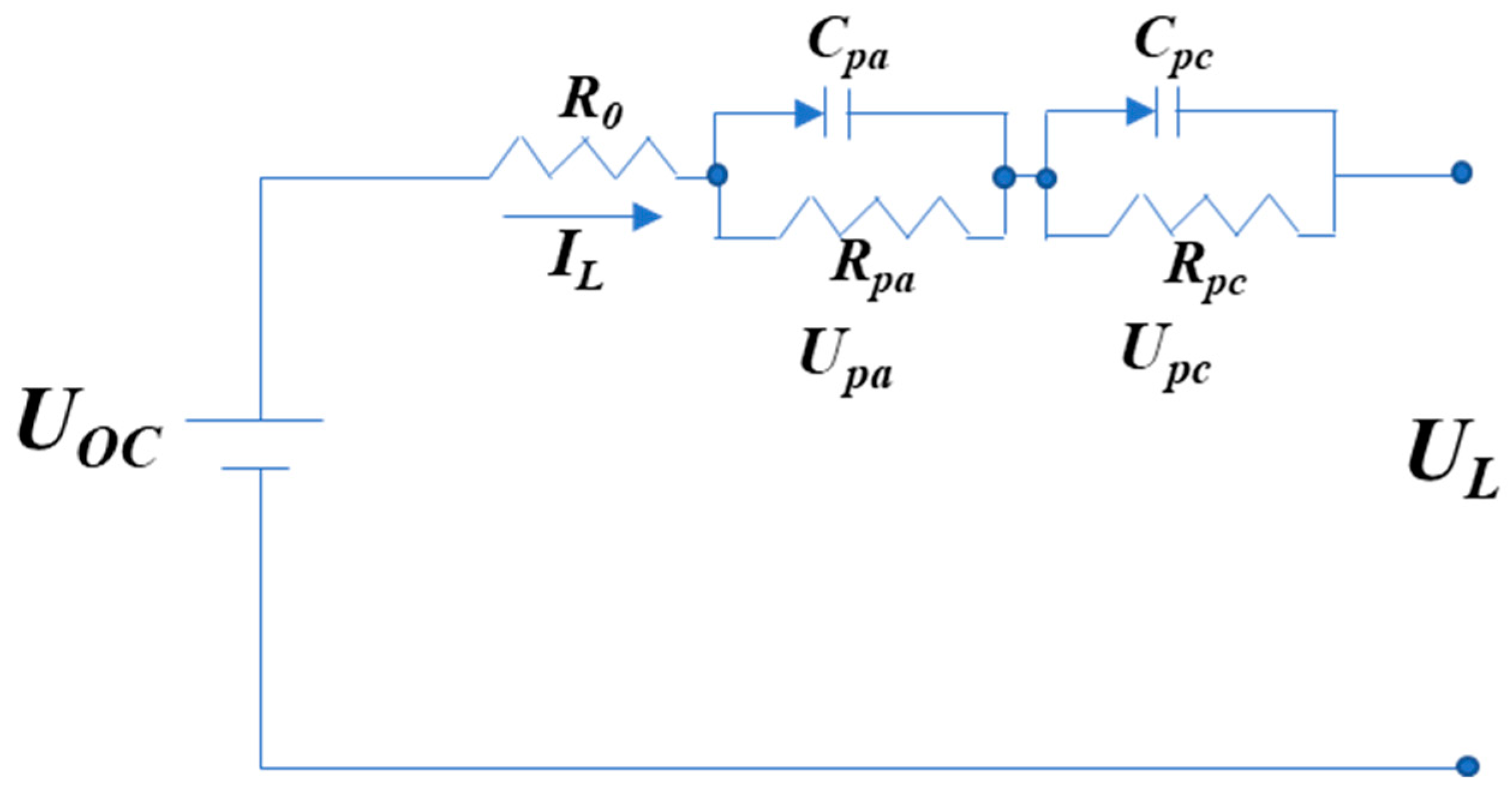
- The Dual Polarization (DP) Framework
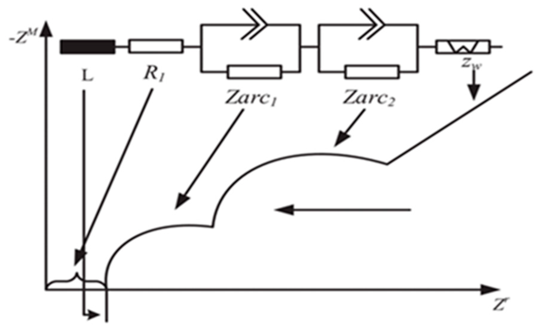
2.3.3. Electrochemical Impedance Model
2.4. Data-Driven Model Estimation
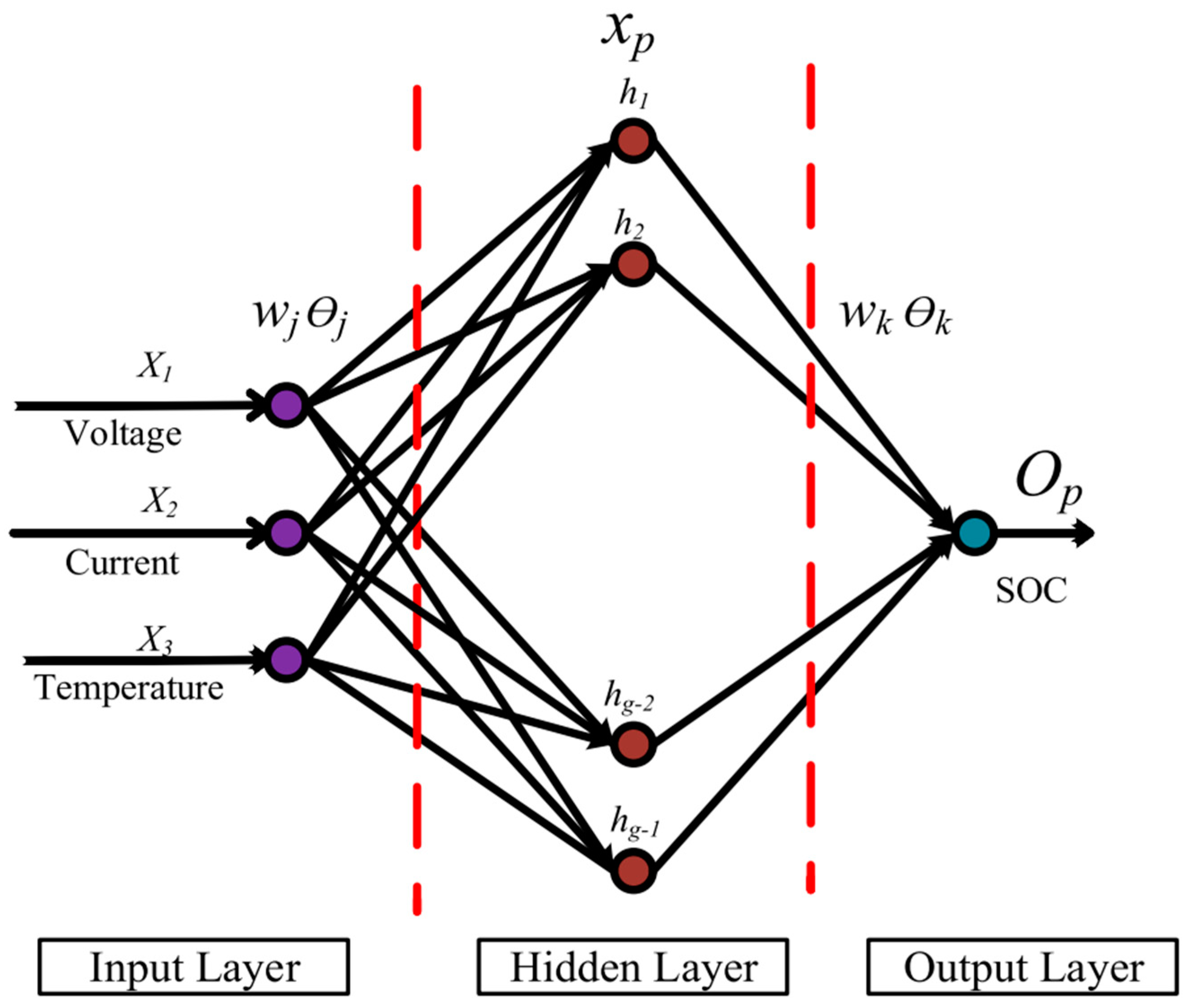
2.4.1. Neural Network Method
- Deep Neural Network
- Convolutional Neural Network
- Recurrent Neural Network
2.4.2. Deep Learning
2.4.3. Fuzzy Logic
3. SOH Estimation
3.1. Review of ML SOH Estimation Algorithm
3.1.1. Shallow Neural Network
3.1.2. Deep Learning Algorithm
3.1.3. Support Vector Machine
4. Challenges and Prospects
4.1. State of Charge Balancing Issues
4.2. Charging Strategy
4.3. Lithium-Ion Battery Material Issue
4.4. Hardware Development for Real-Time SOC Monitoring
4.5. Data Quality
4.6. Hyperparameter Tuning and Structure Selection
4.7. Hybrid Algorithms and Ensemble Learning
4.8. Evaluation and Implementation of the Algorithm
4.9. Thermal Influences
4.10. Sensor Constraints and Economic Factors
5. Conclusions
- Aging, discharge rates, and sensor precision all have an impact on the accumulated mistakes that plague coulomb counting.
- The OCV method’s flat SOC–OCV curve segment makes it inaccurate for LiFePO4 batteries and inapplicable in real time for EVs.
- The computing requirement and parameter estimation time provide difficulties for EM and ECM.
- Complex operations and sensitivity to model errors are KF’s limitations.
- NN requires extensive training, yet it produces reliable estimates in a variety of scenarios.
- The computational complexity and optimization difficulties of FL, ANFIS, GA, and PSO place limitations on them.
- Thorough research on electrochemical models to comprehend the dynamics and degradation of batteries.
- Creation of efficient SOC and SOH management controllers and real-time SOC and SOH estimation systems.
- Optimization-based reduction of computing complexity in data-driven approaches.
Author Contributions
Funding
Data Availability Statement
Acknowledgments
Conflicts of Interest
References
- Ramoni, M.O.; Zhang, H.-C. End-of-life (EOL) issues and options for electric vehicle batteries. Clean Technol. Environ. Policy 2013, 15, 881–891. [Google Scholar] [CrossRef]
- Hu, X.; Zou, C.; Zhang, C.; Li, Y. Technological developments in batteries: A survey of principal roles, types, and management needs. IEEE Power Energy Mag. 2017, 15, 20–31. [Google Scholar] [CrossRef]
- Xiong, R.; He, H.; Sun, F.; Zhao, K. Online estimation of peak power capability of Li-Ion batteries in electric vehicles by a hardware-in-loop approach. Energies 2012, 5, 1455–1469. [Google Scholar] [CrossRef]
- Xing, Y.; Ma, E.W.M.; Tsui, K.L.; Pecht, M. Battery management systems in electric and hybrid vehicles. Energies 2011, 4, 1840–1857. [Google Scholar] [CrossRef]
- Lillehei, C.; Cruz, A.B.; Johnsrude, I.; Sellers, R.D. A new method of assessing the state of charge of implanted cardiac pacemaker batteries. Am. J. Cardiol. 1965, 16, 717–721. [Google Scholar] [CrossRef]
- Hannan, M.A.; Lipu, M.S.H.; Hussain, A.; Mohamed, A. A review of lithium-ion battery state of charge estimation and management system in electric vehicle applications: Challenges and recommendations. Renew. Sustain. Energy Rev. 2017, 78, 834–854. [Google Scholar] [CrossRef]
- Li, Z.; Huang, J.; Liaw, B.Y.; Zhang, J. On state-of-charge determination for lithium-ion batteries. J. Power Sources 2017, 348, 281–301. [Google Scholar] [CrossRef]
- Kalawoun, J.; Biletska, K.; Suard, F.; Montaru, M. From a novel classification of the battery state of charge estimators toward a conception of an ideal one. J. Power Sources 2015, 279, 694–706. [Google Scholar] [CrossRef]
- Lu, L.; Han, X.; Li, J.; Hua, J.; Ouyang, M. A review on the key issues for lithium-ion battery management in electric vehicles. J. Power Sources 2013, 226, 272–288. [Google Scholar] [CrossRef]
- Plett, G.L. Battery Management and Control; ECE5720, Lecture Notes, Note 3; Artech House: Norwood, MA, USA, 2015; p. 7. [Google Scholar]
- Baccouche, I.; Jemmali, S.; Manai, B.; Omar, N.; Ben Amara, N.E. Improved OCV model of a Li-ion nmc battery for online SOC estimation using the extended Kalman filter. Energies 2017, 10, 764. [Google Scholar] [CrossRef]
- Lin, C.; Yu, Q.; Xiong, R.; Wang, L.Y. A study on the impact of open circuit voltage tests on state of charge estimation for lithium-ion batteries. Appl. Energy 2017, 205, 892–902. [Google Scholar] [CrossRef]
- Liu, K.; Li, K.; Peng, Q.; Zhang, C. A brief review on key technologies in the battery management system of electric vehicles. Front. Mech. Eng. 2018, 14, 47–64. [Google Scholar] [CrossRef]
- Zhang, B.; Lu, C.; Liu, J. Combination Algorithm for State of Charge Estimation. In Proceedings of the 2013 International Conference on Communication Systems and Network Technologies (CSNT 2013), Gwalior, India, 6–8 April 2013; pp. 865–867. [Google Scholar]
- Wenzel, M.J.; Drees, K.H.; Elbsat, M.N. Electrical Energy Storage System with Variable State-of-Charge Frequency Response Optimization. U.S. Patent 10186889B2, 22 January 2019. [Google Scholar]
- Grandjean, T.R.B.; McGordon, A.; Jennings, P.A. Structural identifiability of equivalent circuit models for Li-ion batteries. Energies 2017, 10, 90. [Google Scholar] [CrossRef]
- Tang, S.-X.; Camacho-Solorio, L.; Wang, Y.; Krstic, M. State-of-charge estimation from a thermal–electrochemical model of lithium-ion batteries. Automatica 2017, 83, 206–219. [Google Scholar] [CrossRef]
- Li, J.; Wang, L.; Lyu, C.; Pecht, M. State of charge estimation based on a simplified electrochemical model for a single LiCoO2 battery and battery pack. Energy 2017, 133, 572–583. [Google Scholar] [CrossRef]
- Wang, Y.; Zhang, C.; Chen, Z. On-line battery state-of-charge estimation based on an integrated estimator. Appl. Energy 2017, 185, 2026–2032. [Google Scholar] [CrossRef]
- Zou, C.; Manzie, C.; Nešić, D.; Kallapur, A.G. Multi-time-scale observer design for state-of-charge and state-of-health of a lithium-ion battery. J. Power Sources 2016, 335, 121–130. [Google Scholar] [CrossRef]
- Xiong, B.; Zhao, J.; Su, Y.; Wei, Z.; Skyllas-Kazacos, M. State of charge estimation of vanadium redox flow battery based on sliding mode observer and dynamic model including capacity fading factor. IEEE Trans. Sustain. Energy 2017, 8, 1658–1667. [Google Scholar] [CrossRef]
- Ye, M.; Guo, H.; Cao, B. A model-based adaptive state of charge estimator for a lithium-ion battery using an improved adaptive particle filter. Appl. Energy 2017, 190, 740–748. [Google Scholar] [CrossRef]
- Plett, G.L. Battery Management and Control; ECE5720, Lecture Notes, Note 2; Artech House: Norwood, MA, USA, 2015; p. 10. [Google Scholar]
- Kalman, R.E. A new approach to linear filtering and prediction problems. J. Basic Eng. 1960, 82, 35–45. [Google Scholar] [CrossRef]
- Plett, G.L. Kalman-Filter SOC Estimation for LiPB HEV Cells. In Proceedings of the 19th International Battery, Hybrid and Fuel Cell Electric Vehicle Symposium & Exhibition (EVS19), Busan, Republic of Korea, 19–23 October 2002; p. 3. [Google Scholar]
- Plett, G.L. Kalman-Filter SOC Estimation for LiPB HEV Cells. In Proceedings of the 19th International Battery, Hybrid and Fuel Cell Electric Vehicle Symposium & Exhibition (EVS19), Busan, Republic of Korea, 19–23 October 2002; p. 4. [Google Scholar]
- Haykin, S. (Ed.) Kalman Filtering and Neural Networks; Wiley Inter-Science: New York, NY, USA, 2001. [Google Scholar]
- Plett, G.L. Kalman-Filter SOC Estimation for LiPB HEV Cells. In Proceedings of the 19th International Battery, Hybrid and Fuel Cell Electric Vehicle Symposium & Exhibition (EVS19), Busan, Republic of Korea, 19–23 October 2002; p. 5. [Google Scholar]
- Rahman, A.; Anwar, S.; Izadian, A. Electrochemical model parameter identification of a lithium-ion battery using particle swarm optimization method. J. Power Sources 2016, 307, 86–97. [Google Scholar] [CrossRef]
- Sung, W.; Shin, C.B. Electrochemical model of a lithium-ion battery implemented into an automotive battery management system. Comput. Chem. Eng. 2015, 76, 87–97. [Google Scholar] [CrossRef]
- Peng, S.; Chen, C.; Shi, H.; Yao, Z. State of charge estimation of battery energy storage systems based on adaptive unscented Kalman filter with a noise statistics estimator. IEEE Access 2017, 5, 13202–13212. [Google Scholar] [CrossRef]
- Mastali, M.; Samadani, E.; Farhad, S.; Fraser, R.; Fowler, M. Three-dimensional multiparticle electrochemical model of LiFePO4 cells based on a resistor network methodology. Electrochim. Acta 2016, 190, 574–587. [Google Scholar] [CrossRef]
- Zou, C.; Manzie, C.; Nesic, D. A framework for simplification of PDE-based lithium-ion battery models. IEEE Trans. Control. Syst. Technol. 2015, 24, 1594–1609. [Google Scholar] [CrossRef]
- Bartlett, A.; Marcicki, J.; Onori, S.; Rizzoni, G.; Yang, X.G.; Miller, T. Electrochemical model-based state of charge and capacity estimation for a composite electrode lithium-Ion battery. IEEE Trans. Control Syst. Technol. 2015, 24, 384–399. [Google Scholar] [CrossRef]
- Zhang, L.; Wang, Z.; Hu, X.; Sun, F.; Dorrell, D.G. A comparative study of equivalent circuit models of ultracapacitors for electric vehicles. J. Power Sources 2015, 274, 899–906. [Google Scholar] [CrossRef]
- Zhang, X.; Lu, J.; Yuan, S.; Yang, J.; Zhou, X. A novel method for identification of lithium-ion battery equivalent circuit model parameters considering electrochemical properties. J. Power Sources 2017, 345, 21–29. [Google Scholar] [CrossRef]
- Widanage, W.D.; Barai, A.; Chouchelamane, G.H.; Uddin, K.; McGordon, A.; Marco, J.; Jennings, P. Design and use of multisite signals for Li-ion battery equivalent circuit modeling. Part 1: Signal design. J. Power Sources 2016, 324, 70–78. [Google Scholar] [CrossRef]
- Wang, Q.-K.; He, Y.-J.; Shen, J.-N.; Ma, Z.-F.; Zhong, G.-B. A unified modeling framework for lithium-ion batteries: An artificial neural network based thermal coupled equivalent circuit model approach. Energy 2017, 138, 118–132. [Google Scholar] [CrossRef]
- Deng, Z.; Yang, L.; Cai, Y.; Deng, H.; Sun, L. Online available capacity prediction and state of charge estimation based on advanced da-ta-driven algorithms for lithium iron phosphate battery. Energy 2016, 112, 469–480. [Google Scholar] [CrossRef]
- Plett, G.L. Battery Management and Control; ECE5720, Lecture Notes, Note 2; Artech House: Norwood, MA, USA, 2015; pp. 8–9. [Google Scholar]
- Lee, S.; Kim, J.; Lee, J.; Cho, B. State-of-charge and capacity estimation of lithium-ion battery using a new open-circuit voltage versus state-of-charge. J. Power Sources 2008, 185, 1367–1373. [Google Scholar] [CrossRef]
- Idaho National Engineering; Environmental Laboratory. Battery Test Manual for Plug-In Hybrid Electric Vehicles; Assistant Secretary for Energy Efficiency and Renewable Energy (EE); Idaho Operations Office: Idaho Falls, ID, USA, 2010. [Google Scholar]
- Lee, E.R.; Noh, H.; Park, B.U. Model selection via Bayesian information criterion for quantile regression models. J. Am. Stat. Assoc. 2014, 109, 216–229. [Google Scholar] [CrossRef]
- Hu, M.; Li, Y.; Li, S.; Fu, C.; Qin, D.; Li, Z. Lithium-ion battery modeling and parameter identification based on fractional theory. Energy 2018, 165, 153–163. [Google Scholar] [CrossRef]
- Zhang, J.; Wang, P.; Liu, Y.; Cheng, Z. Variable-Order Equivalent Circuit Modeling and State of Charge Estimation of Lithium-Ion Battery Based on Electrochemical Impedance Spectroscopy. Energies 2021, 14, 769. [Google Scholar] [CrossRef]
- Xu, J.; Mi, C.C.; Cao, B.; Cao, J. A new method to estimate the state of charge of lithium-ion batteries based on the battery impedance model. J. Power Sources 2013, 233, 277–284. [Google Scholar] [CrossRef]
- Li, M. Li-ion dynamics and state of charge estimation. Renew. Energy 2017, 100, 44–52. [Google Scholar] [CrossRef]
- Di Domenico, D.; Stefanopoulou, A.; Fiengo, G. Lithium-ion battery state of charge and critical surface charge estimation using an electrochemical model-based extended Kalman filter. J. Dyn. Syst. Meas. Control 2010, 132, 061302. [Google Scholar] [CrossRef]
- Cacciato, M.; Nobile, G.; Scarcella, G.; Scelba, G. Real-time model-based estimation of SoC and SOH for energy storage systems. IEEE Trans. Power Electron. 2017, 32, 794–803. [Google Scholar] [CrossRef]
- Ye, M.; Guo, H.; Xiong, R.; Yang, R. Model-based state-of-charge estimation approach of the lithium-ion battery using an improved adaptive particle filter. Energy Procedia 2016, 103, 394–399. [Google Scholar] [CrossRef]
- Xiong, R.; Cao, J.; Yu, Q.; He, H.; Sun, F. Critical review on the battery state of charge estimation methods for electric vehicles. IEEE Access 2017, 6, 1832–1843. [Google Scholar] [CrossRef]
- Dai, H.; Jiang, B.; Wei, X. Impedance characterization and modeling of lithium-ion batteries considering the internal temperature gradient. Energies 2018, 11, 220. [Google Scholar] [CrossRef]
- Chemali, E.; Kollmeyer, P.J.; Preindl, M.; Emadi, A. State-of-charge estimation of Li-ion batteries using deep neural networks: A machine learning approach. J. Power Sources 2018, 400, 242–255. [Google Scholar] [CrossRef]
- Lipu, M.S.H.; Hannan, M.A.; Hussain, A.; Saad, M.H.; Ayob, A.; Uddin, M.N. Extreme learning machine model for state-of-charge estimation of lithium-ion battery using gravitational search algorithm. IEEE Trans. Ind. Appl. 2019, 55, 4225–4234. [Google Scholar] [CrossRef]
- Hu, X.; Li, S.E.; Yang, Y. Advanced machine learning approach for lithium-ion battery state estimation in ELECTRIC VEHICLES. IEEE Trans. Transp. Electrif. 2015, 2, 140–149. [Google Scholar] [CrossRef]
- Giger, M.L. Machine learning in medical imaging. J. Amer. Coll. Radiol. 2018, 15, 512–520. [Google Scholar] [CrossRef]
- Chatzis, S.P.; Siakoulis, V.; Petropoulos, A.; Stavroulakis, E.; Vlachogiannakis, N. Forecasting stock market crisis events using deep and statistical machine learning techniques. Expert Syst. Appl. 2018, 112, 353–371. [Google Scholar] [CrossRef]
- Xu, Y.; Yang, C.; Zhong, J.; Wang, N.; Zhao, L. Robot teaching by teleoperation based on visual interaction and extreme learning machine. Neurocomputing 2017, 275, 2093–2103. [Google Scholar] [CrossRef]
- Silver, D.; Huang, A.; Maddison, C.J.; Guez, A.; Sifre, L.; van den Driessche, G.; Schrittwieser, J.; Antonoglou, I.; Panneershelvam, V.; Lanctot, M.; et al. Mastering the game of Go with deep neural networks and tree search. Nature 2016, 529, 484–489. [Google Scholar] [CrossRef]
- Anand, I.; Mathur, B. State of charge estimation of lead acid batteries using neural networks. In Proceedings of the 2013 International Conference on Circuits, Power and Computing Technologies (ICCPCT), Nagercoil, India, 20–21 March 2013; pp. 596–599. [Google Scholar]
- Chen, J.; Longhui, W.; Wu, C.; Yiheng, Z. Method for Estimating State of Charge of Battery. WO Patent 2019052015A1, 21 March 2019. [Google Scholar]
- Hannan, M.A.; Lipu, M.S.H.; Hussain, A.; Saad, M.H.; Ayob, A. Neural network approach for estimating state of charge of lithium-ion battery using backtracking search algorithm. IEEE Access 2018, 6, 10069–10079. [Google Scholar] [CrossRef]
- Hongwei, L.; Caiying, S. Methods of State of Charge Estimation of Electric Vehicle. Automot. Eng. 2017, 31–33. [Google Scholar]
- Xia, B.; Cui, D.; Sun, Z.; Lao, Z.; Zhang, R.; Wang, W.; Sun, W.; Lai, Y.; Wang, M. State of charge estimation of lithium-ion batteries using optimized Levenberg-Marquardt wavelet neural network. Energy 2018, 153, 694–705. [Google Scholar] [CrossRef]
- Schmidhuber, J. Deep learning in neural networks: An overview. Neural Netw. 2015, 61, 85–117. [Google Scholar] [CrossRef] [PubMed]
- He, W.; Williard, N.; Chen, C.; Pecht, M. State of charge estimation for Li-ion batteries using neural network modeling and unscented Kalman filter-based error cancellation. Int. J. Electr. Power Energy Syst. 2014, 62, 783–791. [Google Scholar] [CrossRef]
- Crocioni, G.; Pau, D.; Delorme, J.-M.; Gruosso, G. Li-ion batteries parameter estimation with tiny neural networks embedded on intelligent IoT microcontrollers. IEEE Access 2020, 8, 122135–122146. [Google Scholar] [CrossRef]
- Song, X.; Yang, F.; Wang, D.; Tsui, K.-L. Combined CNN-LSTM network for state-of-charge estimation of lithium-ion batteries. IEEE Access 2019, 7, 88894–88902. [Google Scholar] [CrossRef]
- Huang, Z.; Yang, F.; Xu, F.; Song, X.; Tsui, K.-L. Convolutional gated recurrent unit–recurrent neural network for state-of-charge estimation of lithium-ion batteries. IEEE Access 2019, 7, 93139–93149. [Google Scholar] [CrossRef]
- Hannan, M.A.; How, D.N.T.; Lipu, M.S.H.; Ker, P.J.; Dong, Z.Y.; Mansur, M.; Blaabjerg, F. SOC estimation of Li-ion batteries with learning rate-optimized deep fully convolutional network. IEEE Trans. Power Electron. 2020, 36, 7349–7353. [Google Scholar] [CrossRef]
- Hu, J.; Hu, J.; Lin, H.; Li, X.; Jiang, C.; Qiu, X.; Li, W. State-of-charge estimation for battery management system using optimized support vector machine for regression. J. Power Sources 2014, 269, 682–693. [Google Scholar] [CrossRef]
- Jiménez-Bermejo, D.; Fraile-Ardanuy, J.; Castaño-Solis, S.; Merino, J.; Álvaro-Hermana, R. Using dynamic neural networks for battery state of charge estimation in electric vehicles. Procedia Comput. Sci. 2018, 130, 533–540. [Google Scholar] [CrossRef]
- Lipu, M.S.H.; Hussain, A.; Saad, M.H.M.; Ayob, A.; Hannan, M.A. Improved recurrent NARX neural network model for state of charge estimation of lithium-ion battery using pso algorithm. In Proceedings of the 2018 IEEE Symposium on Computer Applications & Industrial Electronics (ISCAIE), Penang, Malaysia, 28–29 April 2018; pp. 354–359. [Google Scholar]
- Sun, W.; Qiu, Y.; Sun, L.; Hua, Q. Neural network-based learning and estimation of batterystate-of-charge: A comparison study between direct and indirect methodology. Int. J. Energy Res. 2020, 44, 10307–10319. [Google Scholar] [CrossRef]
- Qin, X.; Gao, M.; He, Z.; Liu, Y. State of charge estimation for lithium-ion batteries based on NARX neural network and UKF. In Proceedings of the 2019 IEEE 17th International Conference on Industrial Informatics (INDIN), Helsinki-Espoo, Finland, 22–25 July 2019; pp. 1706–1711. [Google Scholar]
- Wang, Q.; Gu, H.; Ye, M.; Wei, M.; Xu, X. State of charge estimation for lithium-ion battery based on NARX recurrent neural network and moving window method. IEEE Access 2021, 9, 83364–83375. [Google Scholar] [CrossRef]
- Vapnik, V. The Support Vector Method of Function Estimation. In Nonlinear Modeling; Springer: Boston, MA, USA, 1998; pp. 55–85. [Google Scholar] [CrossRef]
- Fletcher, T. Support vector machines explained. Tutor. Pap. 2009, 1118, 1–19. Available online: http://sutikno.blog.undip.ac.id/files/2011/11/SVM-Explained.pdf (accessed on 12 January 2025).
- Antón, J.C.; Nieto, P.J.G.; Viejo, C.B.; Vilán, J.A.V. Support vector machines used to estimate the battery state of charge. IEEE Trans. Power Electron. 2013, 28, 5919–5926. [Google Scholar] [CrossRef]
- Li, R.; Xu, S.; Li, S.; Zhou, Y.; Zhou, K.; Liu, X.; Yao, J. State of charge prediction algorithm of lithium-ion battery based on PSO-SVR cross validation. IEEE Access 2020, 8, 10234–10242. [Google Scholar] [CrossRef]
- Novák, V.; Perfilieva, I.; Močkoř, J. Functional systems in fuzzy logic theories. In Mathematical Principles of Fuzzy Logic; Springer: Boston, MA, USA, 1999; pp. 179–222. [Google Scholar]
- Salkind, A.J.; Fennie, C.; Singh, P.; Atwater, T.; E Reisner, D. Determination of state-of-charge and state-of-health of batteries by fuzzy logic methodology. J. Power Sources 1999, 80, 293–300. [Google Scholar] [CrossRef]
- Sheng, H.; Xiao, J. Electric vehicle state of charge estimation: Nonlinear correlation and fuzzy support vector machine. J. Power Sources 2015, 281, 131–137. [Google Scholar] [CrossRef]
- Li, Y.; Wang, C.; Gong, J. A combination Kalman filter approach for state of charge estimation of lithium-ion battery considering model uncertainty. Energy 2016, 109, 933–946. [Google Scholar] [CrossRef]
- Singh, P.; Vinjamuri, R.; Wang, X.; Reisner, D. Design and implementation of a fuzzy logic-based state-of-charge meter for Li-ion batteries used in portable defibrillators. J. Power Sources 2006, 162, 829–836. [Google Scholar] [CrossRef]
- Awadallah, M.A.; Venkatesh, B. Accuracy improvement of SoC estimation in lithium-ion batteries. J. Energy Storage 2016, 6, 95–104. [Google Scholar] [CrossRef]
- Zahid, T.; Xu, K.; Li, W.; Li, C.; Li, H. State of charge estimation for electric vehicle power battery using advanced machine learning algorithm under diversified drive cycles. Energy 2018, 162, 871–882. [Google Scholar] [CrossRef]
- Shen, W.; Chan, C.; Lo, E.; Chau, K. Adaptive neurofuzzy modeling of battery residual capacity for electric vehicles. IEEE Trans. Ind. Electron. 2002, 49, 677–684. [Google Scholar] [CrossRef]
- Arabmakki, E.; Kantardzic, M. SOM-based partial labeling of imbalanced data stream. Neurocomputing 2017, 262, 120–133. [Google Scholar] [CrossRef]
- Coleman, M.; Hurley, W.G.; Lee, C.K. An improved battery characterization method using a two-pulse load test. IEEE Trans. Energy Convers. 2008, 23, 708–713. [Google Scholar] [CrossRef]
- Roscher, M.A.; Assfalg, J.; Bohlen, O.S. Detection of utilizable capacity deterioration in battery systems. IEEE Trans. Veh. Technol. 2010, 60, 98–103. [Google Scholar] [CrossRef]
- Zhang, J.; Lee, J. A review on prognostics and health monitoring of Li-ion battery. J. Power Sources 2011, 196, 6007–6014. [Google Scholar] [CrossRef]
- Xiong, R.; Tian, J.; Mu, H.; Wang, C. A systematic model-based degradation behavior recognition and health monitoring method for lithium-ion batteries. Appl. Energy 2017, 207, 372–383. [Google Scholar] [CrossRef]
- Berecibar, M.; Gandiaga, I.; Villarreal, I.; Omar, N.; Van Mierlo, J.; van den Bossche, P. Critical review of state of health estimation methods of Li-ion batteries for real applications. Renew. Sustain. Energy Rev. 2016, 56, 572–587. [Google Scholar] [CrossRef]
- Nejad, S.; Gladwin, D.; Stone, D. A systematic review of lumped-parameter equivalent circuit models for real-time estimation of lithium-ion battery states. J. Power Sources 2016, 316, 183–196. [Google Scholar] [CrossRef]
- Wang, D.; Yang, F.; Tsui, K.-L.; Zhou, Q.; Bae, S.J. Remaining useful life prediction of lithium-ion batteries based on spherical cubature particle filter. IEEE Trans. Instrum. Meas. 2016, 65, 1282–1291. [Google Scholar] [CrossRef]
- Plett, G.L. Sigma-point Kalman filtering for battery management systems of LiPB-based HEV battery packs: Part 1: Intro-duction and state estimation. J. Power Sources 2006, 161, 1356–1368. [Google Scholar] [CrossRef]
- Hu, C.; Youn, B.D.; Chung, J.S.; Ortanez, R. A multiscale framework with extended kalman filter for lithium-ion battery SOC and capacity estimation. ECS Meet. Abstr. 2010, 92, 694–704. [Google Scholar] [CrossRef]
- Wang, J.; Liu, P.; Hicks-Garner, J.; Sherman, E.; Soukiazian, S.; Verbrugge, M.; Tataria, H.; Musser, J.; Finamore, P. Cycle-life model for graphiteLiFePO4 cells. J. Power Sources 2010, 196, 3942–3948. [Google Scholar] [CrossRef]
- Todeschini, F.; Onori, S.; Rizzoni, G. An experimentally validated capacity degradation model for Li-ion batteries in PHEVs applications. IFAC Proc. Vol. 2012, 45, 456–461. [Google Scholar] [CrossRef]
- Omar, N.; Monem, M.A.; Firouz, Y.; Salminen, J.; Smekens, J.; Hegazy, O.; Gaulous, H.; Mulder, G.; Van Den Bossche, P.; Coosemans, T.; et al. Lithium iron phosphate based battery—Assessment of the aging parameters and development of cycle life model. Appl. Energy 2014, 113, 1575–1585. [Google Scholar] [CrossRef]
- Ecker, M.; Gerschler, J.B.; Vogel, J.; Käbitz, S.; Hust, F.; Dechent, P.; Sauer, D.U. Development of a lifetime prediction model for lithium-ion batteries based on extended accelerated aging test data. J. Power Sources 2012, 215, 248–257. [Google Scholar] [CrossRef]
- Ouyang, M.; Feng, X.; Han, X.; Lu, L.; Li, Z.; He, X. A dynamic capacity degradation model and its applications considering varying load for a large format Li-ion battery. Appl. Energy 2016, 165, 48–59. [Google Scholar] [CrossRef]
- Gao, Y.; Jiang, J.; Zhang, C.; Zhang, W.; Ma, Z.; Jiang, Y. Lithium-ion battery aging mechanisms and life model under different charging stresses. J. Power Sources 2017, 356, 103–114. [Google Scholar] [CrossRef]
- Rezvanizaniani, S.M.; Liu, Z.; Chen, Y.; Lee, J. Review and recent advances in battery health monitoring and prognostics technologies for electric vehicle (EV) safety and mobility. J. Power Sources 2014, 256, 110–124. [Google Scholar] [CrossRef]
- Hu, C.; Jain, G.; Zhang, P.; Schmidt, C.; Gomadam, P.; Gorka, T. Data-driven method based on particle swarm optimization and k-nearest neighbor regression for estimating capacity of lithium-ion battery. Appl. Energy 2014, 129, 49–55. [Google Scholar] [CrossRef]
- Liu, D.; Zhou, J.; Liao, H.; Peng, Y.; Peng, X. A health indicator extraction and optimization framework for lithium-ion battery degradation modeling and prognostics. IEEE Trans. Syst. Man Cybern. Syst. 2015, 45, 915–928. [Google Scholar] [CrossRef]
- Klass, V.; Behm, M.; Lindbergh, G. A support vector machine-based state-of-health estimation method for lithium-ion batteries under electric vehicle operation. J. Power Sources 2014, 270, 262–272. [Google Scholar] [CrossRef]
- You, G.-W.; Park, S.; Oh, D. Real-time state-of-health estimation for electric vehicle batteries: A data-driven approach. Appl. Energy 2016, 176, 92–103. [Google Scholar] [CrossRef]
- Kashkooli, A.G.; Fathiannasab, H.; Mao, Z.; Chen, Z. Application of artificial intelligence to state-of-charge and state-of-health estimation of calendar-aged lithium-ion pouch cells. J. Electrochem. Soc. 2019, 166, A605–A615. [Google Scholar] [CrossRef]
- Mao, L.; Hu, H.; Chen, J.; Zhao, J.; Qu, K.; Jiang, L. Online state-of-health estimation method for lithium-ion battery based on CEEMDAN for feature analysis and RBF neural network. IEEE J. Emerg. Sel. Top. Power Electron. 2021, 11, 187–200. [Google Scholar] [CrossRef]
- Lin, M.; Zeng, X.; Wu, J. State of health estimation of lithium-ion battery based on an adaptive tunable hybrid radial basis function network. J. Power Sources 2021, 504, 230063. [Google Scholar] [CrossRef]
- Saha, B.; Goebel, K.; Poll, S.; Christophersen, J. Prognostics methods for battery health monitoring using a bayesian framework. IEEE Trans. Instrum. Meas. 2008, 58, 291–296. [Google Scholar] [CrossRef]
- Zhang, S.; Zhai, B.; Guo, X.; Wang, K.; Peng, N.; Zhang, X. Synchronous estimation of state of health and remaining useful lifetime for lithium-ion battery using the incremental capacity and artificial neural networks. J. Energy Storage 2019, 26, 100951. [Google Scholar] [CrossRef]
- Xia, Z.; Abu Qahouq, J.A. Lithium-ion battery ageing behavior pattern characterization and state-of-health estimation using data-driven method. IEEE Access 2021, 9, 98287–98304. [Google Scholar] [CrossRef]
- Shi, Y.; Ahmad, S.; Tong, Q.; Lim, T.M.; Wei, Z.; Ji, D.; Eze, C.M.; Zhao, J. The optimization of state of charge and state of health estimation for lithium-ions battery using combined deep learning and Kalman filter methods. Int. J. Energy Res. 2021, 45, 11206–11230. [Google Scholar] [CrossRef]
- Liu, Z.; Zhao, J.; Wang, H.; Yang, C. A new lithium-ion battery SOH estimation method based on an indirect enhanced health indicator and support vector regression in PHMs. Energies 2020, 13, 830. [Google Scholar] [CrossRef]
- Feng, X.; Weng, C.; He, X.; Wang, L.; Ren, D.; Lu, L.; Han, X.; Ouyang, M. Incremental capacity analysis on commercial lithium-ion batteries using support vector regression: A parametric study. Energies 2018, 11, 2323. [Google Scholar] [CrossRef]
- Guo, Y.; Huang, K.; Hu, X. A state-of-health estimation method of lithium-ion batteries based on multi-feature extracted from constant current charging curve. J. Energy Storage 2021, 36, 102372. [Google Scholar] [CrossRef]
- Widodo, A.; Shim, M.-C.; Caesarendra, W.; Yang, B.-S. Intelligent prognostics for battery health monitoring based on sample entropy. Expert Syst. Appl. 2011, 38, 11763–11769. [Google Scholar] [CrossRef]
- Cai, L.; Meng, J.; Stroe, D.-I.; Luo, G.; Teodorescu, R. An evolutionary framework for lithium-ion battery state of health estimation. J. Power Sources 2018, 412, 615–622. [Google Scholar] [CrossRef]
- Yang, D.; Wang, Y.; Pan, R.; Chen, R.; Chen, Z. State-of-health estimation for the lithium-ion battery based on support vector regression. Appl. Energy 2018, 227, 273–283. [Google Scholar] [CrossRef]
- Ma, C.; Zhai, X.; Wang, Z.; Tian, M.; Yu, Q.; Liu, L.; Liu, H.; Wang, H.; Yang, X. State of health prediction for lithium-ion batteries using multiple-view feature fusion and support vector regression ensemble. Int. J. Mach. Learn. Cybern. 2018, 10, 2269–2282. [Google Scholar] [CrossRef]
- Xiong, W.; Mo, Y.; Yan, C. Online state-of-health estimation for second-use lithium-ion batteries based on weighted least squares support vector machine. IEEE Access 2020, 9, 1870–1881. [Google Scholar] [CrossRef]
- Dai, H.; Wei, X.; Sun, Z.; Wang, J.; Gu, W. Online cell SOC estimation of Li-ion battery packs using a dual time-scale Kalman filtering for EV applications. Appl. Energy 2012, 95, 227–237. [Google Scholar] [CrossRef]
- Lin, Q.; Wang, J.; Xiong, R.; Shen, W.; He, H. Towards a smarter battery management system: A critical review on optimal charging methods of lithium ion batteries. Energy 2019, 183, 220–234. [Google Scholar] [CrossRef]
- Collin, R.; Miao, Y.; Yokochi, A.; Enjeti, P.; von Jouanne, A. Advanced electric vehicle fast-charging technologies. Energies 2019, 12, 1839. [Google Scholar] [CrossRef]
- Zhang, R.; Xia, B.; Li, B.; Cao, L.; Lai, Y.; Zheng, W.; Wang, H.; Wang, W. State of the art of lithium-ion battery SOC estimation for electrical vehicles. Energies 2018, 11, 1820. [Google Scholar] [CrossRef]
- Chaoui, H.; Ibe-Ekeocha, C.C. State of charge and state of health estimation for lithium batteries using recurrent neural networks. IEEE Trans. Veh. Technol. 2017, 66, 8773–8783. [Google Scholar] [CrossRef]
- Zhang, Y.; Xiong, R.; He, H.; Shen, W. Lithium-ion battery pack state of charge and state of energy estimation algorithms using a hardwarein-the-loop validation. IEEE Trans. Power Electron. 2017, 32, 4421–4431. [Google Scholar] [CrossRef]
- Chen, C.; Xiong, R.; Shen, W. A lithium-ion battery-in-the-loop approach to test and validate multiscale dual H infinity filters for state-of charge and capacity estimation. IEEE Trans. Power Electron. 2018, 33, 332–342. [Google Scholar] [CrossRef]
- Tian, X.; Jeppesen, B.; Ikushima, T.; Baronti, F.; Morello, R. Accelerating State-Of-Charge Estimation in FPGA-based Battery Management Systems. In Proceedings of the 6th Hybrid and Electric Vehicles Conference (HEVC 2016), London, UK, 2–3 November 2016; pp. 4–6. [Google Scholar]
- Sahinoglu, G.O.; Pajovic, M.; Sahinoglu, Z.; Wang, Y.; Orlik, P.V.; Wada, T. Battery state-of-charge estimation based on regular/recurrent gaussian process regression. IEEE Trans. Ind. Electron. 2017, 65, 4311–4321. [Google Scholar] [CrossRef]
- Zhao, L.; Yao, W.; Wang, Y.; Hu, J. Machine learning-based method for remaining range prediction of electric vehicles. IEEE Access 2020, 8, 212423–212441. [Google Scholar] [CrossRef]
- Zhu, S.; Han, J.; An, H.-Y.; Pan, T.-S.; Wei, Y.-M.; Song, W.-L.; Chen, H.-S.; Fang, D. A novel embedded method for in-situ measuring internal multi-point temperatures of lithium ion batteries. J. Power Sources 2020, 456, 227981. [Google Scholar] [CrossRef]
- Peng, J.; Zhou, X.; Jia, S.; Jin, Y.; Xu, S.; Chen, J. High precision strain monitoring for lithium ion batteries based on fiber Bragg grating sensors. J. Power Sources 2019, 433, 226692. [Google Scholar] [CrossRef]
- Teoh, E.J.; Tan, K.C.; Xiang, C. Estimating the number of hidden neurons in a feedforward network using the singular value decomposition. IEEE Trans. Neural Netw. 2006, 17, 1623–1629. [Google Scholar] [CrossRef]
- Cui, Z.; Wang, L.; Li, Q.; Wang, K. A comprehensive review on the state of charge estimation for lithium-ion battery based on neural network. Int. J. Energy Res. 2021, 46, 5423–5440. [Google Scholar] [CrossRef]
- Shen, S.; Sadoughi, M.; Li, M.; Wang, Z.; Hu, C. Deep convolutional neural networks with ensemble learning and transfer learning for capacity estimation of lithium-ion batteries. Appl. Energy 2020, 260, 114296. [Google Scholar] [CrossRef]
- Li, Y.; Zou, C.; Berecibar, M.; Nanini-Maury, E.; Chan, J.C.-W.; Bossche, P.v.D.; Van Mierlo, J.; Omar, N. Random forest regression for online capacity estimation of lithium-ion batteries. Appl. Energy 2018, 232, 197–210. [Google Scholar] [CrossRef]
- Xu, H.; Peng, Y.; Su, L. Health state estimation method of lithium ion battery based on NASA experimental data set. IOP Conf. Ser. Mater. Sci. Eng. 2018, 452, 032067. [Google Scholar] [CrossRef]
- Kollmeyer, P. Panasonic 18650PF li-ion battery data. In Mendeley Data; Elsevier Inc: Amsterdam, The Netherlands, 2018; Volume 1. [Google Scholar] [CrossRef]
- Naguib, M.; Kollmeyer, P.; Skells, M. LG 18650hg2 li-ion battery data and example deep neural network xEV SOC estimator script. Mendeley Data 2020, 3, 2020. [Google Scholar] [CrossRef]
- Saha, K.; Goebel, B. Battery Data Set. NASA Ames Prognostics Data Repository; NASA Ames: Moffett Field, CA, USA, 2007. Available online: http://ti.arc.nasa.gov/project/prognostic-data-repository (accessed on 12 January 2025).
- Feng, X.; Chen, J.; Zhang, Z.; Miao, S.; Zhu, Q. State-of-charge estimation of lithium-ion battery based on clockwork recurrent neural network. Energy 2021, 236, 121360. [Google Scholar] [CrossRef]
- Yang, F.; Song, X.; Xu, F.; Tsui, K.-L. State-of-charge estimation of lithium-ion batteries via long short-term memory network. IEEE Access 2019, 7, 53792–53799. [Google Scholar] [CrossRef]
- Bhattacharjee, A.; Verma, A.; Mishra, S.; Saha, T.K. Estimating state of charge for xEV batteries using 1D convolutional neural networks and transfer learning. IEEE Trans. Veh. Technol. 2021, 70, 3123–3135. [Google Scholar] [CrossRef]
- Kim, S.; Choi, Y.Y.; Kim, K.J.; Choi, J.-I. Forecasting state-of-health of lithium-ion batteries using variational long short-term memory with transfer learning. J. Energy Storage 2021, 41, 102893. [Google Scholar] [CrossRef]


| Algorithm | Input | Output | Metric | Hyperparameter | Data Profile |
|---|---|---|---|---|---|
| Linear Regression (LR) | Voltage, Current, Temperature | SOC | RMSE Root Mean Squared Error, MSE Mean Squared Error MAE Mean Absolute Error | Learning Rate (LR), Regularization (REG) | Cycles, Temperature Variant |
| Support Vector Machine (SVM) | Voltage, Current, Temperature | SOC | Accuracy, Precision, Recall | Kernel, C, Gamma (γ) | Cycles, Load prof |
| Back-Propagation Neural Network (BPNN) | Voltage, Current, Temperature | SOC | Coefficient of Determination R², MSE, RMSE | LR, Momentum (MOM), Layers | Lab, Driving past |
| Recurrent Neural Network (RNN) | Voltage, Current, Temperature | SOC | Accuracy, RMSE, MAE | RNN Layers, Cells | Seq data, Temp Corr |
| Adaptive Neuro-Fuzzy Inference System (ANSFIS) | Voltage, Current, Temperature | SOC | Rule Accuracy, RMSE | Rules, Membership Functions (MFs) | Expert knows, Fuzzy rules |
| Nonlinear Autoregressive with Exogenous Input Neural Network (NARXNN) | Voltage, Current, Temperature | SOC | R², MSE, Accuracy | Delays, Neurons | Series, Feedback loops |
| Genetic Algorithm (GA) | Voltage, Current, Temperature | SOC | Conversion Rate, Accuracy | Population Size (POP Size), Mutation Rate (Mut), Crossover Rate (Xover) | Param opt, Feature sel |
| Fuzzy Logic (FL) | Voltage, Current, Temperature | SOC | Rule Accuracy, Interpretability | MFs, Rule Base | Expert knows, Op data |
| Long Short-Term Memory (LSTM) | Voltage, Current, Temperature | SOC | Accuracy, RMSE, MAE | LR, Units, Dropout | Series, Charge/discharge |
| Gradient Boosting Machines (GBM) | Voltage, Current, Temperature | SOC | MAE, RMSE, R² | LR, Estimators, Depth | Cycles, Aging data |
| Random Forest (RF) | Voltage, Current, Temperature | SOC | R², MSE, RMSE | Trees, Depth, Split | Lab, Real-world use |
| Reinforcement Learning | Voltage, Current, Temperature | SOC | Reward, Error Rate | Learning Rate, Discount Factor | Simulated environments |
| PCA + ML Model | Voltage, Current, Temperature | SOC | R², MSE, RMSE | Components, ML Hyperparameters | Noise-reduced data |
| Ensemble Methods | Voltage, Current, Temperature | SOC | Accuracy, RMSE, R² | Number of Models, Strategy | Diverse driving patterns |
| Deep Belief Networks | Voltage, Current, Temperature | SOC | R², MSE, MAE | Layers, LR, Epochs | Multivariate time series |
| Convolutional NN | Voltage, Current, Temperature | SOC | Accuracy, Precision, Recall | Filters, Kernel Size | Image, Sequential data |
| k-NN | Voltage, Current, Temperature | SOC | Accuracy, RMSE, Precision | Number of Neighbors | Cycles, Driving conditions |
| Decision Trees | Voltage, Current, Temperature | SOC | Accuracy, R², RMSE | Depth, Min Samples | Cycles, Varied temps |
Disclaimer/Publisher’s Note: The statements, opinions and data contained in all publications are solely those of the individual author(s) and contributor(s) and not of MDPI and/or the editor(s). MDPI and/or the editor(s) disclaim responsibility for any injury to people or property resulting from any ideas, methods, instructions or products referred to in the content. |
© 2025 by the authors. Licensee MDPI, Basel, Switzerland. This article is an open access article distributed under the terms and conditions of the Creative Commons Attribution (CC BY) license (https://creativecommons.org/licenses/by/4.0/).
Share and Cite
Soyoye, B.D.; Bhattacharya, I.; Anthony Dhason, M.V.; Banik, T. State of Charge and State of Health Estimation in Electric Vehicles: Challenges, Approaches and Future Directions. Batteries 2025, 11, 32. https://doi.org/10.3390/batteries11010032
Soyoye BD, Bhattacharya I, Anthony Dhason MV, Banik T. State of Charge and State of Health Estimation in Electric Vehicles: Challenges, Approaches and Future Directions. Batteries. 2025; 11(1):32. https://doi.org/10.3390/batteries11010032
Chicago/Turabian StyleSoyoye, Babatunde D., Indranil Bhattacharya, Mary Vinolisha Anthony Dhason, and Trapa Banik. 2025. "State of Charge and State of Health Estimation in Electric Vehicles: Challenges, Approaches and Future Directions" Batteries 11, no. 1: 32. https://doi.org/10.3390/batteries11010032
APA StyleSoyoye, B. D., Bhattacharya, I., Anthony Dhason, M. V., & Banik, T. (2025). State of Charge and State of Health Estimation in Electric Vehicles: Challenges, Approaches and Future Directions. Batteries, 11(1), 32. https://doi.org/10.3390/batteries11010032