
SOH Estimation Method for Lithium-Ion Batteries Using Partial Discharge Curves Based on CGKAN


Abstract

1. Introduction
2. Health Feature Analysis and Construction
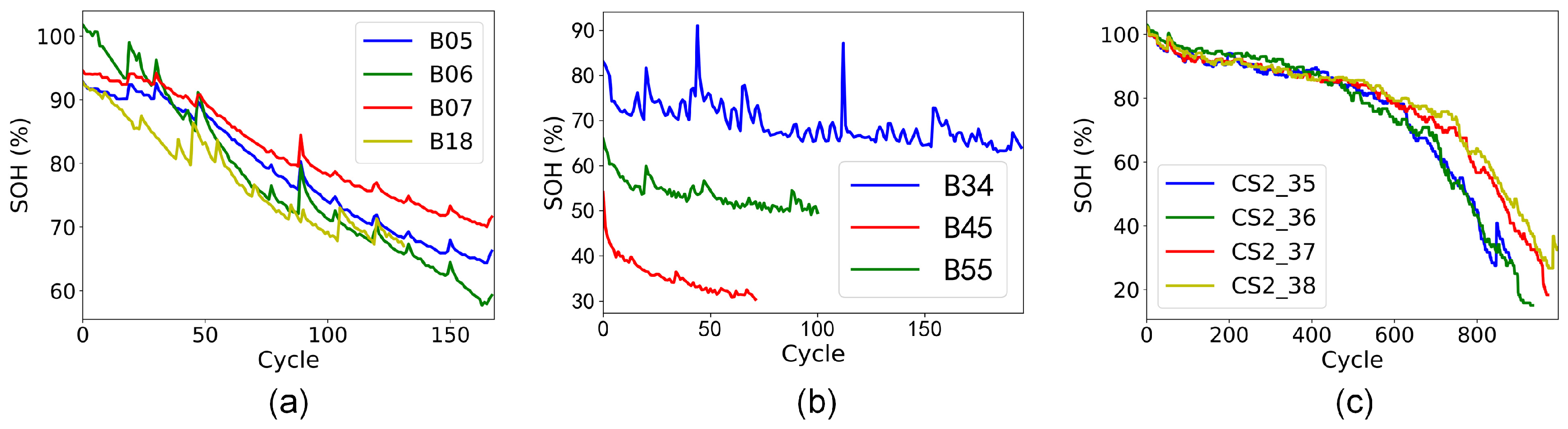
2.1. Battery Degradation Data Analysis
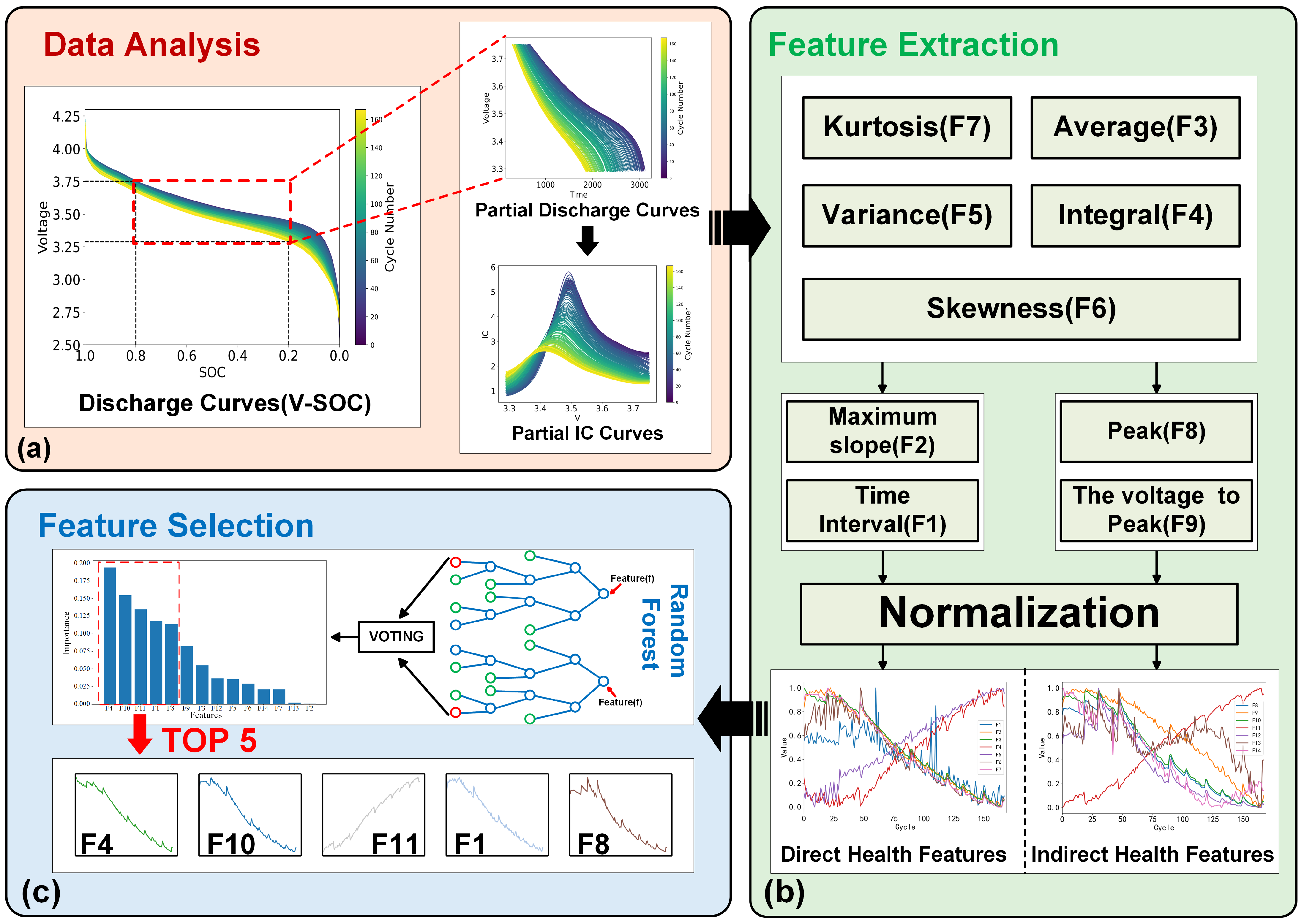
2.2. Health Feature Construction Based on Partial Discharge Curves
2.2.1. Feature Extraction Based on Voltage Curve
2.2.2. Feature Extraction Based on the IC Curve
2.3. Health Feature Analysis Based on Random Forest Regression
- (1)
- For the original data , the random forest regression model accuracy , represented here by the mean square error (MSE), is calculated as follows:where and are the estimated and actual values of SOH for the -th sample, respectively, and is the number of samples.
- (2)
- To reduce the chance error caused by randomly replacing features, the following steps are repeated times (with set to 5 in our experiments): replace the features and record the newly generated dataset as ; recalculate the model’s accuracy for the new dataset .
- (3)
- Calculate the feature importance for feature :
- (4)
- After obtaining the importance of all the features, the data is normalized to obtain the final importance as follows:
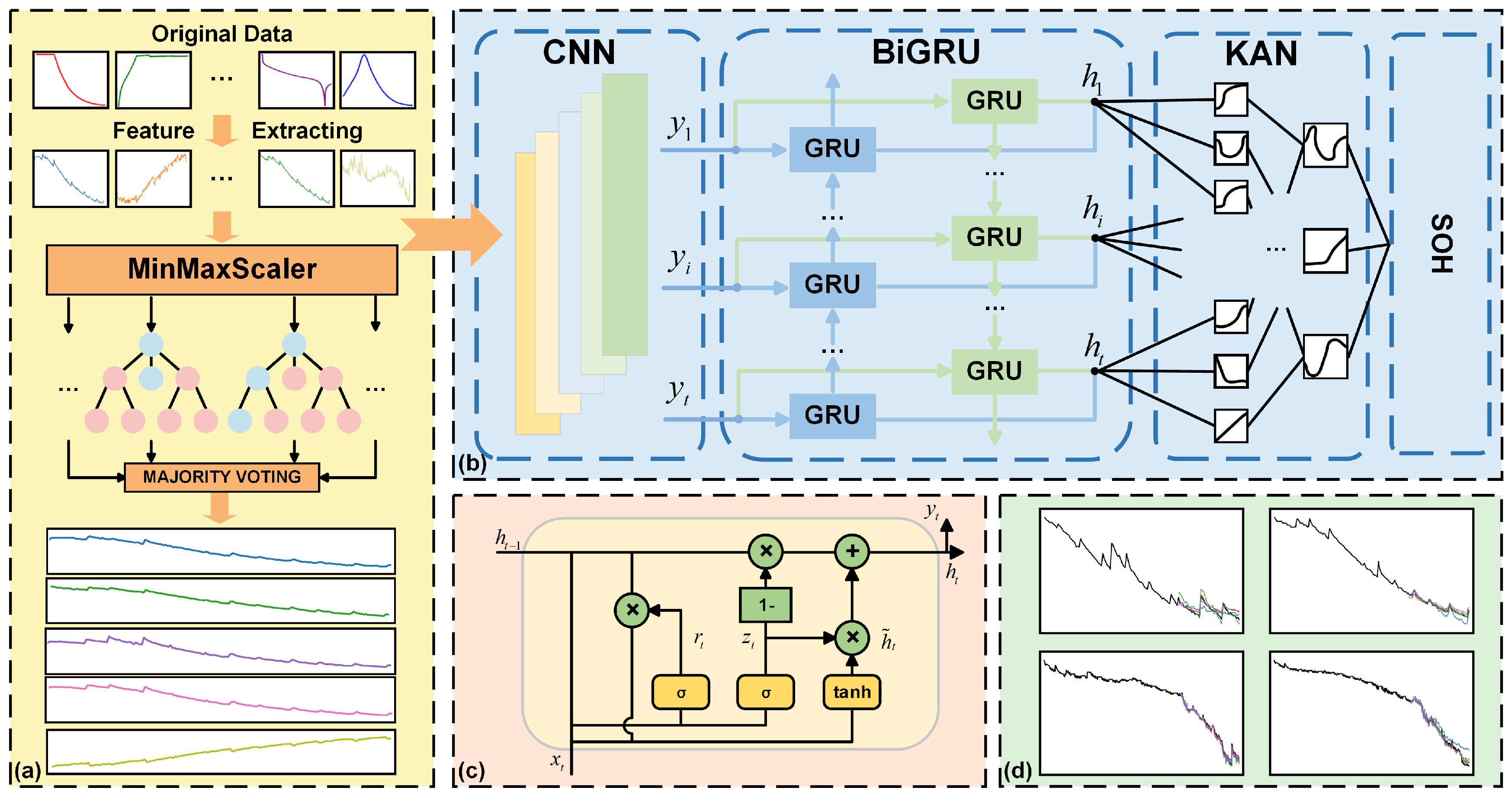
3. Method
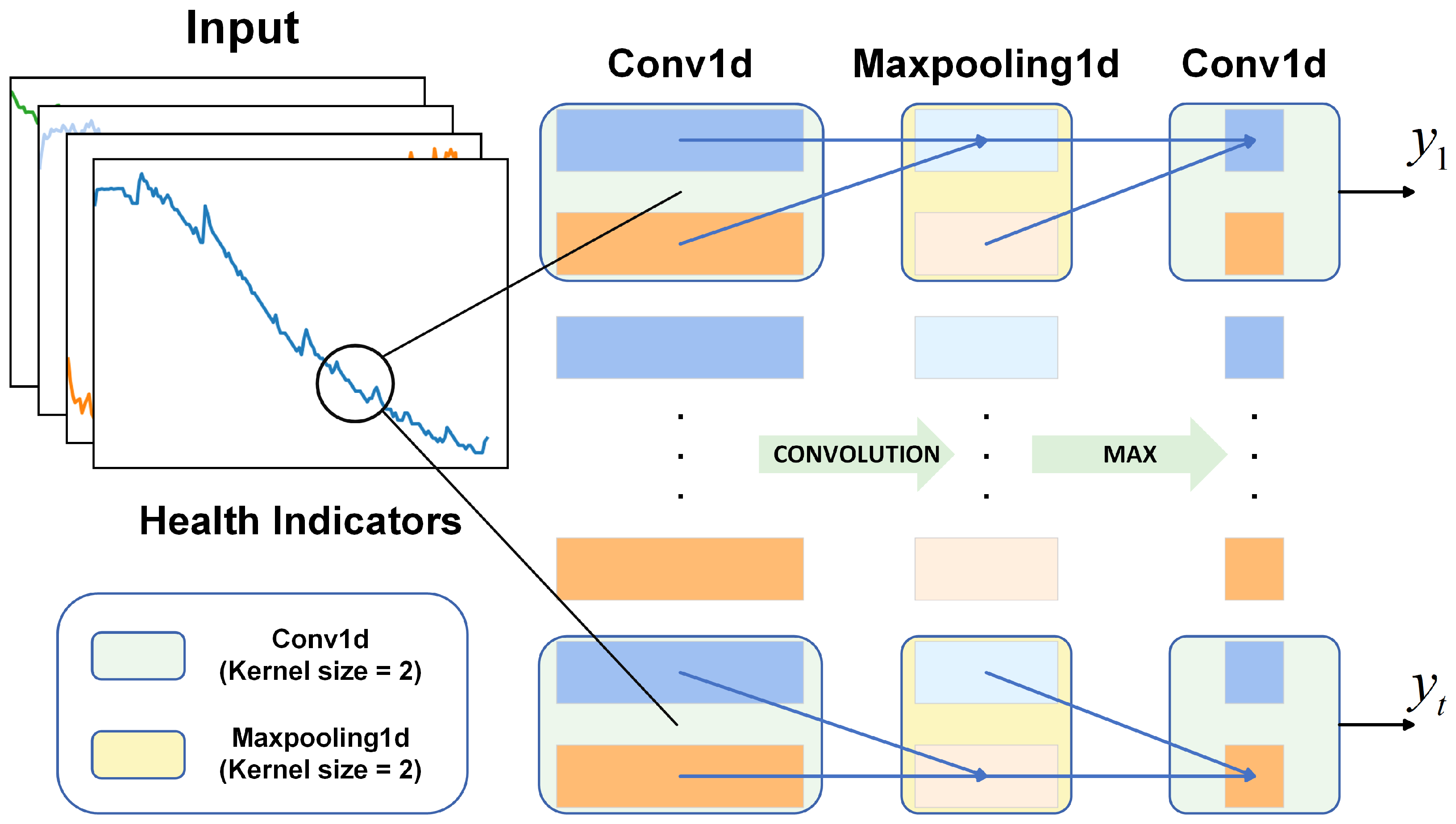
3.1. 1D-CNN
3.2. BiGRU
3.3. KAN
3.4. CGKAN
4. Experiments and Analysis
4.1. SOH Estimation Accuracy Experiment
4.2. SOH Estimation Based on Multiple Battery Aging Information
4.3. SOH Estimation Experiment Under Complex Operating Conditions
5. Conclusions
Author Contributions
Funding
Data Availability Statement
Conflicts of Interest
References
- Song, L.; Zhang, K.; Liang, T.; Han, X.; Zhang, Y. Intelligent State of Health Estimation for Lithium-Ion Battery Pack Based on Big Data Analysis. J. Energy Storage 2020, 32, 101836. [Google Scholar] [CrossRef]
- Hu, X.; Zhang, K.; Liu, K.; Lin, X.; Dey, S.; Onori, S. Advanced Fault Diagnosis for Lithium-Ion Battery Systems: A Review of Fault Mechanisms, Fault Features, and Diagnosis Procedures. IEEE Ind. Electron. Mag. 2020, 14, 65–91. [Google Scholar] [CrossRef]
- Sui, X. Robust State of Health Estimation for Lithium-Ion Batteries Using Machines Learning; Aalborg University: Aalborg, Denmark, 2021. [Google Scholar]
- Wu, J.; Cui, X.; Meng, J.; Peng, J.; Lin, M. Data-Driven Transfer-Stacking Based State of Health Estimation for Lithium-Ion Batteries. IEEE Trans. Ind. Electron. 2023, 71, 604–614. [Google Scholar] [CrossRef]
- Li, Q.; Li, D.; Zhao, K.; Wang, L.; Wang, K. State of Health Estimation of Lithium-Ion Battery Based on Improved Ant Lion Optimization and Support Vector Regression. J. Energy Storage 2022, 50, 104215. [Google Scholar] [CrossRef]
- Lyu, C.; Lai, Q.; Ge, T.; Yu, H.; Wang, L.; Ma, N. A Lead-Acid Battery’s Remaining Useful Life Prediction by Using Electrochemical Model in the Particle Filtering Framework. Energy 2017, 120, 975–984. [Google Scholar] [CrossRef]
- Hu, X.; Li, S.; Peng, H. A Comparative Study of Equivalent Circuit Models for Li-Ion Batteries. J. Power Sources 2012, 198, 359–367. [Google Scholar] [CrossRef]
- Wang, Y.; Tian, J.; Sun, Z.; Wang, L.; Xu, R.; Li, M.; Chen, Z. A Comprehensive Review of Battery Modeling and State Estimation Approaches for Advanced Battery Management Systems. Renew. Sustain. Energy Rev. 2020, 131, 110015. [Google Scholar] [CrossRef]
- Xiong, R.; Li, L.; Li, Z.; Yu, Q.; Mu, H. An Electrochemical Model Based Degradation State Identification Method of Lithium-Ion Battery for All-Climate Electric Vehicles Application. Appl. Energy 2018, 219, 264–275. [Google Scholar] [CrossRef]
- Deng, Z.; Hu, X.; Lin, X.; Xu, L.; Li, J.; Guo, W. A Reduced-Order Electrochemical Model for All-Solid-State Batteries. IEEE Trans. Transp. Electrif. 2020, 7, 464–473. [Google Scholar] [CrossRef]
- Galeotti, M.; Cinà, L.; Giammanco, C.; Cordiner, S.; Di Carlo, A. Performance Analysis and SOH (State of Health) Evaluation of Lithium Polymer Batteries through Electrochemical Impedance Spectroscopy. Energy 2015, 89, 678–686. [Google Scholar] [CrossRef]
- Hu, X.; Yuan, H.; Zou, C.; Li, Z.; Zhang, L. Co-Estimation of State of Charge and State of Health for Lithium-Ion Batteries Based on Fractional-Order Calculus. IEEE Trans. Veh. Technol. 2018, 67, 10319–10329. [Google Scholar] [CrossRef]
- Li, J.; Adewuyi, K.; Lotfi, N.; Landers, R.; Park, J. A Single Particle Model with Chemical/Mechanical Degradation Physics for Lithium Ion Battery State of Health (SOH) Estimation. Appl. Energy 2018, 212, 1178–1190. [Google Scholar] [CrossRef]
- Chen, S.-Z.; Liang, Z.; Yuan, H.; Yang, L.; Xu, F.; Zhang, Y. Li-Ion Battery State-of-Health Estimation Based on the Combination of Statistical and Geometric Features of the Constant-Voltage Charging Stage. J. Energy Storage 2023, 72, 108647. [Google Scholar] [CrossRef]
- Fezai, R.; Abodayeh, K.; Mansouri, M.; Nounou, H.; Nounou, M. Fault Diagnosis of Biological Systems Using Improved Machine Learning Technique. Int. J. Mach. Learn. Cybern. 2021, 12, 515–528. [Google Scholar] [CrossRef]
- Gou, B.; Xu, Y.; Feng, X. An Ensemble Learning-Based Data-Driven Method for Online State-of-Health Estimation of Lithium-Ion Batteries. IEEE Trans. Transp. Electrif. 2020, 7, 422–436. [Google Scholar] [CrossRef]
- Teng, J.-H.; Chen, R.-J.; Lee, P.-T.; Hsu, C.-W. Accurate and Efficient SOH Estimation for Retired Batteries. Energies 2023, 16, 1240. [Google Scholar] [CrossRef]
- Pan, H.; Lü, Z.; Wang, H.; Wei, H.; Chen, L. Novel Battery State-of-Health Online Estimation Method Using Multiple Health Indicators and an Extreme Learning Machine. Energy 2018, 160, 466–477. [Google Scholar] [CrossRef]
- Zhu, J.; Wang, Y.; Huang, Y.; Bhushan Gopaluni, R.; Cao, Y.; Heere, M.; Mühlbauer, M.J.; Mereacre, L.; Dai, H.; Liu, X.; et al. Data-Driven Capacity Estimation of Commercial Lithium-Ion Batteries from Voltage Relaxation. Nat. Commun. 2022, 13, 2261. [Google Scholar] [CrossRef]
- Weng, C.; Sun, J.; Peng, H. Model Parametrization and Adaptation Based on the Invariance of Support Vectors with Applications to Battery State-of-Health Monitoring. IEEE Trans. Veh. Technol. 2014, 64, 3908–3917. [Google Scholar] [CrossRef]
- Wang, Z.; Yuan, C.; Li, X. Lithium Battery State-of-Health Estimation via Differential Thermal Voltammetry with Gaussian Process Regression. IEEE Trans. Transp. Electrif. 2020, 7, 16–25. [Google Scholar] [CrossRef]
- Wu, M.; Zhong, Y.; Wu, J.; Wang, Y.; Wang, L. State of Health Estimation of the Lithium-Ion Power Battery Based on the Principal Component Analysis-Particle Swarm Optimization-Back Propagation Neural Network. Energy 2023, 283, 129061. [Google Scholar] [CrossRef]
- Yun, Z.; Qin, W.; Shi, W.; Ping, P. State-of-Health Prediction for Lithium-Ion Batteries Based on a Novel Hybrid Approach. Energies 2020, 13, 4858. [Google Scholar] [CrossRef]
- Yang, N.; Song, Z.; Hofmann, H.; Sun, J. Robust State of Health estimation of lithium-ion batteries using convolutional neural network and random forest. J. Energy Storage 2022, 48, 103857. [Google Scholar] [CrossRef]
- Zheng, Y.; Hu, J.; Chen, J.; Deng, H.; Hu, W. State of health estimation for lithium battery random charging process based on CNN-GRU method. Energy Rep. 2023, 9, 1–10. [Google Scholar] [CrossRef]
- Wang, X.; Hu, B.; Su, X.; Xu, L.; Zhu, D. State of Health estimation for lithium-ion batteries using Random Forest and Gated Recurrent Unit. J. Energy Storage 2024, 76, 109796. [Google Scholar] [CrossRef]
- Saha, B.; Goebel, K. Battery Data Set; NASA Prognostics Data Repository, NASA Ames Research Center: Moffett Field, CA, USA, 2007. Available online: https://www.nasa.gov/intelligent-systems-division/discovery-and-systems-health/pcoe/pcoe-data-set-repository/ (accessed on 10 February 2025).
- CALCE Battery Research Group of the University of Maryland. Battery Data Set. Available online: https://calce.umd.edu/battery-data (accessed on 10 February 2025).
- Goebel, K.; Saha, B.; Saxena, A.; Celaya, J.R.; Christophersen, J.P. Prognostics in Battery Health Management. IEEE Instrum. Meas. Mag. 2008, 11, 33–40. [Google Scholar] [CrossRef]
- He, W.; Williard, N.; Osterman, M.; Pecht, M. Prognostics of Lithium-Ion Batteries Based on Dempster–Shafer Theory and the Bayesian Monte Carlo Method. J. Power Sources 2011, 196, 10314–10321. [Google Scholar] [CrossRef]
- Jia, Q.-S.; Long, T. A Review on Charging Behavior of Electric Vehicles: Data, Model, and Control. Control Theory Technol. 2020, 18, 217–230. [Google Scholar] [CrossRef]
- Xu, J.; Liu, B.; Zhang, G.; Zhu, J. State-of-health Estimation for Lithium-ion Batteries Based on Partial Charging Segment and Stacking Model Fusion. Energy Sci. Eng. 2023, 11, 383–397. [Google Scholar] [CrossRef]
- Lin, M.; Wu, D.; Meng, J.; Wu, J.; Wu, H. A Multi-Feature-Based Multi-Model Fusion Method for State of Health Estimation of Lithium-Ion Batteries. J. Power Sources 2022, 518, 230774. [Google Scholar] [CrossRef]
- Zhi, Y.; Wang, H.; Wang, L. A State of Health Estimation Method for Electric Vehicle Li-Ion Batteries Using GA-PSO-SVR. Complex Intell. Syst. 2022, 8, 2167–2182. [Google Scholar] [CrossRef]
- Breiman, L. Random Forests. Mach. Learn. 2001, 45, 5–32. [Google Scholar] [CrossRef]
- Firsov, N.; Myasnikov, E.; Lobanov, V.; Khabibullin, R.; Kazanskiy, N.; Khonina, S.; Butt, M.A.; Nikonorov, A. HyperKAN: Kolmogorov–Arnold Networks Make Hyperspectral Image Classifiers Smarter. Sensors 2024, 24, 7683. [Google Scholar] [CrossRef]
- Livieris, I.E. C-KAN: A New Approach for Integrating Convolutional Layers with Kolmogorov–Arnold Networks for Time-Series Forecasting. Mathematics 2024, 12, 3022. [Google Scholar] [CrossRef]
- Kolmogorov, A.N. On the Representation of Continuous Functions of Several Variables by Superpositions of Continuous Functions of a Smaller Number of Variables; American Mathematical Society: Providence, RI, USA, 1961. [Google Scholar]
- Liu, Z.; Wang, Y.; Vaidya, S.; Ruehle, F.; Halverson, J.; Soljačić, M.; Hou, T.Y.; Tegmark, M. Kan: Kolmogorov-arnold networks. arXiv 2024, arXiv:2404.19756. [Google Scholar]


| Battery | °C | Charging (A) | Cutoff (V) | Discharging (A) | Cutoff (V) |
|---|---|---|---|---|---|
| B05, B06, B07, B18 | 24 | 1.5 | 4.2 | 2.0 | 2.7, 2.5, 2.2, 2.5 |
| B34, B45, B55 | 24, 4, 4 | 1.5 | 4.2 | 4.0, 1.0, 2.0 | 2.2, 2.0, 2.5 |
| CS2_35, CS2_36, CS2_37, CS2_38 | \ | 0.55 | 4.2 | 1.1 | 2.7 |
| No. | Starting Cycle | Method | MAE (%) | RMSE (%) | MAPE (%) |
|---|---|---|---|---|---|
| B05 | Cycle115 (70%) | CGKAN | 0.40 | 0.47 | 0.60 |
| CNN | 0.80 | 1.00 | 4.26 | ||
| BiGRU | 0.15 | 0.19 | 0.22 | ||
| CNN-BiGRU | 0.61 | 0.72 | 0.92 | ||
| B06 | Cycle115 (70%) | CGKAN | 0.78 | 1.01 | 1.26 |
| CNN | 0.88 | 1.10 | 1.42 | ||
| BiGRU | 0.97 | 1.14 | 1.57 | ||
| CNN-BiGRU | 1.12 | 1.46 | 1.88 | ||
| B07 | Cycle115 (70%) | CGKAN | 0.63 | 0.74 | 0.88 |
| CNN | 0.97 | 1.11 | 1.33 | ||
| BiGRU | 1.28 | 1.44 | 1.78 | ||
| CNN-BiGRU | 1.09 | 1.38 | 1.52 | ||
| B18 | Cycle90 (70%) | CGKAN | 0.66 | 0.85 | 0.96 |
| CNN | 0.98 | 1.20 | 1.41 | ||
| BiGRU | 0.81 | 1.02 | 1.15 | ||
| CNN-BiGRU | 0.89 | 1.06 | 1.29 | ||
| AVERAGE | 70% | CGKAN | 0.62 | 0.77 | 0.93 |
| CNN | 0.91 | 1.10 | 2.11 | ||
| BiGRU | 0.80 | 0.95 | 1.18 | ||
| CNN-BiGRU | 0.93 | 1.16 | 1.40 | ||
| B05 | Cycle80 (50%) | CGKAN | 0.60 | 0.68 | 0.87 |
| CNN | 2.42 | 2.64 | 3.43 | ||
| BiGRU | 0.68 | 0.81 | 0.99 | ||
| CNN-BiGRU | 2.42 | 3.04 | 3.58 | ||
| B18 | Cycle65 (50%) | CGKAN | 0.58 | 0.77 | 0.81 |
| CNN | 1.50 | 1.84 | 2.14 | ||
| BiGRU | 1.01 | 1.09 | 1.43 | ||
| CNN-BiGRU | 1.25 | 1.48 | 1.80 | ||
| AVERAGE | 50% | CGKAN | 0.59 | 0.73 | 0.84 |
| CNN | 1.96 | 2.24 | 2.79 | ||
| BiGRU | 0.85 | 0.95 | 1.21 | ||
| CNN-BiGRU | 1.84 | 2.26 | 2.69 |
| No. | Starting Cycle | Method | MAE (%) | RMSE (%) | MAPE (%) |
|---|---|---|---|---|---|
| CS2_35 | Cycle617 (70%) | CGKAN | 0.95 | 1.25 | 2.38 |
| CNN | 1.17 | 1.55 | 2.71 | ||
| BiGRU | 1.34 | 1.66 | 3.03 | ||
| CNN-BiGRU | 1.30 | 1.68 | 2.89 | ||
| CS2_36 | Cycle655 (70%) | CGKAN | 0.91 | 1.15 | 3.27 |
| CNN | 4.28 | 5.71 | 17.51 | ||
| BiGRU | 1.34 | 1.74 | 5.16 | ||
| CNN-BiGRU | 2.11 | 2.61 | 7.61 | ||
| CS2_37 | Cycle680 (70%) | CGKAN | 1.28 | 1.57 | 3.22 |
| CNN | 2.24 | 3.99 | 7.64 | ||
| BiGRU | 1.34 | 2.09 | 4.17 | ||
| CNN-BiGRU | 1.38 | 1.73 | 3.72 | ||
| CS2_38 | Cycle697 (70%) | CGKAN | 1.26 | 1.53 | 2.50 |
| CNN | 3.23 | 3.70 | 6.65 | ||
| BiGRU | 2.59 | 2.99 | 6.30 | ||
| CNN-BiGRU | 1.42 | 1.61 | 3.01 | ||
| AVERAGE | 70% | CGKAN | 1.10 | 1.38 | 2.84 |
| CNN | 2.73 | 3.74 | 8.63 | ||
| BiGRU | 1.65 | 2.12 | 4.67 | ||
| CNN-BiGRU | 1.55 | 1.91 | 4.31 | ||
| CS2_35 | Cycle441 (50%) | CGKAN | 1.33 | 1.99 | 3.06 |
| CNN | 2.24 | 2.95 | 4.65 | ||
| BiGRU | 2.20 | 2.49 | 4.43 | ||
| CNN-BiGRU | 1.72 | 2.66 | 4.09 | ||
| CS2_38 | Cycle498 (50%) | CGKAN | 2.03 | 2.64 | 4.58 |
| CNN | 2.68 | 4.00 | 6.44 | ||
| BiGRU | 3.34 | 2.66 | 6.01 | ||
| CNN-BiGRU | 3.19 | 4.50 | 7.63 | ||
| AVERAGE | 50% | CGKAN | 1.68 | 2.32 | 3.82 |
| CNN | 2.46 | 3.48 | 5.55 | ||
| BiGRU | 2.77 | 2.58 | 5.22 | ||
| CNN-BiGRU | 2.46 | 3.58 | 5.86 |
| No. | Method | RMSE (%) | Parameters (M) | Model Size (MB) | FLOPs (M) |
|---|---|---|---|---|---|
| B18 | CGKAN | 0.66 | 0.16 | 0.67 | 0.51 |
| SVM | 0.60 | - | 0.01 | - | |
| RNN | 1.04 | 0.03 | 0.11 | 0.15 | |
| LSTM | 1.14 | 0.08 | 0.32 | 0.43 | |
| CS2_38 | CGKAN | 1.26 | 0.16 | 0.67 | 0.51 |
| SVM | 1.34 | - | 0.01 | - | |
| RNN | 1.95 | 0.03 | 0.11 | 0.15 | |
| LSTM | 5.06 | 0.08 | 0.32 | 0.43 | |
| AVERAGE | CGKAN | 0.96 | 0.16 | 0.67 | 0.51 |
| SVM | 0.97 | - | 0.01 | - | |
| RNN | 1.50 | 0.03 | 0.11 | 0.15 | |
| LSTM | 3.10 | 0.08 | 0.32 | 0.43 |
| Training Data | Test Data | MAE (%) | RMSE (%) | MAPE (%) |
|---|---|---|---|---|
| B06+07+18 | B05 | 0.70 | 0.90 | 0.92 |
| B05+07+18 | B06 | 1.69 | 1.98 | 2.27 |
| B05+06+18 | B07 | 1.30 | 1.68 | 1.61 |
| B05+06+07 | B18 | 2.00 | 2.38 | 2.50 |
| CS2_36+37+38 | CS2_35 | 1.04 | 1.50 | 1.89 |
| CS2_35+37+38 | CS2_36 | 1.66 | 2.98 | 5.14 |
| CS2_35+36+38 | CS2_37 | 1.59 | 1.99 | 2.84 |
| CS2_35+36+37 | CS2_38 | 1.26 | 1.67 | 2.13 |
| No. | Starting Cycle | MAE (%) | RMSE (%) | MAPE (%) |
|---|---|---|---|---|
| B34 | Cycle135 (70%) | 0.74 | 0.96 | 1.11 |
| B45 | Cycle50 (70%) | 0.41 | 0.50 | 1.28 |
| B55 | Cycle70 (70%) | 0.61 | 0.75 | 1.19 |
| CS2_3 | Cycle70 (70%) | 1.45 | 1.77 | 1.93 |
| AVERAGE | 70% | 0.80 | 0.99 | 1.37 |
| B34 | Cycle100 (50%) | 0.86 | 1.39 | 1.26 |
Disclaimer/Publisher’s Note: The statements, opinions and data contained in all publications are solely those of the individual author(s) and contributor(s) and not of MDPI and/or the editor(s). MDPI and/or the editor(s) disclaim responsibility for any injury to people or property resulting from any ideas, methods, instructions or products referred to in the content. |
© 2025 by the authors. Licensee MDPI, Basel, Switzerland. This article is an open access article distributed under the terms and conditions of the Creative Commons Attribution (CC BY) license (https://creativecommons.org/licenses/by/4.0/).
Share and Cite
He, S.; Qin, W.; Yun, Z.; Wu, C.; Sun, C. SOH Estimation Method for Lithium-Ion Batteries Using Partial Discharge Curves Based on CGKAN. Batteries 2025, 11, 167. https://doi.org/10.3390/batteries11050167
He S, Qin W, Yun Z, Wu C, Sun C. SOH Estimation Method for Lithium-Ion Batteries Using Partial Discharge Curves Based on CGKAN. Batteries. 2025; 11(5):167. https://doi.org/10.3390/batteries11050167
Chicago/Turabian StyleHe, Shengfeng, Wenhu Qin, Zhonghua Yun, Chao Wu, and Chongbin Sun. 2025. "SOH Estimation Method for Lithium-Ion Batteries Using Partial Discharge Curves Based on CGKAN" Batteries 11, no. 5: 167. https://doi.org/10.3390/batteries11050167
APA StyleHe, S., Qin, W., Yun, Z., Wu, C., & Sun, C. (2025). SOH Estimation Method for Lithium-Ion Batteries Using Partial Discharge Curves Based on CGKAN. Batteries, 11(5), 167. https://doi.org/10.3390/batteries11050167