Abstract
There are many challenges in incorporating the attenuation cost of energy storage into the optimization of microgrid operations due to the randomness of renewable energy supply, the high cost of controlled power generation, and the complexity associated with calculating the cost of battery attenuation. Therefore, this paper proposes a microgrid energy management scheme considering the attenuation cost of energy storage. This scheme analyzes the power generation mode and uncertainty factors of distributed generators in detail. The influence of charge and discharge depth on the cycle life and residual value of the energy storage system was analyzed, and the energy storage attenuation cost model was established. Finally, considering the cost of power generation, environmental treatment, and the deterioration cost of energy storage systems, the objective function of the comprehensive operation cost of microgrids is formulated. The improved sine cosine algorithm (SCA) is used to simulate the energy output optimization of various distributed generators in the microgrid. The results show that the algorithm can effectively reduce the comprehensive operation cost of microgrids and improve their energy utilization efficiency, which proves the practical significance and reference value of the method for microgrid energy management.
1. Introduction
Against the backdrop of rapid development in renewable energy, traditional power systems are continuously optimizing their energy structures by introducing new clean energy sources and integrating them into the grid. Nowadays, the distributed generation of renewable energy, such as wind and solar power, is widely regarded as an environmentally and economically beneficial solution for future smart grids. The integration of clean energy into distributed power systems effectively enhances energy efficiency and the penetration rate of renewable energy. This significantly reduces the emissions of carbon dioxide and other harmful gases associated with traditional fossil fuel-based power generation, thereby helping to mitigate climate change and improve environmental quality. With the development and application of clean energy technologies, it is foreseeable that clean energy generation will become an integral part of the global energy system in the future.
Simultaneously, the introduction of clean energy is driving the development of microgrids. Microgrids integrate traditional generators with new energy sources to provide power services to users in a decentralized manner [1]. With the ability to generate power independently and the flexibility to connect or disconnect from the utility grid, microgrids offer new avenues for the utilization of new energy sources. Microgrids effectively alleviate the supply pressure and environmental pollution of traditional power units. Moreover, during utility grid failures, microgrid systems can independently supply power to maintain normal operation. Compared to traditional power systems, microgrids have stronger local consumption capabilities. By managing the output of distributed power sources and scheduling energy usage rationally [2], clean energy can be utilized more effectively.
Microgrids typically consist of various distributed power sources, energy storage devices, energy conversion equipment, loads, and various protective devices, forming a power supply system capable of achieving internal power balance [3]. Distributed power sources generally consist of both renewable and traditional energy sources, which complement each other to support load balancing. Energy storage devices effectively store electricity from renewable sources and release it when needed to meet grid demands or provide backup power. Common energy storage devices include battery energy storage systems (such as lithium ion batteries, sodium sulfur batteries, etc.), pumped hydro storage, and compressed air energy storage. These devices not only improve the stability and reliability of microgrids but also help regulate load and balance differences between supply and demand in the power system, thereby achieving more effective grid management.
Although microgrids are considered crucial components of future power systems, they still encounter various challenges in practical applications. The main issues facing microgrid systems currently include:
(1) Reliability: The generation of renewable energy sources in the system is greatly affected by weather fluctuations, leading to unstable power generation in microgrid systems.
(2) Power Quality: Due to the inclusion of various distributed energy sources and loads, issues related to power quality within the microgrid (such as voltage fluctuations and harmonics) may affect power supply quality and equipment lifespan.
(3) Energy Management: Microgrids require the effective management of multiple distributed energy sources, including solar, wind, and batteries, to ensure stable power supply. This involves complex energy scheduling and optimization problems.
(4) Economic: The construction and operation costs of microgrids are relatively high, especially considering the constant technological updates and intense market competition. Thus, reducing costs and achieving economic feasibility are key issues.
Addressing the above problems, this paper proposes a series of solutions. To ensure the reliability of microgrid system operation, energy storage systems, diesel generators, and grid power are introduced to meet electricity loads during fluctuations in renewable energy generation, thus ensuring system stability. To tackle power quality, operational constraints are set for various distributed energy sources to control their output power limits, preventing drastic energy fluctuations that could affect equipment lifespan. As for energy management and economic issues, this paper introduces metaheuristic algorithms for optimizing microgrid energy management and overall costs.
The rapid solving capability and precise calculation ability of metaheuristic algorithms provide feasible solutions for optimizing microgrid energy management, sparking a surge in research on microgrid operation optimization. However, previous optimization processes often only considered economic and environmental pollution factors, neglecting the degradation costs of energy storage systems. In reality, in microgrid systems, due to the uncertainty of wind and solar power generation, energy storage systems undergo frequent charging and discharging, accelerating battery degradation. Thus, strategically planning the timing and depth of battery charging and discharging to reduce storage degradation costs is crucial for overall energy scheduling in microgrids. This paper considers the degradation costs of energy storage systems as a key element of microgrid system operating costs, together with economic costs and environmental costs, forming the comprehensive operating costs of microgrids, and uses an improved SCA to optimize them.
The main contributions of this paper are as follows:
(1) Establishing a microgrid energy storage system represented by lithium batteries, constructing degradation costs, and integrating them into the total operation costs of microgrids;
(2) Improving the SCA using two strategies: circle chaos mapping and Levy flight, and demonstrating the effectiveness of the improved algorithm through test functions;
(3) Using the improved SCA to simulate and optimize the operating costs of microgrid systems, demonstrating that the improved algorithm effectively reduces the overall operating costs of microgrids.
The structure of the article is as follows: Section 2 reviews previous work, Section 3 and Section 4 introduce the degradation model of energy storage and the design of the comprehensive operating cost function of microgrids, Section 5 introduces the improved SCA, and Section 6 and Section 7 present the experiments and conclusions of this paper, respectively.
2. Related Work
Wind power generation, as a significant form of renewable energy, holds a crucial position in today’s energy sector, and wind energy has now become one of the primary sources of global electricity supply [4]. Wind power generation refers to the process of converting wind energy into mechanical energy and then into electrical energy through wind turbines. Wind power generation utilizes the wind to drive the rotation of turbine blades, which are connected to the generator rotor. The rotating rotor induces electrical current within the generator through magnetic field induction, thereby generating electrical energy. In recent years, the manufacturing cost of wind turbines has continuously decreased, and they are commonly equipped with smart sensors, resulting in improved operational efficiency and further reduction in usage costs.
Photovoltaic (PV) power generation is the process of directly converting sunlight radiation into electrical energy and is an important form of renewable energy. The core component of photovoltaic power generation is the solar panel, which consists of multiple solar cells. These cells can convert photons from sunlight into electrons, thus generating electrical current. Photovoltaic technology features renewable, non-polluting, and low-noise characteristics, playing a significant role in sustainable development and climate change mitigation [5]. With continuous technological advancements and cost reductions, photovoltaic power generation has been widely deployed globally.
Wind power and photovoltaic power, as major clean energy technologies, play a critical role in addressing climate change and energy security challenges. Their generation processes involve minimal direct greenhouse gas emissions, contributing to improved environmental quality and exhibiting significant renewability. Additionally, their relatively low operation and maintenance costs contribute to enhanced economic benefits. However, wind and photovoltaic power generation are significantly influenced by weather factors, resulting in substantial output power fluctuations within microgrids, necessitating coordinated operation with other generation equipment.
Duan, YZ [6] proposed a fully distributed algorithm that does not rely on the initialization process to solve the dynamic scheduling problem of hybrid microgrids. The optimal solution satisfies the supply and demand constraints and the constraints of unequal production capacity at each time limit. Dey, B et al. [7] proposed a demand response (DR) model to maximize the advantages of microgrids, taking into account various aspects of utility and elasticity, as well as customer behavior. The optimization model can reduce the overall cost of the microgrid system. Zhao, ZL [8] proposed a new autonomous multi-microgrid intraday robust energy management framework based on the distributed dynamic management model predictive control (DD-TMPC) method. The proposed strategy can dynamically capture the safe operating range of the microgrid system based on set theory. Wongdet, P [9] proposed a capacity optimization method and cost analysis considering the life cycle of a battery energy storage system (BESS), which is conducive to reducing the total cost. Hemmati, M [10] proposed a new energy management method for MMG networks in the presence of battery storage, renewable energy, and demand response (DR) plans. The uncertainty associated with the load and power output of wind and solar energy is handled by adopting the chance constrained programming (CCP) optimization framework in the MMG energy management model. Ref. [11] investigated the smart control problem of autonomous microgrids to ensure voltage safety and maximize economic and environmental benefits. Ref. [12] aimed to minimize total investment costs and technological factors and explored the design problem of microgrids composed of various types of distributed energy sources using the movable damping wave algorithm. Ref. [13] focused on the energy management of microgrid systems in islanded mode, considering demand forecasting, and utilized the strawberry optimization algorithm for optimized scheduling. Dong Haiyan [14] optimized the charging and discharging states of distributed energy sources in microgrids over multiple time ranges based on seasonal differences, aiming to achieve low carbon emissions under the low-carbon operation mode of microgrids. Wang et al. [15] proposed a mixed-integer second-order cone optimization problem and demonstrated the performance optimization of the integrated energy system for fault recovery.
The aforementioned studies in microgrid optimization scheduling did not take into account the impact of battery degradation factors on costs. Unlike generation resources, the short-term scheduling of energy storage systems (ESSs) significantly affects their long-term lifespan; for instance, frequent charging and discharging can greatly reduce battery life. On the other hand, the conflict between cost and benefit further complicates the energy management problem of microgrids. Increasing ESS capacity can provide greater operational reserves, making microgrid operations smoother, but at the cost of additional capital investment [15]. Additionally, most microgrid optimization scheduling problems use intelligent search algorithms for solutions; however, basic intelligent search algorithms suffer from slow convergence, weak global search capability, and susceptibility to local optima, necessitating improvements to enhance algorithm performance.
This paper incorporates battery degradation costs into the overall operating costs of microgrids, considering the depth of charge and discharge of batteries, the number of charge and discharge cycles, and cost losses during usage, and utilizes an improved SCA to optimize microgrid operating costs.
3. Energy Storage Degradation
The degradation of energy storage systems (ESSs) is crucial for analyzing and evaluating the economic operation of microgrids [16]. In order to accurately simulate the cost characteristics of microgrid energy management, this section discusses the structure of microgrids and the degradation costs of ESSs.
3.1. Microgrid Structure
Microgrid systems are complex and typically composed of distributed energy sources, energy storage devices, and loads [17]. Distributed energy sources are divided into controllable and uncontrollable categories. Uncontrollable distributed energy sources usually include renewable energy generation devices such as wind turbines and photovoltaic generators, while controllable distributed energy sources include micro gas turbines, diesel generators, and gas boilers. The variety of distributed energy sources in microgrids, each with its own operational characteristics, significantly increases the complexity of microgrid scheduling [18].
There is a classic microgrid in Figure 1 that includes wind power generation, photovoltaic power generation, diesel generators, energy storage batteries, and electricity procurement from the utility grid. This configuration involves multiple sources of electricity and a combination of diverse power equipment working in unison to ensure stable load operation.
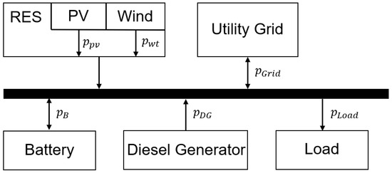
Figure 1.
Microgrid structure.
The characteristics of the mixed generation are reflected in the differences among various devices in terms of power density, energy density, lifespan, and cost. Batteries have high energy density and can store large amounts of electrical energy; diesel generators have high power density and can respond quickly to charging events. The combined characteristics of different power generation ends support the stable operation of microgrids.
At the same time, when interacting with the utility grid, microgrids can transmit the electricity they generate to the utility grid, reducing energy consumption. When the electricity generation of the microgrid is insufficient, the utility grid can also provide necessary electricity support. Microgrids can flexibly decide whether to sell or buy electricity from the utility grid based on their own electricity generation and load demand. Additionally, various means such as peak shaving and energy storage can be used to optimize electricity scheduling. During the interaction between microgrids and the utility grid, it is necessary to ensure stable and safe electricity quality and monitor and control electricity to prevent problems such as voltage fluctuations and momentary blackouts.
3.2. Factors Affecting Battery Life
Battery degradation mainly manifests in two aspects: cycle life, which reflects the total number of cycles that a battery unit can achieve, and capacity wear of battery units [19]. Cycle conditions, such as the frequency of charge–discharge cycles, charge–discharge rates, and maintenance schedules, have a significant impact on battery life. Battery life may accelerate degradation under unreasonable cycle conditions [20]. In addition to cycle conditions, state parameters also play an important role in battery life. Overcharging or undercharging states of charge (SOCs) can severely affect the charge–discharge performance of batteries. Temperature can also have adverse effects, especially under high-temperature conditions, where the degradation process of batteries may accelerate. In practical applications, a temperature controller is typically included in battery management systems. Therefore, we can assume that battery degradation caused by temperature factors can be ignored.
Furthermore, charge–discharge rates also affect battery life, but as long as the current does not exceed the limits specified by the manufacturer’s specifications, it should not be considered a long-term impact; hence, it is not considered in this paper.
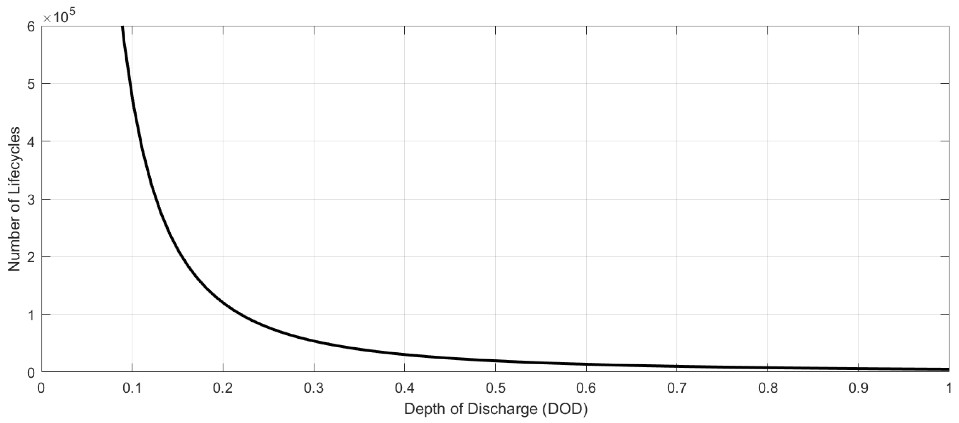
Therefore, the primary determinants of battery life are the actual full capacity and depth of discharge (DOD). Depending on different cycling events, there are typically two ways to define DOD. The first definition refers to the output energy at full capacity (100% SOC), while the second definition refers to a complete cycle composed of one charge–discharge event [21]. In this paper, we define DOD as the ratio of the energy change in one charge or discharge event to the energy at full battery capacity. Simultaneously, we define the actual full capacity of the battery as the energy that can be stored at 100% SOC. It should be noted that a cycle event is counted whenever the operating mode (charging and discharging) switches to the opposite side. The relationship between the number of battery cycles and DOD is illustrated in Figure 2. The fit of battery life is optimal when DOD = [22]:
where are curve fitting coefficients, is battery life, and is the depth of charge. The number of cycles in the battery’s lifespan decreases with an increase in DOD. Without a loss of generality, this expression is also applicable to batteries of different parameter types. Standards for battery life are typically determined according to manufacturing specifications; however, it should be noted that all charge–discharge cycles in standard data are conducted under the assumption of constant depth of discharge (DOD). However, in practical operations, the assumption of constant DOD is evidently unrealistic. Estimating battery degradation costs using the above information would introduce significant errors; hence, there is a need to further consider expressions for battery life under actual operating conditions and provide more accurate assessments of battery life.
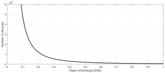
Figure 2.
Relationship between battery life cycle and DOD.
3.3. Battery Degradation Cost Model
To make the battery degradation cost model more practical, it is reasonable to assume that empirical data on lifespan are sufficiently accurate to estimate long-term degradation effects, meaning that the impact of each charge–discharge cycle event on lifespan is independent of historical charge–discharge curves. At the same time, this paper assumes that the degradation cost of each charge and discharge cycle event at different SOC levels is the same under the same DOD level [23].
The battery degradation cost model represents the direct depreciation of its actual capacity and lifespan. Considering a charging event starting at time t, with the average power during a time interval ∆t denoted as , the depth of charge over this time interval can be expressed as:
The actual capacity at time t is denoted as . The efficiency coefficients of charging and discharging, and , respectively, are defined. The average degradation cost per unit energy can be expressed as [24]:
This term refers to the average degradation cost of each charging and discharging event of DOD = , where represents the cost of battery replacement. Therefore, we can obtain the degradation cost of the battery corresponding to this discharge event by simply multiplying the energy output of the battery:
As the battery degrades, its health status also changes. This article defines the battery health status (SOH), where is the rated capacity of the battery:
After a complete cycle event, the actual capacity of the battery at t + ∆t is depreciated proportionally. At the same time, the health status of the battery will also affect the actual capacity. A lower SOH will accelerate battery decay. The formula for the actual capacity change of the battery is as follows, where is the capacity decay acceleration factor:
Of particular concern is that prolonged operation at an excessively high or low SOC can lead to increased internal impedance of the battery and electrolyte decomposition, thereby resulting in capacity loss and power attenuation. However, it is worth emphasizing that such degradation is relatively negligible in the short term compared to degradation caused by long-term charge–discharge events.
4. Microgrid Energy Management
This section focuses on the economic costs, environmental management costs, and storage degradation costs of microgrids, establishing a comprehensive cost function for microgrid operation, laying the foundation for subsequent energy management analysis. Simultaneously, it analyzes the specific operational characteristics of various distributed energy resources in microgrids and establishes operational constraints for distributed energy resources to ensure the reliability and stability of system operation.
4.1. Objective Function
This paper adopts the comprehensive operation cost of microgrids as the objective optimization function. Under the condition of ensuring the balance between electricity supply and demand in the microgrid, it not only considers operating costs and environmental benefits but also incorporates battery degradation costs as a long-term influencing factor into the consideration of comprehensive costs. It establishes the objective function for minimizing comprehensive operation costs, as follows:
where represents the minimum comprehensive operation cost of the microgrid system, denotes the generation cost of diesel generators, represents the battery degradation cost, signifies the cost of using grid electricity, and represents the cost required for environmental governance of the system. The following is a detailed analysis of the generation costs of various distributed energy sources.
4.1.1. Diesel Generator Power Generation Cost
In microgrid systems, diesel generators play a crucial role in maintaining supply–demand balance. With a lengthy developmental history, diesel generators have reached a considerable level of technical maturity and find extensive application as conventional power sources capable of swift startup and rapid shutdown in emergencies. They are characterized by their ability to generate stable electricity, exhibiting resilience to external influences and boasting high reliability. However, they incur high operational costs due to continuous fuel supply requirements, and the combustion of fuel leads to the emission of pollutants.
The relationship between diesel generator fuel costs and power output is described by the following equation, where α, β, and γ are constants, represents the output power of the diesel generator, and denotes the generator’s operating cost:
4.1.2. Battery Degradation Cost
The uncertainty and variability inherent in renewable energy generation pose challenges to the reliability and security of the power supply in microgrid systems. Energy storage systems, widely employed in microgrids, offer solutions for load balancing and energy regulation [25]. These systems possess the capability to dynamically absorb and release energy, enabling bidirectional energy control within specific time frames. When excess electricity is generated from wind and solar sources, energy storage systems can store surplus energy while meeting load demands. Conversely, when renewable energy generation falls short, these systems can provide power support to the microgrid.
Energy storage systems are primarily classified into three categories: chemical energy storage, physical energy storage, and electromagnetic energy storage. Physical energy storage encompasses forms such as flywheels, pumped hydro, and compressed air. Electromagnetic energy storage includes superconducting magnetic energy and supercapacitor energy storage, among others. Chemical energy storage encompasses technologies such as lead acid batteries, lithium ion batteries, flow batteries, and sodium sulfur batteries. Among these, lithium ion batteries, due to their relatively low cost and mature technology, have found widespread application in power systems. This paper focuses on the analysis of energy storage systems represented by lithium ion batteries. In Section 3.3 of this paper, the degradation cost of battery cycling events has been provided, considering charge–discharge efficiency. The energy variation equation of the battery over discrete time is given as:
Due to the fact that the degradation cost of the battery within each time interval can only be determined after the end of the charging or discharging event, it is necessary to specify the power flow direction of the battery. To address this, we first represent g(t) as an auxiliary binary variable, indicating the state transition of charging or discharging events between two consecutive time intervals:
represents the cumulative energy in kilowatt-hours (kWh) before the change of cycling events. Correspondingly, the cumulative energy can be expressed as:
Therefore, the degradation cost of the battery over consecutive time intervals can be expressed in terms of the state transition signal g(t) and the cumulative energy :
4.1.3. Utility Grid Power Generation Cost
The cost of grid electricity generation can be represented as follows:
The cost of utility grid generation at time t, denoted by , is influenced by the power output from the grid. In this paper, the utility grid is priced based on time-of-use (TOU) tariffs, which are divided into off-peak, standard, and peak periods. The fluctuation of electricity prices is also a significant parameter affecting the optimization of .
4.1.4. Environmental Governance Cost
In the optimization scheduling of microgrids, traditional models only consider economic costs while disregarding environmental considerations [26]. To better achieve the scheduling objectives of microgrid systems, it is imperative to comprehensively consider environmental factors. In this context, this paper precisely quantifies the pollutants generated by various types of generation units to achieve the goal of pollution reduction.
In the microgrid system studied in this paper, only photovoltaic and wind power generation can achieve zero emissions of pollutants. Other power generation devices release a certain amount of pollutants during the generation process. In this study, environmental costs are defined as the expenses required to mitigate the harmful gases produced by microgrid systems. These harmful gases include , , , , etc. The cost of pollutant treatment is expressed as follows:
where and are the emission coefficients of the i-th type of pollutants from the public power grid and the diesel generator, respectively; is the output power of the diesel generator; is the output power of the utility grid; is the treatment cost of the i-th type of pollutant.
4.2. System Restrictions
In the operation of microgrids, ensuring the satisfaction of load balance constraints is crucial. Load balance refers to the matching and equilibrium between the power output of various electrical components (such as generators, storage devices, renewable energy generation units, etc.) within the microgrid system and the load demand. At any given moment, the microgrid must maintain a balance between power supply and demand to ensure the stable operation of the power system. The power balance equation in this paper can be expressed as:
where represent the output power of the photovoltaic and wind turbines at time t, denotes the electrical load, and denotes the power output from the utility grid.
The inequality constraints include power limits for the grid, battery, and diesel generators, as well as capacity limits for the battery, expressed as follows:
, , , , , and represent the upper and lower limits of power generation for the grid, battery, and diesel generator, respectively. represent the upper and lower limits of the energy storage capacity.
5. Solving Optimization Problems Based on CLSCA
In addressing optimization problems in microgrids, metaheuristic algorithms are widely applied due to their strong dimensional handling capability and fast convergence speed. Among the plethora of metaheuristic algorithms, the SCA stands out for its advantages such as fewer parameters, simplicity in structure, and relatively fast convergence speed, demonstrating excellent performance in solving practical problems. This algorithm targets the oscillatory and periodic nature of sine and cosine functions as the design objective of its implementation operators, seeking optimal solutions through search and iteration [27].
While the SCA absorbs some advantages of traditional intelligent optimization algorithms in its iterative strategy, it still suffers from drawbacks such as slow convergence of the initial population and susceptibility to local optima, suggesting potential for improvement. In this study, we employ two strategies, circle chaotic mapping and Levy flight, to enhance the original SCA, aiming to achieve better performance in solving real-world problems.
5.1. Sine Cosine Algorithm
The sine cosine algorithm consists primarily of three steps: initialization, update, and selection. In the initialization phase, a set of initial individuals is generated based on a random algorithm, where each individual represents a solution in the search space. In the update phase, the iteration strategy of the SCA is categorized into two steps: global exploration and local exploitation. In global exploration, significant random fluctuations are applied to the solutions in the current population to explore unknown regions of the solution space. In local exploitation, weak random perturbations are applied to thoroughly search the neighborhood of the current solutions. Finally, in the selection phase, individuals with superior fitness values are selected for the next iteration through fitness comparison.
The SCA utilizes the periodic oscillations of sine and cosine functions to construct iteration equations that realize the functionalities of global exploration and local exploitation. These concise update equations impose perturbations and update the solution set. Specifically, the iteration equations are divided into two types: sine iteration or cosine iteration equations.
where , , , and are random numbers between 0 and 1; represents the fittest individual from the previous iteration.
5.2. Circle Chaos Map
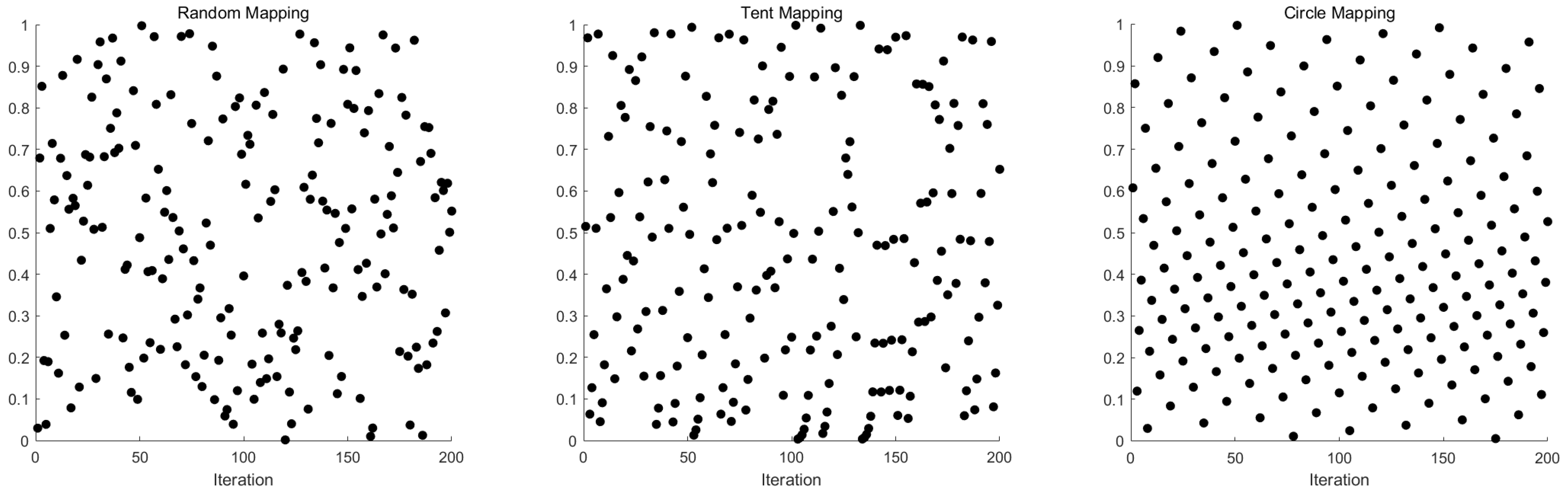
The SCA adopts a random generation of initial populations. Although convenient, this approach may lead to uneven population distribution and overall lower quality, resulting in instability in the early stages of algorithm execution. To address these issues, chaotic models are commonly employed during population generation to improve population quality. Currently used chaotic mappings include tent mapping, logistic mapping, and Chebyshev mapping [28]. Both Chebyshev and logistic mappings represent typical chaotic systems, where the mapping points exhibit high values at the ends and low values in the middle, causing uneven distribution, thereby affecting the algorithm’s search efficiency.
Compared to the dense distribution of boundary values in the logistic mapping range, tent chaotic mapping possesses both uniform probability density and good characteristics. Therefore, initializing populations using tent mapping can generate a more uniformly random distribution. However, tent mapping exhibits unstable periodic points in certain intervals. Meanwhile, circle mapping shares similar uniformity with tent mapping but offers a more balanced distribution at the ends of intervals [29]. The formula for calculating circle chaotic mapping is as follows:
This paper selects the circle mapping, which exhibits a more uniform distribution and greater stability, to enhance the SCA. This enhancement aims to increase individual diversity, thus accelerating the convergence speed of the algorithm. It facilitates better exploration of the solution space, improves stability, and achieves higher convergence accuracy. The distribution of random mapping, tent chaotic mapping, and circle mapping is illustrated in Figure 3 below:
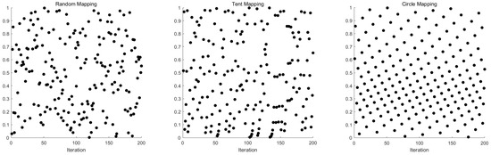
Figure 3.
Three random mappings.
5.3. Levy Flight
The Levy distribution is a probability distribution model proposed by the renowned French mathematician Paul Levy. It can be utilized to describe the flight trajectories of flying animals in nature, providing crucial insights for scientific research [30]. Levy flight represents a highly scalable stochastic process, enabling movements spanning multiple distances, thereby significantly expanding the search domain and enhancing the global search capabilities of algorithms. The Levy distribution is defined as follows:
The Levy distribution with parameter β is denoted as Levy(β), representing a random variable following this distribution. Levy(β) is defined by Equation (20), where u and v are normally distributed, and β is set to 1.5. The updated formula for SCA position, incorporating Levy flight trajectories, is presented as follows:
The pseudo-code of the improved algorithm is as follows (see Algorithm 1):
| Algorithm 1 The pseudo-code of the CLSCA |
| Initialize the population (i = 1, 2, …, N) with circle chaos mapping Calculate the fitness values of the initial search individuals while t< G Update rand1 for i = 1: N for j = 1:d Calculate the parameters rand2, rand3 and rand4 Update the positions of the search agents by Equation (19) End j Perform Lévy flight operator using Equation (22) to generate a candidate search agent Update the Amend the position of the current search individual based on lb and ub End i Return the best solution obtained so far as the global optimum |
5.4. Performance Testing
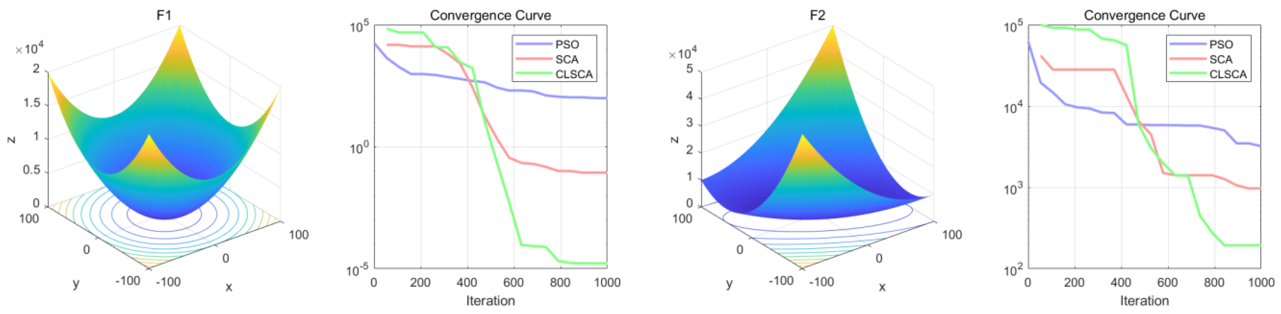
To validate the performance of the CLSCA, this study conducts tests using the benchmark functions from CEC2005. Four test functions are selected, comprising two unimodal functions and two multimodal functions. A comparison is made with classical PSO and the SCA to demonstrate the feasibility and effectiveness of CLSCA optimization. The unimodal functions assess the convergence speed and accuracy of the optimization algorithm, while the multimodal functions evaluate the global search capability. The test functions used are shown in Table 1:

Table 1.
Benchmark Functions.
All tested algorithms were iterated one thousand times with an initial population size set to 30. To mitigate experimental errors, each algorithm underwent 100 simulations to compute both the minimum and average values.
The objective space and convergence curves for unimodal functions are depicted in Figure 4:

Figure 4.
Unimodal function graph and convergence curve.
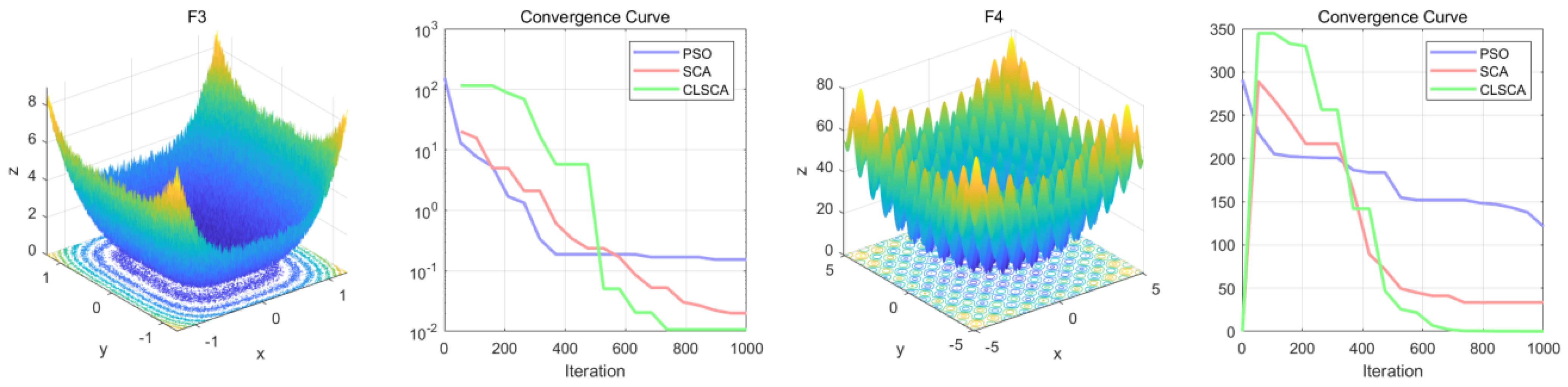
The target space diagram and convergence curve diagram of the multi-peak function are shown in Figure 5:
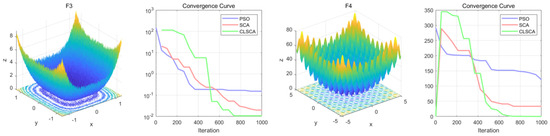
Figure 5.
Multimodal function graph and convergence curve.
The minimum and average values after iteration of the three algorithms are shown in Table 2:
Table 2.
Results of benchmark functions.
The test results indicate that the CLSCA significantly outperforms both the SCA and PSO algorithm in terms of convergence speed and accuracy. Additionally, the CLSCA demonstrates effective avoidance of falling into the trap of local optima, exhibiting robustness and optimization capability.
This paper employs the improved CLSCA to solve the proposed microgrid optimization problem. The objective is to minimize the overall operational cost of the microgrid using the CLSCA, aiming for better planning of energy output in the microgrid.
6. Experiment
6.1. Experimental Parameters
In the electricity market, the selling prices of the public grid are typically determined by upper-level system operators in either a static or dynamic manner. Static pricing schemes, such as fixed prices and time-of-use pricing, are usually predetermined and do not vary with network conditions. This paper employs time-of-use pricing as the pricing standard for the public grid. Time-of-use pricing is an important concept in the electricity market, often used to refer to the fluctuation of electricity prices during different time periods of the day. These fluctuations reflect the variation in the load of the power system during different time periods, closely related to the supply–demand relationship and the real-time operation status of the system.
The core idea of time-of-use pricing is to provide lower electricity prices (off-peak prices) during periods of low demand, encouraging consumers to consume electricity during these periods to smooth the load curve, and to provide higher electricity prices (peak prices) during periods of high demand to incentivize users to reduce electricity consumption. The introduction of time-of-use pricing aims to achieve efficient operation and resource utilization of the power system. Through differentiated pricing, time-of-use pricing stimulates users’ time-elastic responses to electricity consumption, reducing the system’s peak load and thus enhancing the stability and reliability of the power system.
The time-of-use pricing utilized in this study consists of three pricing periods. Additionally, during peak generation periods in the microgrid, surplus electricity can be sold back to the public grid, optimizing power distribution and enhancing economic benefits. Table 3 shows the pricing for grid generation and microgrid electricity sales:
Table 3.
Time-of-use Pricing.
Environmental costs need to consider the gases that may be harmful to the environment generated by each distributed power source during operation, as well as the costs required to control these gases. The average values of North China are selected for different pollutant emission coefficients and their control cost standards. North China includes 3 provinces and 2 cities, namely Beijing, Tianjin, Hebei, Shanxi, and Inner Mongolia Autonomous Region. It has a large population and belongs to the temperate humid and semi-humid continental monsoon climate. It has abundant new energy sources such as wind and light. There are also a large number of high-energy-consuming industries such as steel and chemical industries. The overall industrial foundation is good, the pollutant emissions are also not small, and the annual changes are not large. The selected pollutants CO, CO2, , and basically include pollutants involved in production and life. The selection of this region is representative. The different pollutant emission coefficients and their control cost standards are shown in Table 4:
Table 4.
Emission Coefficients and Governance Costs.
In this study, storage batteries employ technologically mature lithium battery modules. The battery has a capacity of 100 kWh, with a price of 2000 per kWh. The initial battery capacity is 50 kWh.
6.2. Simulation Experiment
This paper uses the actual data of a microgrid in a certain area of Inner Mongolia, North China as an example, combines the microgrid model and optimization scheduling strategy proposed in the previous article, and simulates the microgrid system with the comprehensive operation cost as the goal. The microgrids in this area not only have urban interconnection modes connected to the public power grid, but also some grassland farming and pastoral areas that cannot be connected to the public power grid due to their distance from towns and environmental protection factors, forming an isolated farming and pastoral mode. Compared with the urban interconnection mode, the power load in the isolated farming and pastoral mode is relatively low. In terms of the cost function, the isolated farming and pastoral mode does not need to calculate the public grid power generation cost. This paper uses the improved SCA to simulate and calculate the comprehensive cost on the Matlab (2018b version) simulation platform, and simulates and compares the optimization scheduling results of microgrids under different algorithms to verify that the improved SCA can optimize the operation cost of microgrids and achieve good results. The typical daily data for 24 h of wind power generation power, photovoltaic power generation power, and load power in towns and farming and pastoral areas in this area are shown in Figure 6 and Figure 7 below:
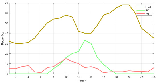
Figure 6.
Urban photovoltaic, wind power generation, and user load curves.
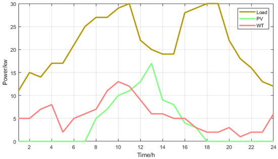
Figure 7.
Photovoltaic, wind power generation, and user load curves in agricultural and pastoral areas.
When the system is interconnected and operating, problems such as excessive or insufficient power output may occur in microgrids. For these two scenarios, the costs arising from the energy exchange between the microgrid and the utility grid must be fully considered. Therefore, when optimizing the scheduling of interconnected microgrid systems, it is necessary to consider not only the structure and operational characteristics of the microgrid system itself but also factors such as utility grid power and electricity prices.
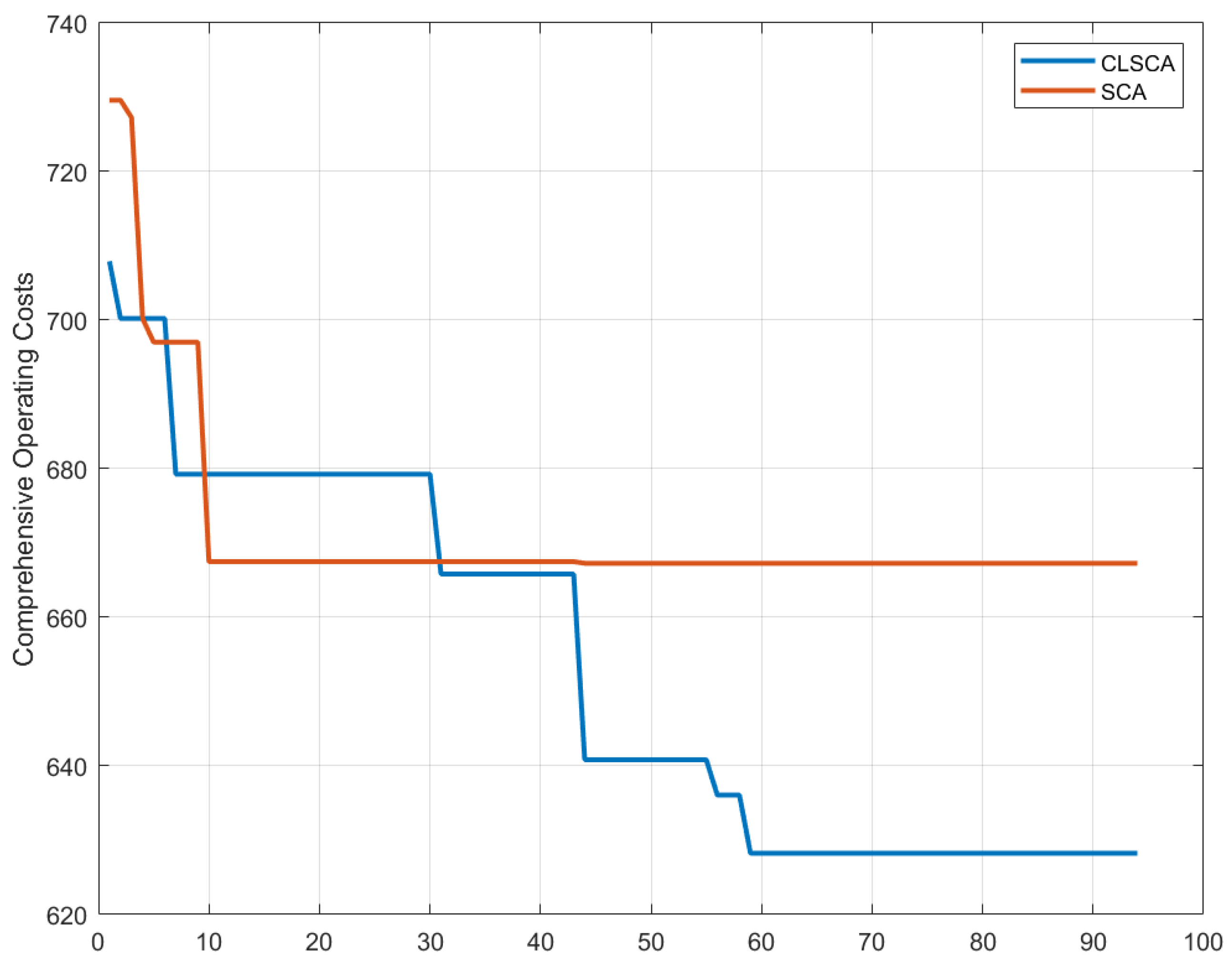
In this paper, an improved SCA (sine cosine algorithm) is employed to optimize the comprehensive cost of microgrids, taking into account the effects of electricity price fluctuations, environmental costs, and energy storage degradation costs. The improved optimal value evolution curves are shown in Figure 8 and Figure 9, where the vertical axis represents the optimal value of the comprehensive operating cost and the horizontal axis represents the number of iterations.
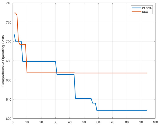
Figure 8.
Comprehensive cost convergence curve of urban microgrid.
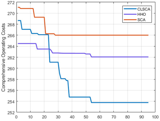
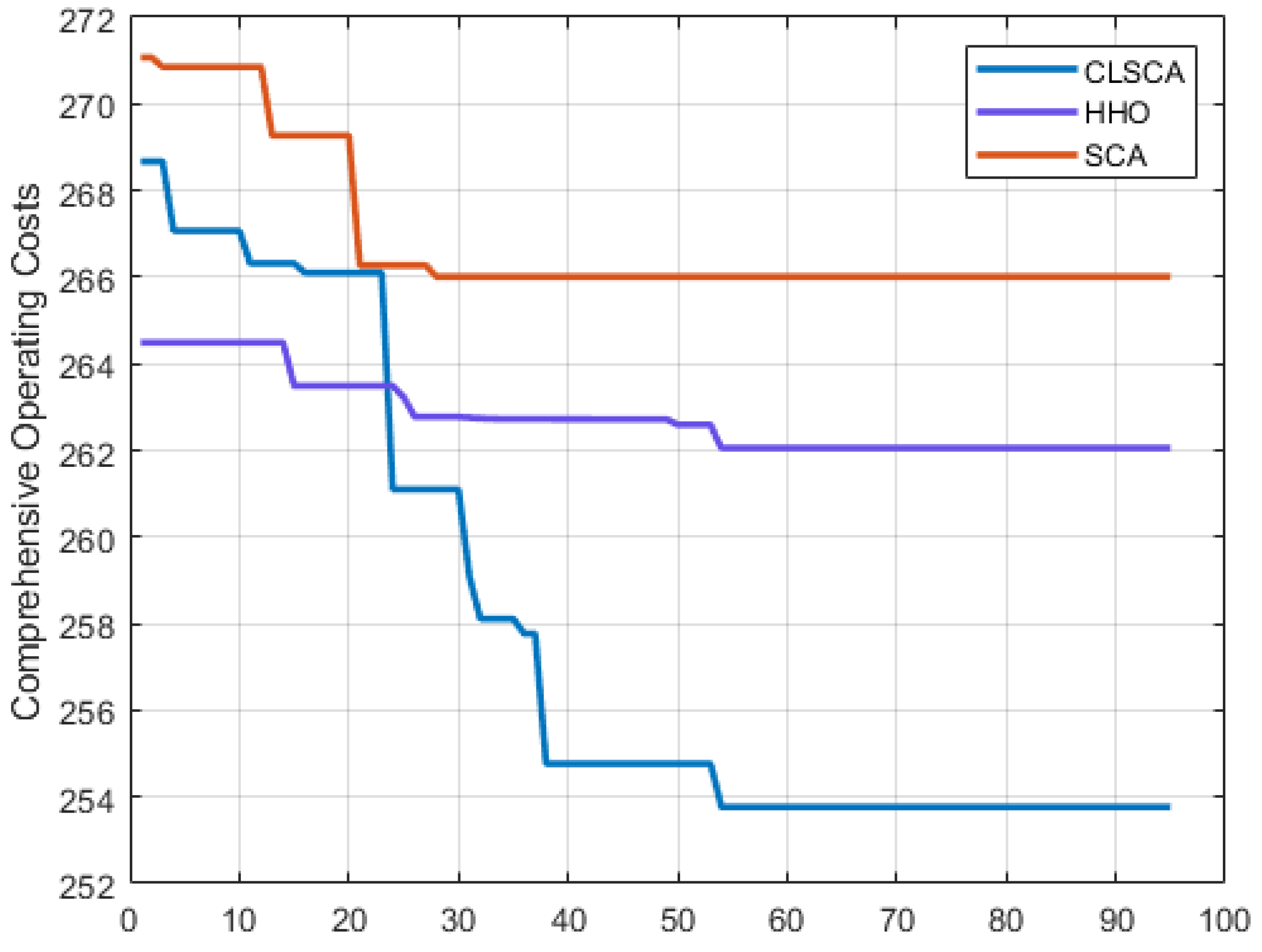
Figure 9.
Comprehensive cost convergence curve of microgrids in agricultural and pastoral areas.
Compared with the SCA and the HHO algorithm [31], the CLACS optimal value curve will not fall into the optimal solution so quickly, and its fitness is also reduced. The comprehensive costs of the SCA and HHO in the urban interconnection mode are 668.4 and 651.1, respectively, and the comprehensive cost of the CLSCA is 629.5. The comprehensive costs of the SCA and HHO in the independent agricultural and pastoral area mode are 266 and 262.1, respectively, and the comprehensive cost of CLSCA is 253.8. The algorithm before the improvement in the figure begins to converge in the early iteration, while the improved algorithm begins to converge after about 60 iterations. This shows that the improved algorithm has better global exploration capabilities.
Figure 10 depicts the output power of diesel generators, energy storage batteries, and the utility grid obtained using the CLSCA under the condition of minimizing comprehensive costs. It can be observed that during the early morning period with the lowest electricity prices, the utility grid increases its output power while the batteries charge themselves, thereby achieving energy scheduling during periods of low load and low electricity prices. Meanwhile, during the period of 11:00 to 16:00 when the output power of renewable energy generation is relatively high, the output power of all three components decreases. This period coincides with the peak wind and sunlight intensity throughout the day. Furthermore, at around 10:00 and 11:00, a portion of the microgrid’s generation is sold back to the utility grid when electricity prices are highest. By selling excess electricity to the utility grid during peak price periods, the microgrid effectively reduces costs.

Figure 10.
Urban output power.
After 18:00, as the output power of wind and solar generation reaches its lowest point of the day; both energy storage and the utility grid begin to increase their output power to compensate for the shortfall in renewable energy generation. As the clock approaches midnight, user loads enter a relatively low level, and the utility grid charges based on off-peak electricity prices. This lower electricity price prompts the batteries to start storing energy during the early morning hours. This flexible and dynamic adjustment significantly reduces the comprehensive operating costs of the microgrid.
Figure 11 shows the rated output power of the diesel generator and battery in the independent mode in the agricultural and pastoral areas. It can be seen that the battery is charged during the peak period of photovoltaic and wind power generation, and discharged during the low period of renewable energy power generation, which effectively adjusts the peak-to-valley difference of power load and ensures that the microgrid system can provide stable power services when the public network is offline.
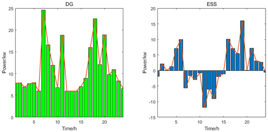
Figure 11.
Output power in agricultural and pastoral areas.
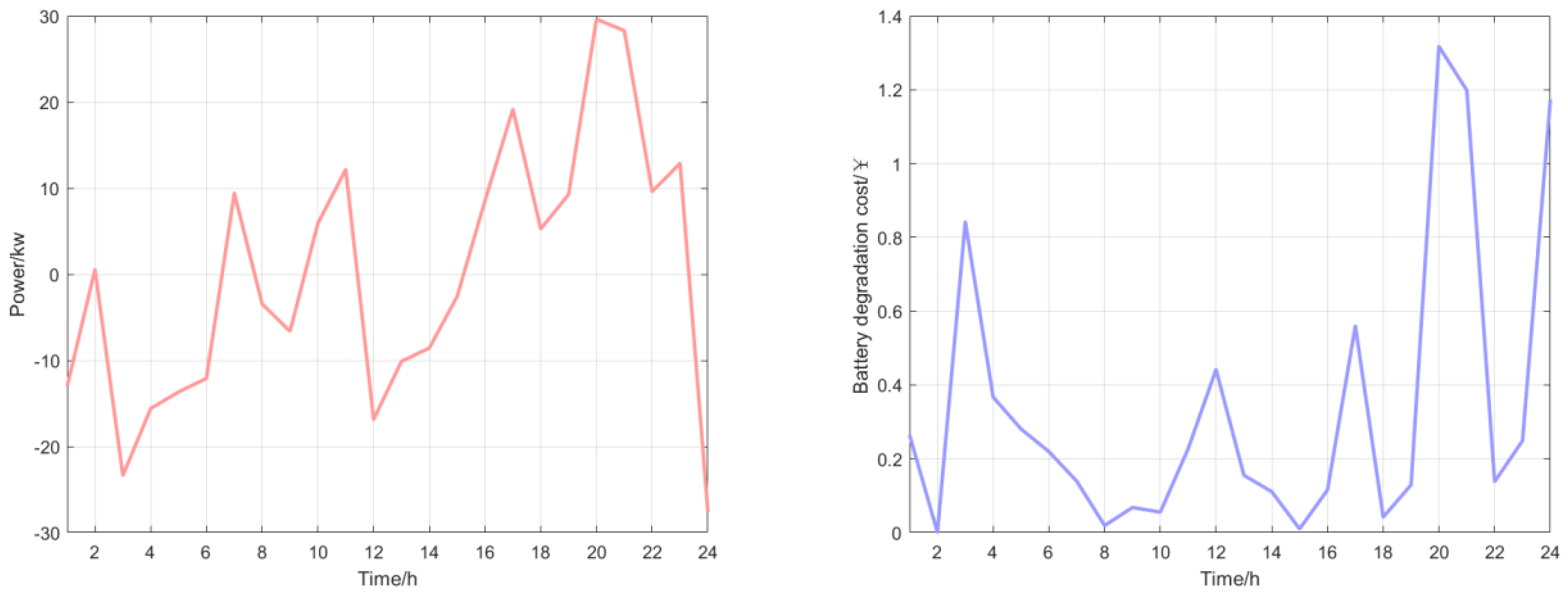
The following Figure 12 illustrates the output power and degradation cost of the battery. It can be observed that when the charging and discharging depths of the battery are relatively large, the degradation cost of the battery also increases accordingly. Therefore, adjusting the output power of energy storage reasonably can effectively reduce the degradation cost of the battery, thereby lowering the overall operating costs of the microgrid. The same applies to agricultural and pastoral areas.
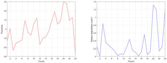
Figure 12.
Battery output power and degradation cost.
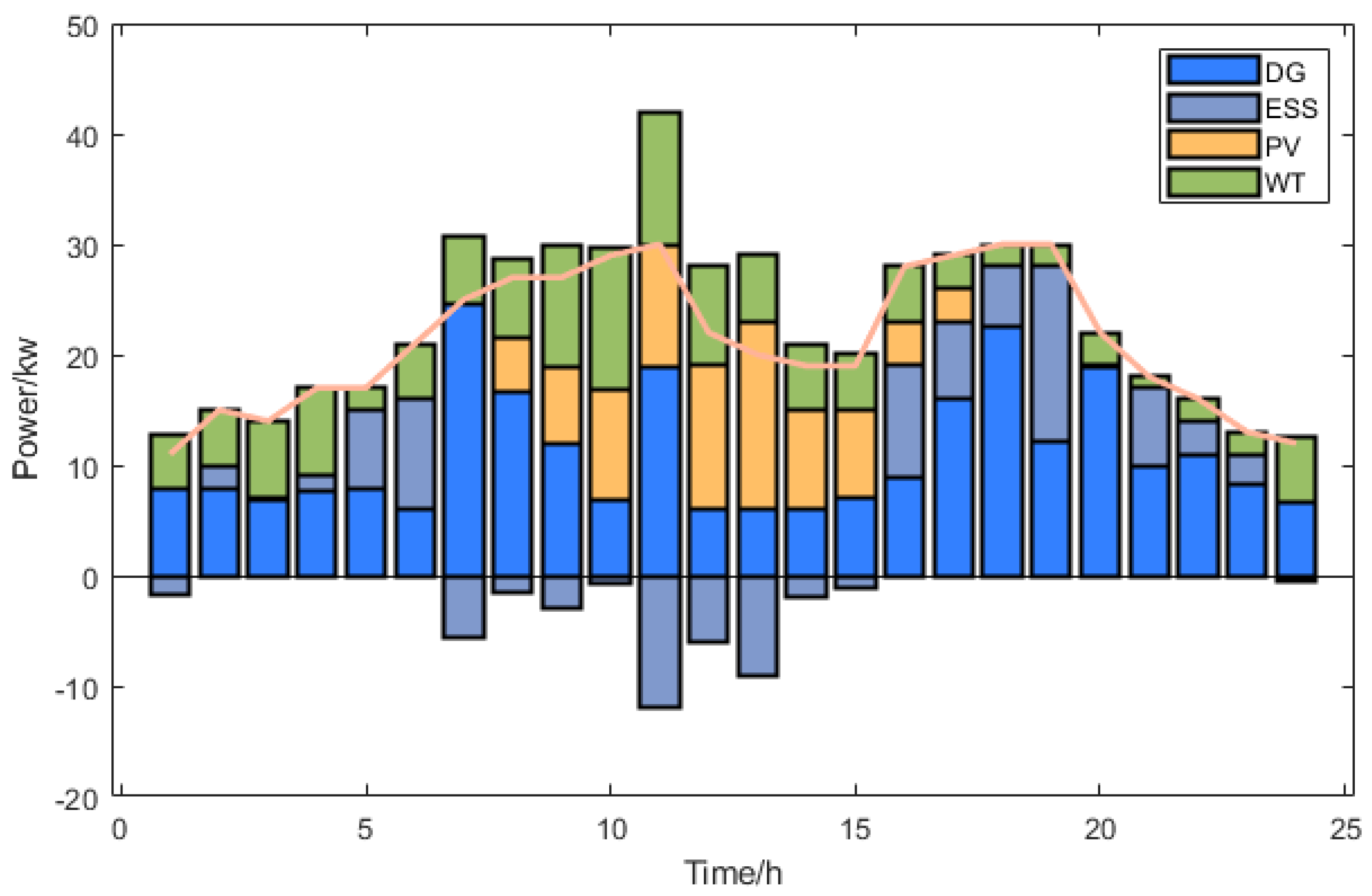
The predicted power balance diagrams obtained through the experiment are as follows, namely, Figure 13, the urban power balance diagram, and Figure 14, the agricultural and pastoral power balance diagram. The curves in the figure represent the changes in power load during the day. In the case of multiple limiting factors in renewable energy power generation, the output power of multiple power generation ends is adjusted in various ways to ensure the smooth operation of the load end of the microgrid system at a low operating cost.
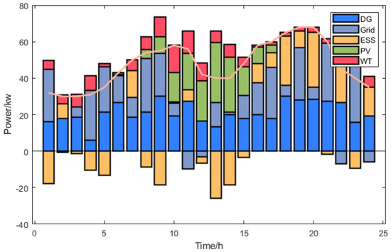
Figure 13.
Urban power balance diagram.
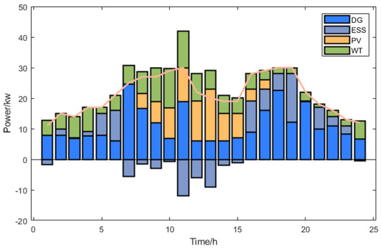
Figure 14.
Power balance diagram for agricultural and pastoral areas.
7. Conclusions
Microgrids, as flexible and organized electrical power systems, effectively integrates various generation sources and loads to meet regional electricity demands. The dynamic optimization of multiple distributed energy resources ensures the stability of the entire system, achieving efficient and reliable power supply. This paper analyzes the operational characteristics of distributed energy resources in microgrid systems, establishes mathematical models for wind power generation, photovoltaic generation, diesel generator generation, and battery energy storage, and clarifies their constraints. Based on this, a daily operational model for microgrids is constructed to reduce the overall operating costs of microgrid systems. Unlike previous studies that only consider economic costs and environmental management costs in microgrid operating costs, this paper incorporates battery degradation costs as an important influencing factor in comprehensive cost analysis of the system. The aim is to ensure the lowest operating costs of the microgrid while mitigating battery degradation through dynamic adjustments.
Energy management and cost planning in microgrids pose a complex nonlinear problem. Traditional methods are limited by dimensionality and data volume, making it challenging to solve such problems effectively. Therefore, this paper employs the SCA, a metaheuristic algorithm, to address this issue. The SCA offers advantages such as a simple structure and fast convergence. To achieve better optimization results, this study improves the SCA using two strategies: circle chaotic mapping and Levy flight. The effectiveness of the improved algorithm is validated through testing functions.
By applying the SCA and CLSCA to optimize the operating costs of the same microgrid system, this research provides a more comprehensive and accurate assessment of comprehensive costs. Finally, by comparing the application effects of the SCA and CLSCA, the superiority and reliability of the CLSCA in microgrid system optimization are verified. The results demonstrate that the model effectively reduces the comprehensive operating costs of microgrids, promoting their optimized operation.
Author Contributions
Methodology, Y.Z.; Validation, H.L.; Resources, B.C.; Writing—review & editing, C.W., D.D. and B.C. All authors have read and agreed to the published version of the manuscript.
Funding
This research received no external funding.
Data Availability Statement
The original contributions presented in this study are included in the article. Further inquiries can be directed to the corresponding author.
Conflicts of Interest
Author Yiming Zhao was employed by the company Inner Mongolia Electric Power (Group) Co., Ltd. Author Dong Du was employed by the company Inner Mongolia Electric Power Group Mengdian Information and Communication Industry Co., Ltd. The remaining authors declare that the research was conducted in the absence of any commercial or financial relationships that could be construed as a potential conflict of interest.
References
- Thirunavukkarasu, G.S.; Seyedmahmoudian, M.; Jamei, E.; Horan, B.; Mekhilef, S.; Stojcevski, A. Role of optimization techniques in microgrid energy management systems—A review. Energy Strategy Rev. 2022, 43, 100899. [Google Scholar] [CrossRef]
- Al-Shehri, M.A.; Guo, Y.; Lei, G. A Systematic Review of Reliability Studies of Grid-Connected Renewable Energy Microgrids. In Proceedings of the 2020 International Conference on Electrical, Communication, and Computer Engineering (ICECCE), Istanbul, Turkey, 12–13 June 2020; pp. 1–6. [Google Scholar] [CrossRef]
- Uddin, M.; Mo, H.; Dong, D.; Elsawah, S.; Zhu, J.; Guerrero, J.M. outstanding issues and future trends. Energy Strategy Rev. 2023, 49, 101127. [Google Scholar] [CrossRef]
- Qian, M.; Zhao, D.; Wu, F.; Zhu, L.; Chen, N.; Li, H.; Zhang, N. Review on modeling of wind power generation systems. In Proceedings of the 2019 IEEE Innovative Smart Grid Technologies—Asia (ISGT Asia), Chengdu, China, 21–24 May 2019; pp. 1958–1962. [Google Scholar] [CrossRef]
- Narang, A.; Farivar, G.G.; Tafti, H.D.; Pou, J. Power Reserve Control Methods for Grid-Connected Photovoltaic Power Plants: A Review. In Proceedings of the 2022 IEEE 7th Southern Power Electronics Conference (SPEC), Nadi, Fiji, 5–8 December 2022; pp. 1–5. [Google Scholar] [CrossRef]
- Duan, Y.; Zhao, Y.; Hu, J. An initialization-free distributed algorithm for dynamic economic dispatch problems in microgrid: Modeling, optimization and analysis. Sustain. Energy Grids Netw. 2023, 34, 101004. [Google Scholar] [CrossRef]
- Dey, B.; Misra, S.; Pedro, F.; Marquez, G. Microgrid system energy management with demand response program for clean and economical operation. Appl. Energy 2023, 334, 120717. [Google Scholar] [CrossRef]
- Zhao, Z.; Xu, J.; Guo, J.; Ni, Q.; Chen, B.; Lai, L.L. Robust Energy Management for Multi-Microgrids Based on Distributed Dynamic Tube Model Predictive Control. IEEE Trans. Smart Grid 2024, 15, 203–217. [Google Scholar] [CrossRef]
- Wongdet, P.; Boonraksa, T.; Boonraksa, P.; Pinthurat, W.; Marungsri, B.; Hredzak, B. Optimal Capacity and Cost Analysis of Battery Energy Storage System in Standalone Microgrid Considering Battery Lifetime. Batteries 2023, 9, 76. [Google Scholar] [CrossRef]
- Hemmati, M.; Bayati, N.; Ebel, T. Integrated Optimal Energy Management of Multi-Microgrid Network Considering Energy Performance Index: Global Chance-Constrained Programming Framework. Energies 2024, 17, 4367. [Google Scholar] [CrossRef]
- Vásquez, L.O.P.; Ramírez, V.M.; Thanapalan, K. A Comparison of Energy Management System for a DC Microgrid. Appl. Sci. 2020, 10, 1071. [Google Scholar] [CrossRef]
- Kharrich, M.; Kamel, S.; Abdel-Akher, M.; Eid, A.; Zawbaa, H.M.; Kim, J. Optimization based on movable damped wave algorithm for design of photovoltaic/wind/diesel/biomass/battery hybrid energy systems. Energy Rep. 2022, 8, 11478–11491. [Google Scholar] [CrossRef]
- Dayalan, S.; Rathinam, R. Energy management of a microgrid using demand response strategy including renewable uncertainties. Int. J. Emerg. Electr. Power Syst. 2021, 22, 85–100. [Google Scholar] [CrossRef]
- Dong, H.; Fu, Y.; Jia, Q.; Zhang, T.; Meng, D. Low carbon optimization of integrated energy microgrid based on life cycle analysis method and multi time scale energy storage. Renew. Energy 2023, 206, 60–71. [Google Scholar] [CrossRef]
- Wang, K.; Xue, Y.; Shahidelhpour, M.; Chang, X.; Li, Z.; Zhou, Y. Resilience-Oriented Two-Stage Restoration Considering Coordinated Maintenance and Reconfiguration in Integrated Power Distribution and Heating Systems. IEEE Trans. Sustain. Energy 2025, 16, 124–137. [Google Scholar] [CrossRef]
- Li, Z.; Wu, L.; Xu, Y.; Zheng, X. Stochastic-Weighted Robust Optimization Based Bilayer Operation of a Multi-Energy Building Microgrid Considering Practical Thermal Loads and Battery Degradation. IEEE Trans. Sustain. Energy 2022, 13, 668–682. [Google Scholar] [CrossRef]
- Ahshan, R.; Nasiri, N.; Al-Badi, A.H.; Hosseinzadeh, N. Control and Dynamic Analysis of an Isolated Microgrid System: A Case Study. In Proceedings of the 2020 6th IEEE International Energy Conference (ENERGYCon), Gammarth, Tunisia, 28 September–1 October 2020; pp. 254–259. [Google Scholar] [CrossRef]
- Yin, M.; Li, L.; Yan, H.; Ren, M.; Wang, J.; Ma, M. Application scenario analysis of microgrid based on typical structure classification of microgrid. In Proceedings of the 2023 IEEE 6th International Electrical and Energy Conference (CIEEC), Hefei, China, 12–14 May 2023; pp. 2711–2716. [Google Scholar] [CrossRef]
- Popov, N.S.; Anibroev, V.I.; Mosin, M.M. Study of processes that cause degradation of lithium-ion batteries. In Proceedings of the 2021 3rd International Youth Conference on Radio Electronics, Electrical and Power Engineering (REEPE), Moscow, Russia, 11–13 March 2021; pp. 1–4. [Google Scholar] [CrossRef]
- Mocera, F.; Somà, A.; Clerici, D. Study of aging mechanisms in lithium-ion batteries for working vehicle applications. In Proceedings of the 2020 Fifteenth International Conference on Ecological Vehicles and Renewable Energies (EVER), Monte-Carlo, Monaco, 10–12 September 2020; pp. 1–8. [Google Scholar] [CrossRef]
- Yarimca, G.; Cetkin, E. Review of Cell Level Battery (Calendar and Cycling) Aging Models: Electric Vehicles. Batteries 2024, 10, 374. [Google Scholar] [CrossRef]
- Martins, M.A.I.; Rhode, L.B.; Almeida, A.B.D. A Novel Battery Wear Model for Energy Management in Microgrids. IEEE Access 2022, 10, 30405–30413. [Google Scholar] [CrossRef]
- Wang, L. Merchant Energy Storage Investment Analysis Considering Multi-Energy Integration. Energies 2023, 16, 4695. [Google Scholar] [CrossRef]
- Park, J.; Choi, J.; Jo, H.; Kodaira, D.; Han, S.; Acquah, M.A. Life Evaluation of Battery Energy System for Frequency Regulation Using Wear Density Function. Energies 2022, 15, 8071. [Google Scholar] [CrossRef]
- Ji, Y.; Hou, X.; Pang, C.; Liu, J.; Lv, Z. Bi-Level Method of Islanded Microgrid Optimal Sizing Based on Life Cycle Cost. In Proceedings of the 2019 IEEE 3rd International Electrical and Energy Conference (CIEEC), Beijing, China, 7–9 September 2019; pp. 1366–1371. [Google Scholar] [CrossRef]
- Chen, T.; Bu, S.; Liu, X.; Kang, J.; Yu, F.R.; Han, Z. Peer-to-Peer Energy Trading and Energy Conversion in Interconnected Multi-Energy Microgrids Using Multi-Agent Deep Reinforcement Learning. IEEE Trans. Smart Grid 2022, 13, 715–727. [Google Scholar] [CrossRef]
- Abualigah, L.; Diabat, A. Advances in Sine Cosine Algorithm: A comprehensive survey. Artif. Intell. Rev. 2021, 54, 2567–2608. [Google Scholar] [CrossRef]
- Altay, V.; Alatas, B. Bird swarm algorithms with chaotic mapping. Artif. Intell. Rev. 2020, 53, 1373–1414. [Google Scholar] [CrossRef]
- Jiang, A.; Gao, Y. A Gaussian convolutional optimization algorithm with tent chaotic mapping. Sci. Rep. 2024, 14, 31027. [Google Scholar]
- Gupta, R.; Pal, R. Biogeography-Based Optimization with LéVY-Flight Exploration for Combinatorial Optimization. In Proceedings of the 2018 8th International Conference on Cloud Computing, Data Science & Engineering (Confluence), Noida, India, 11–12 January 2018; pp. 664–669. [Google Scholar] [CrossRef]
- Peng, L.; Cai, Z.; Heidari, A.A.; Zhang, L.; Chen, H. Hierarchical Harris hawks optimizer for feature selection. J. Adv. Res. 2023, 53, 261–278. [Google Scholar] [CrossRef]


Disclaimer/Publisher’s Note: The statements, opinions and data contained in all publications are solely those of the individual author(s) and contributor(s) and not of MDPI and/or the editor(s). MDPI and/or the editor(s) disclaim responsibility for any injury to people or property resulting from any ideas, methods, instructions or products referred to in the content. |
© 2025 by the authors. Licensee MDPI, Basel, Switzerland. This article is an open access article distributed under the terms and conditions of the Creative Commons Attribution (CC BY) license (https://creativecommons.org/licenses/by/4.0/).