Abstract
To ensure a reliable and safe operation of battery systems in various applications, the system’s internal states must be observed with high accuracy. Hereby, the Kalman filter is a frequently used and well-known tool to estimate the states and model parameters of a lithium-ion cell. A strong requirement is the selection of a suitable model and a reasonable initialization, otherwise the algorithm’s estimation might be insufficient. Especially the process noise parametrization poses a difficult task, since it is an abstract parameter and often optimized by an arbitrary trial-and-error principle. In this work, a traceable procedure based on the genetic algorithm is introduced to determine the process noise offline considering the estimation error and filter consistency. Hereby, the parameters found are independent of the researcher’s experience. Results are validated with a simulative and experimental study, using an NCA/graphite lithium-ion cell. After the transient phase, the estimation error of the state-of-charge is lower than 0.6% and for internal resistance smaller than 4mΩ while the corresponding estimated covariances fit the error well.
1. Introduction
In today’s management systems of lithium-ion batteries, state estimation is a crucial part. In the context of battery electric vehicles, the precise estimation of the state-of-charge (SOC) enables reliable range prediction, whereas estimation of the battery’s resistance is essential to determine the currently available power. Besides other approaches, the Kalman filter (KF) is widely used as a model based state and parameter estimator for this task [1]. It comprises on the one hand a prediction step based on the battery current and a battery model, and on the other hand a correction step, which uses the terminal voltage of the battery. It is worth noting that KFs are optimal estimators with respect to the squared estimation error under certain assumptions. These involve that the process noise and measurement noise are Gaussian distributed, zero mean and not correlated with each other. Furthermore, the covariances of the process and measurement noise have to be known. While the voltage measurement noise is easily determinable, selecting an optimal process noise covariance matrix is a challenging task and still an unsolved problem. This is commonly known as Kalman filter tuning.
Former approaches of filter tuning such as bayesian estimation [2,3], maximum likelihood estimation [4], correlation methods [5,6] or covariance matching [7,8] reach back to the 1970s and are intensively discussed in the literature [2,9,10]. However, besides the heavy computational costs of the two former approaches, a common drawback of the correlation method is the limitation to stable systems, unlike random-walk models used in this work. Furthermore, according to [11] the covariance matching leads to systematic errors. Hence, nowadays filter tuning is still too often realized by trial-and-error of an experienced engineer or researcher.
KF tuning can be seen as an optimization problem, whereas a process noise covariance is sought under certain optimization objectives. Most commonly, only the estimation error of a few states [3,12,13] or the measurement error [14,15] is minimized. Within this work, we present a multi-objective optimization approach that (a) minimizes the estimation errors of all estimated states and parameters and (b) maximizes the consistency of the estimation results. The latter is a new approach to the author’s best knowledge. Considering magnitude and consistency of the estimation error leads to reasonable results and avoids overfitting to training data.
The large optimization space of the process noise covariance is challenging and requires an efficient search algorithm. Furthermore, the relation between the process noise covariance and the estimation result is highly non-linear and hard to predict. Therefore, we chose the genetic algorithm for this optimization problem. Genetic algorithms (GAs) are heuristic methods and are based on the work of John Holland and his colleagues. Since they are gradient free and start with a population of several initial points, they efficiently search solutions in large spaces despite little prior knowledge and are suitable for a wide range of problems [16,17]. By using an optimization approach for tuning the Kalman filter, the results are traceable, objective and independent of the researcher’s experience. In ref. [13], the authors use a GA for filter tuning within a battery management system. However, the parameters of the optimization algorithm are not selected consciously and only the mean absolute errors of SOC and ohmic resistance are taken as optimization objectives.
In this paper, the process noise covariance of an extended Kalman filter (EKF) is optimized, in order to estimate the states and parameters of a lithium-ion cell’s equivalent circuit model (ECM). In contrast to the existing literature, we use three optimization objectives in combination with a GA to find the best set of solutions with respect to both, estimation accuracy and consistency. The remainder of this contribution is organized as follows: Section 2 explains the used model and the joint extended Kalman filter. In Section 3 the optimization methodology including the GA, objective selection and initialization process is described. At the end of this work, simulative and experimental results are demonstrated, compared and discussed.
2. State and Parameter Estimation
2.1. Battery Model
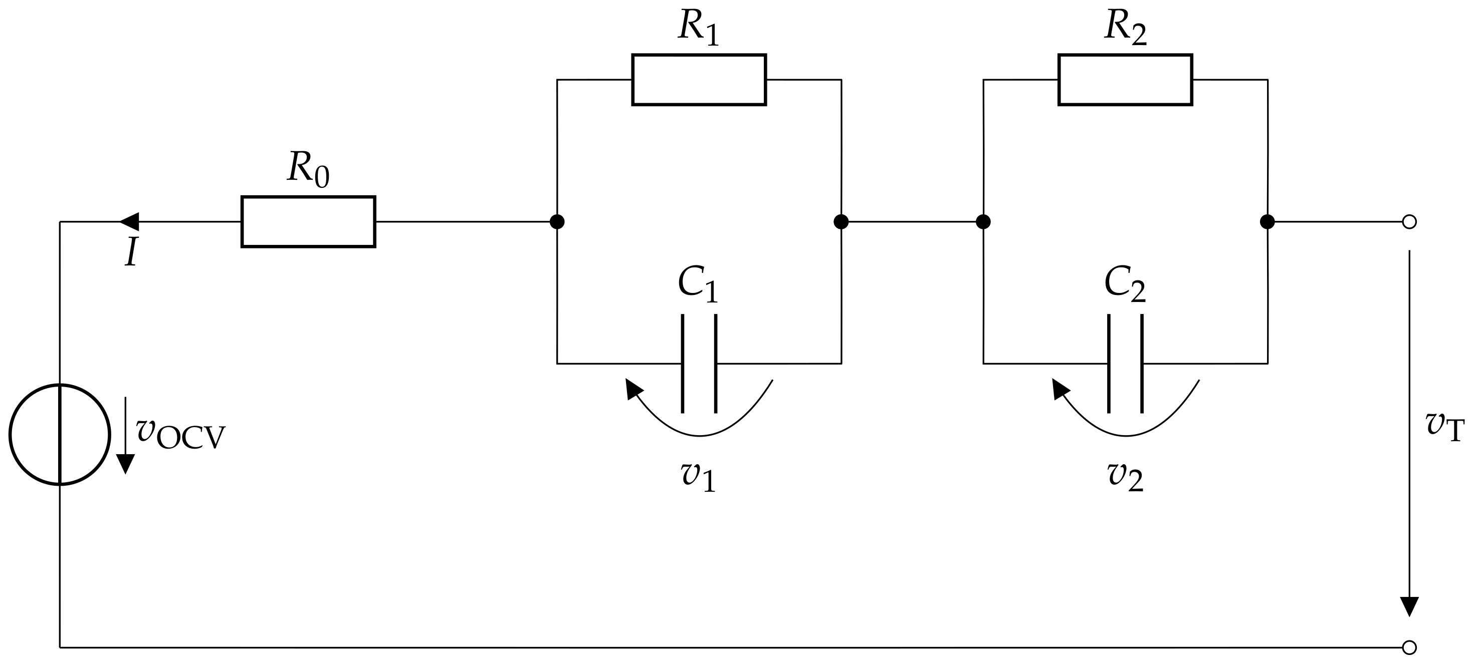
The ECM, shown in Figure 1, is used to model the lithium-ion battery’s electrical behavior. It consists of an SOC-dependent voltage source , to represent the ohmic resistant and two RC elements (, and , , respectively). Some authors in the literature [18,19,20] link the first RC element to the charge transfer resistance and the double layer capacitance and the second RC element to the diffusion resistance and capacitance. However, more generally, the voltage response of lithium-ion cells can be described by an arbitrary number of RC elements. Adding more RC elements can improve the model accuracy but also leads to higher computational costs. Refs. [21,22] found two RC elements to be a reasonable trade-off. All parameters depend on SOC, temperature and the aging state of the battery. In our case only the SOC dependence is considered since the temperature is assumed to be constant during all experiments, and aging is neglected for simplicity. In addition, the data used is recorded over a short period of time. Therefore, it is assumed that aging has no influence on the operation of the battery. The load current I and the terminal voltage are measured during operation. The following is based on [23,24]. Using the mesh rule and the ECM in Figure 1 leads to the measurable terminal voltage of the battery:
The differential equations of the two RC elements are given as
with and the SOC is obtained by integrating the current over time:
Hereby, is the initial state-of-charge and the available capacity of the cell. The coulombic efficiency of lithium-ion batteries is high and therefore set to . According to (3) a positive current I is defined to charge the lithium-ion cell.

Figure 1.
ECM of the battery with two RC elements.
These equations form a discrete SISO (single input single output) state space model as follows:
where is the system matrix, the input matrix, the output matrix, D the feed through value, u the input, y the output and the state vector. By defining the state vector to the state space model results with , as step size, and in
Please note that the first element of the output matrix has to be updated in every time step based on the current SOC. For simplicity, the two time constants of the RC elements are kept constant. This leads in total to three states (SOC, , ) and three parameters (, , ), respectively.
2.2. Kalman Filter
The KF [25] is based on the state space model, whereby a zero mean and Gaussian distributed process noise with and measurement noise is added. The states and the parameters of the model are estimated simultaneously by augmenting the parameter vector to the state vector. Please note, for a simple notation all states and parameters are combined in the state vector with . Since there is no prior knowledge about the parameters’ change over time, a random-walk model is used. Therefore the equation of the state-space model for the joint estimation can be formulated as follows [24]:
Since the system has a non-linear behavior, the discrete state-space system is shown in (10) and (11) with the non-linear system equation and output equation h.
To solve the non-linear state-space system, an EKF is applied, which calculates the system matrix and the output matrix by linearizing the system at each time step with the Jacobean matrix. Algorithm 1 shows the whole procedure of the EKF.
| Algorithm 1 Extended Kalman filter |
| Initialization: |
| Prediction: |
| Update: |
According to Yang et al. [26] the estimation is stabilized by neglecting all covariances between states, which are not linked in reality. Therefore, all irrelevant covariances are set to zero after each iteration of the filter algorithm as shown by Schneider et al. [24]:
The linked states are only the polarization voltages with their corresponding resistances of the RC elements.
3. Optimization Methodology
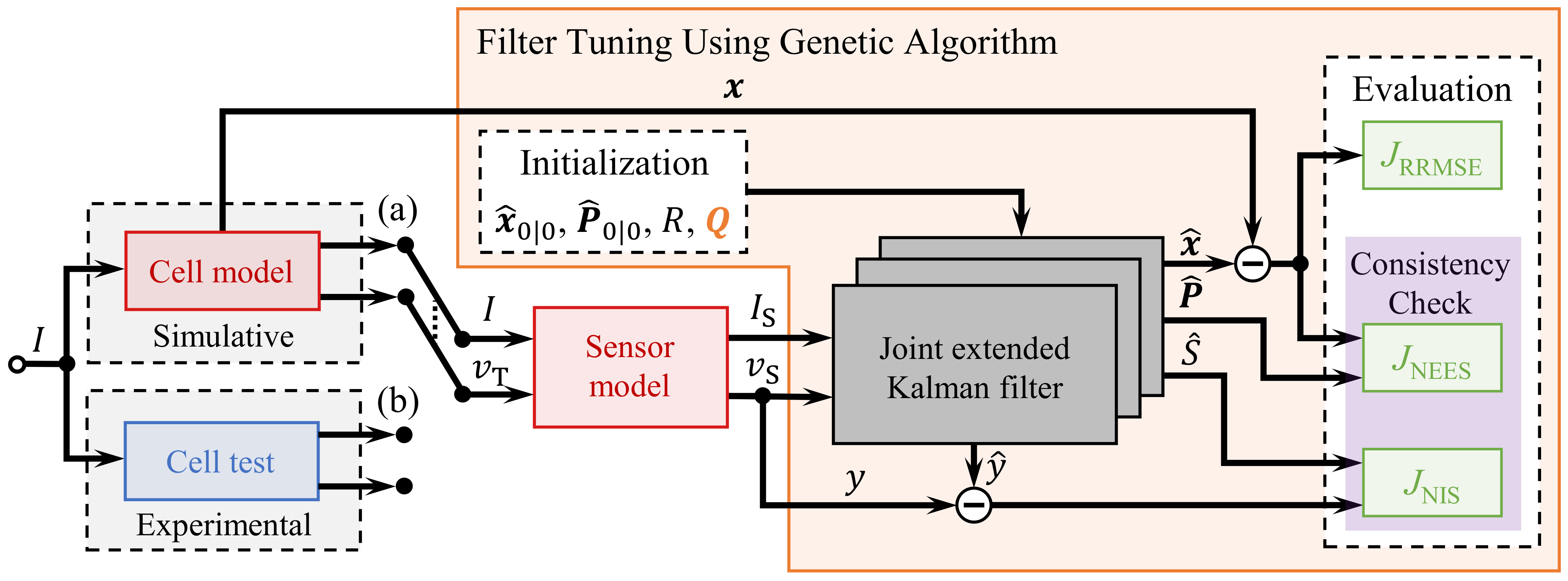
The proposed methodology to optimize the process noise is shown in Figure 2. For filter tuning, the input load current I is predefined by the WLTP (Worldwide Harmonized Light-Duty Vehicles Test Procedure) driving profile shown in Figure 3a. Subsequently, the validation is performed using the UDDS (Urban Dynamometer Driving Schedule) profile in Figure 3b. Both provide a realistic current profile with discharge, charge and rest phases. The terminal voltage is obtained either by simulation or by measurements in case of experiments. Afterwards, a sensor model is used to add a known normal distributed noise before the data is used to estimate states and parameters with the EKF. Those estimation outputs are compared with the reference states and parameters to calculate the estimation error. Please note that in case of experiments, the reference states and parameters are also obtained from simulations, since the states and parameters are not accessible in reality. To optimize the process noise , the estimation error and two consistency values defined in Section 3.2 are evaluated. Therefore a multi-objective optimization method is used. The GA is suitable for this specific task.
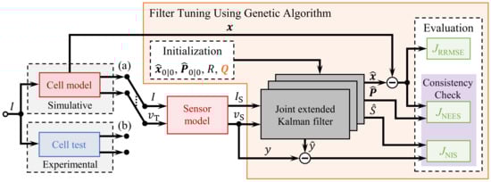
Figure 2.
Optimization methodology for (a) the simulative and (b) the experimental case based on GAs.
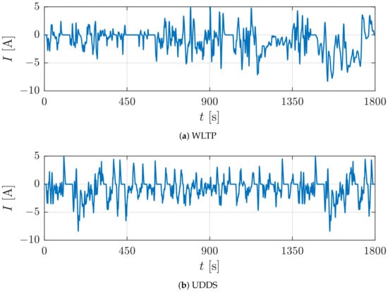
Figure 3.
Current profiles for (a) the filter tuning process with the WLTP cycle and (b) validation with the UDDS cycle.
3.1. Genetic Algorithm
GAs are based on the “survival of the fittest” principle [17]. They start with an initial population with a certain amount of possible solutions for the problem, called individuals. In our case each individual contains the six diagonal elements of , which can be inherited to the next generation. For each individual, a fitness values is calculated representing the suitability of the solution for the problem at hand. Furthermore, the probability of an individual to be selected to inherit its properties or to be passed on to the new generation increases with a better fitness. A new generation is built by elite individuals (duplication), recombination and mutation [15]. This whole process repeats itself leading to an extinction of bad individuals and properties until defined end criteria are met. As already pointed out, a multi-objective optimization is needed. Therefore the result is not a single solution, but a set of solutions forming a Pareto front [27]. Here, no objective can be improved without worsening at least another one.
3.2. Object Selection
For the multi-objective optimization several objectives need to be defined. For the KF estimation, it is essential to obtain an accurate and consistent filter. To determine the accuracy, the relative root mean squared error (RRMSE) is calculated separately for all entries of the state vector over K time steps according to (13), where the root mean squared error (RMSE) in the numerator is divided by the mean absolute value of the observations.
The normalization ensures a unitless error measure. Furthermore, features with larger value ranges do not have a greater influence on the following mean value calculation. The RRMSE is averaged over all entries of the state vector and over the number of Monte-Carlo runs N as follows
to obtain one single accuracy measure for the estimator. According to [28], a KF is consistent if the estimation error and the innovation e have an expectation of zero and the covariance or , respectively. Those conditions can be tested by evaluating the distribution of the normalized estimation error square (NEES) and normalized innovation squared (NIS) over several Monte-Carlo runs with:
and
where is a chi-square-distribution with the degree of freedom . In order to use consistency as an optimization objective, a quantification method is required. This is implemented following Oshman et al [16]. The probabilities and for each time step are calculated as follows
and sorted in ascending order of magnitude. For a consistent KF, the probabilities must lie on the angle bisector over the normalized index. By calculating the area between the resulting curve and the angle bisector a consistency value can be obtained
where and are limited between 0 and 0.5. Smaller values are indicates to a more consistent KF.
3.3. Setup and Model Characterization
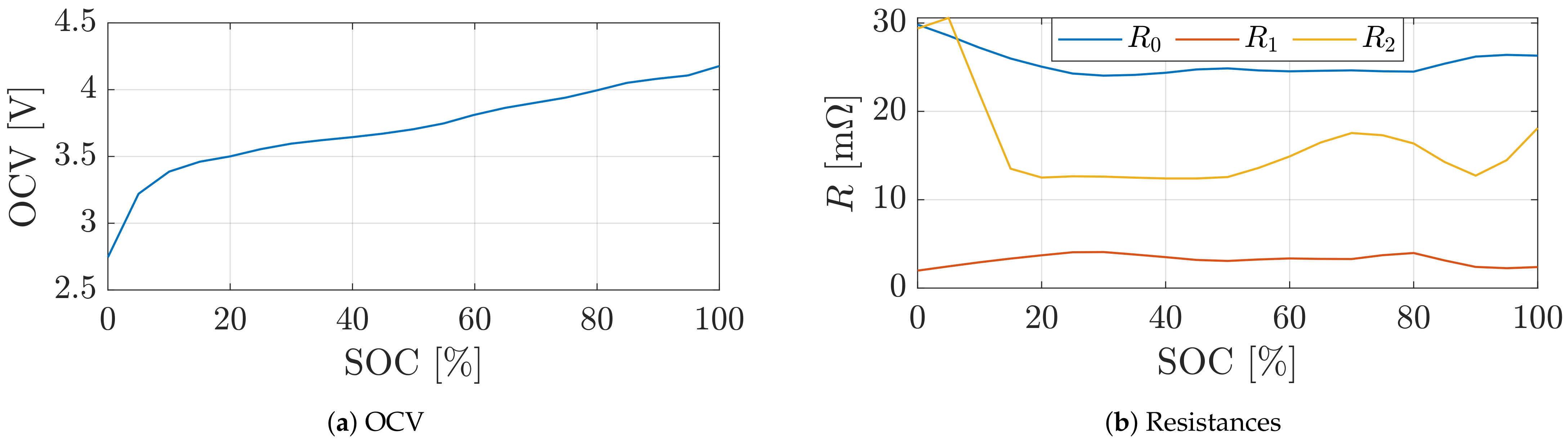
To determine the model parameters for simulations and to validate the proposed method with experiments, an experimental setup and a characterization procedure is required. The used lithium-ion battery cells INR18650-25R from Samsung have NCA (lithium nickel cobalt aluminum oxide) as cathode and graphite as anode. The specifications of this cell type according to the data sheet are shown in Table 1. All experiments are conducted with the LBT21084 Arbin battery test system (60 A/5 V) within a Binder temperature chamber (KB 115). The temperature is set to 25 °C. After a 1C discharge capacity test, the open circuit voltage (OCV) of the used cell is measured in the charge and discharge direction over the whole SOC range with a step size of 2%. By averaging and interpolating the measured OCV in the charge and discharge direction for one SOC step, the OCV function shown in Figure 4a is obtained. Due to averaging possible hysteresis effects are neglected. The parameters , and in Figure 4b are obtained by a current pulse test with 2C and a duration of 1 s and 20 s from to SOC in steps. The searched parameters are optimized by minimizing the RMSE between modeled and measured terminal voltage with the help of the MATLAB function fminsearch. Hereby s and s applies. For more information about the characterization, we refer to [24].

Table 1.
Lithium-ion cell specification.
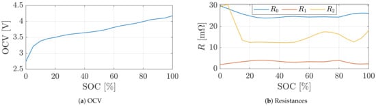
Figure 4.
Cell characterization results for the (a) OCV and (b) the resistances of the ECM over the entire SOC range.
3.4. Implementation
To show the benefits and the feasibility of the proposed optimization methodology, simulations are conducted. The initial SOC is approximately for all studies. The sensor noise is modeled as a zero mean Gaussian distribution with a current standard deviation of mA and a voltage standard deviation of . This leads to the variance of the measurement noise
The step size in the simulative as well as in the experimental study is 0.1 s. To ensure statistical reasonable results the KF is evaluated over Monte-Carlos runs. In each Monte-Carlo run the state vector is reinitialized, such that (24) applies [28].
The covariance is initialized as in (25) such that the standard deviation is in the order of of the true initial entries of . Since the initial values of the polarization voltages are zero, the standard deviation is set to mV and mV, respectively.
The process noise is optimized using the multi-objective GA using the built-in function gamultiobj from MATLAB 2021b. The most important GA options are shown in Table 2. Hereby, only the logarithm of the six diagonal elements of the matrix are optimized while all other entries are set to zero. The upper and lower limit of the decision variable space are set based on the authors’ experience to reduce the set of possible solutions for a faster convergence of the algorithm. The objectives shown in the previous chapter are combined in the fitness function . The number of individuals forming the Pareto front can be set as a ratio of the population size via the Pareto fraction (here: ). The only selection function available for gamultiobj is the tournament selection, where a certain number of individuals compete against each other, and only the best one is selected [29,30]. The crossover function crossoverintermediate determines how new individuals are generated by recombination. Two parents span an dimensional space in which the resulting child is randomly located [31]. The ratio of crossover children in the new generation is specified by the crossover fraction. While crossover is based on existing individuals and searches around their properties, mutation is required to introduce new properties to the individuals and therefore prevent early convergence of the algorithm [30]. The mutation function mutationadaptfeasible determines the direction of mutation adaptively depending on the previous generation and its fitness [31].
Table 2.
GA optimization options.
4. Results and Discussion
For evaluation of the estimation results, the RMSE in (26) is calculated for each state and parameter beside the already explained optimization objectives. The RMSE is additionally averaged over 30 Monte-Carlo runs. Please note, that for simulative and experimental studies the reference values are obtained from simulation and model characterization. In real experiments, it is not possible to obtain the non-measurable states and parameters directly.
In order to be able to assess the error measures, the range of values occurring in our investigations for each state and parameter is given in Table 3. The cell is discharged with the WLTP and UDDS profile from 90% SOC to 69% and 75%, respectively.
Table 3.
Occurring minimal and maximal values for each state and parameter within our investigation.
4.1. Simulative Study
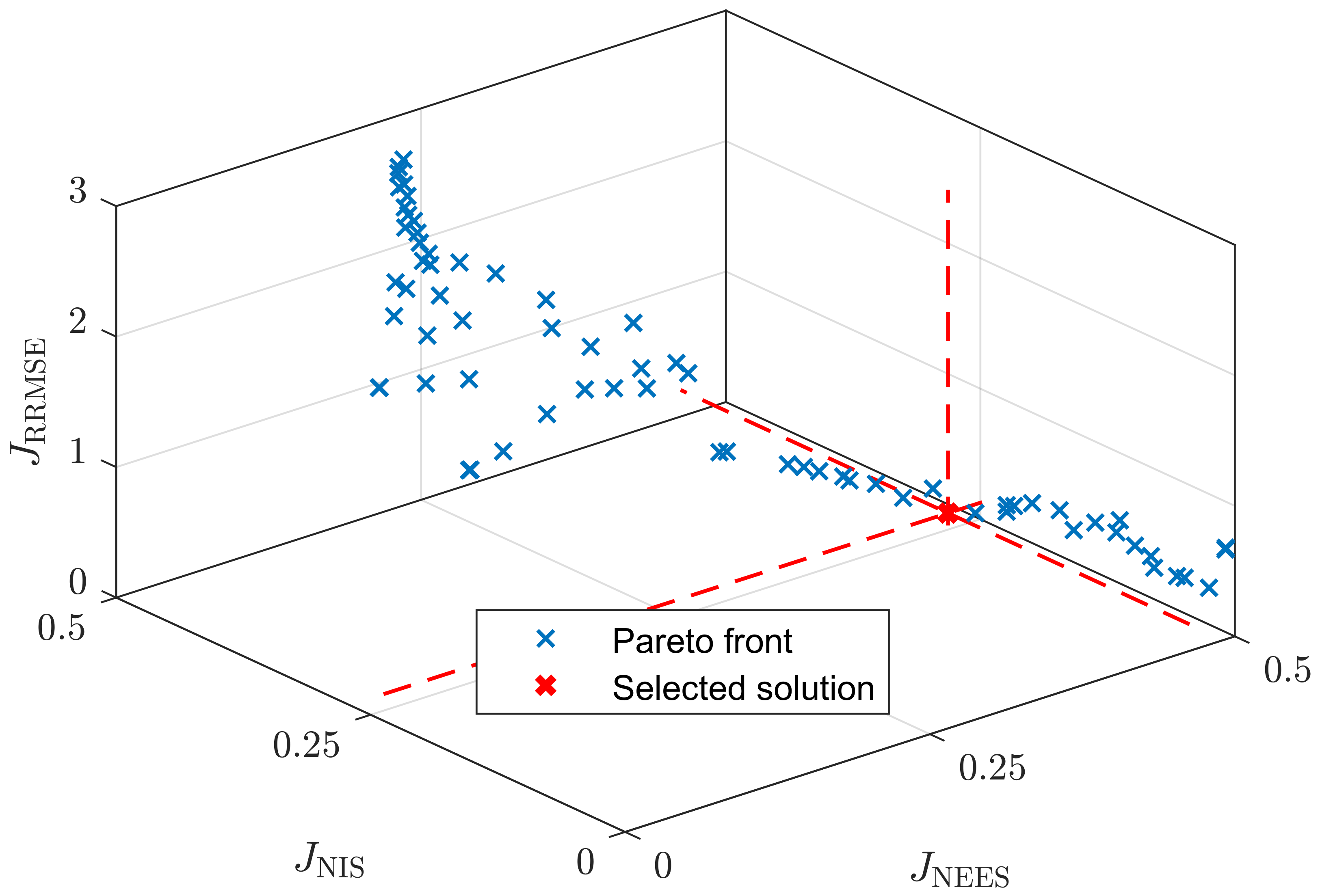
In the simulative case, the optimization process using the WLTP cycle converges after around 57 generations resulting in the blue Pareto front shown in Figure 5. The trade-off between all three optimization objectives becomes obvious. As soon as one of the consistency values ( or ) is minimized, both the other one as well as the estimation error become large. The controversial behavior is also observable in Figure 6, where the entries of process noise matrix are plotted decadic logarithmized over the individual consistency optimization objectives. For example, in Figure 6a rises for higher and values while in Figure 6b decreases. Please note, that and are the variances of the SOC and , respectively. The trend lines displayed with different colors indicate that the parameters are not changing arbitrarily. Regardless of two outliers in Figure 6b, the sensitivity of the entries to the consistency measures is limited. A small change in the parameterization usually leads to only a small change in consistency. Furthermore, while it is possible to reach values smaller than 0.02, it is harder to minimize with values always greater than 0.13. In our case, we choose the individual with the smallest euclidean distance to the origin of the coordinate system in the objective space with , and corresponding to the red dashed lines in Figure 5 and Figure 6. The resulting process noise is
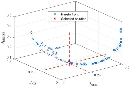
Figure 5.
Pareto front (blue) and the selected solution (red) in the objective space for the simulative case.
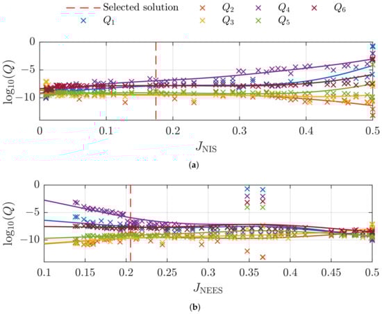
Figure 6.
Dependence of the (a) and (b) values on the logarithm of the process noise.
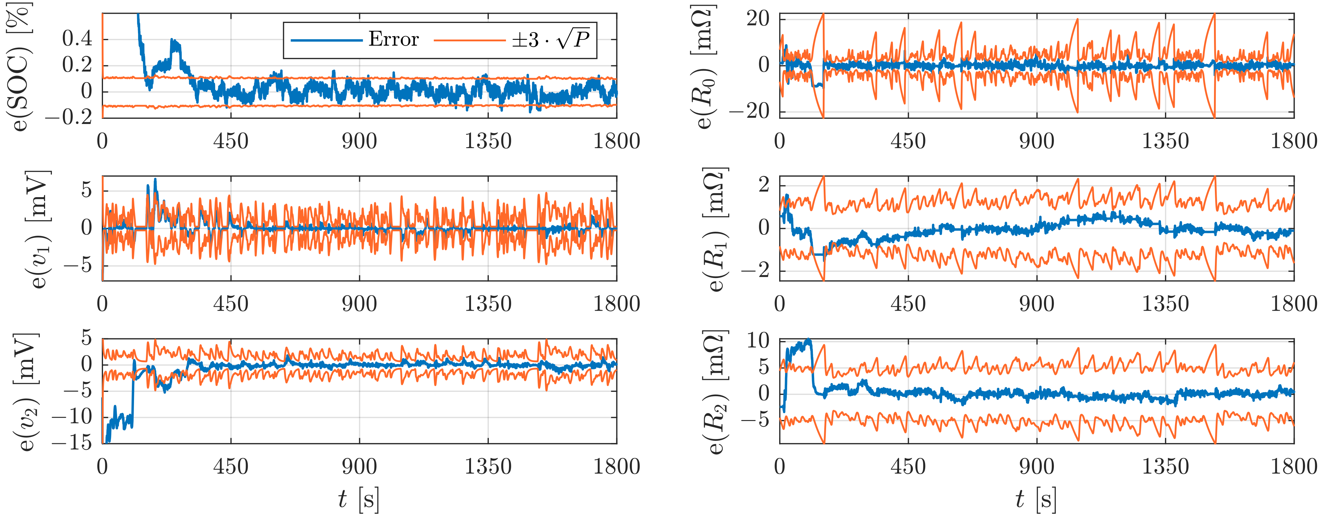
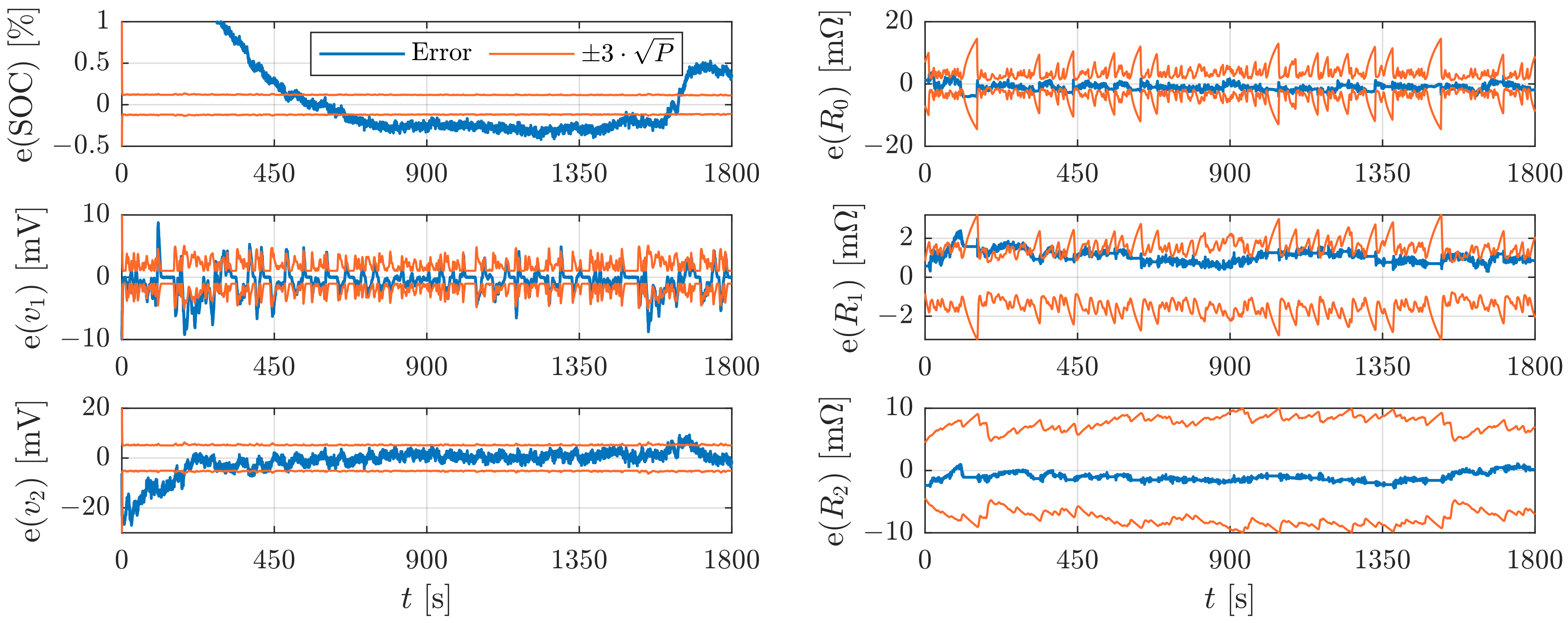
For validation the optimized process noise is used to estimate the states and parameters for the UDDS cycle. Figure 7 shows in blue the error of all states and parameter and in orange the corresponding confidence bounds over time. Especially the errors of SOC, and are outside the confidence interval for the first s or s, respectively. Afterwards, the estimation error and the confidence interval are in good agreement. The resulting RMSEs, according to (26), are for the SOC , mV, mV, 2.3 mΩ, 0.75 mΩ and 3.2 mΩ. However, in most cases the error is much smaller after the transition phase of the KF.

Figure 7.
Illustration of the error (blue) of the states and parameters with the corresponding bound (orange) in the simulative study using the UDDS cycle.
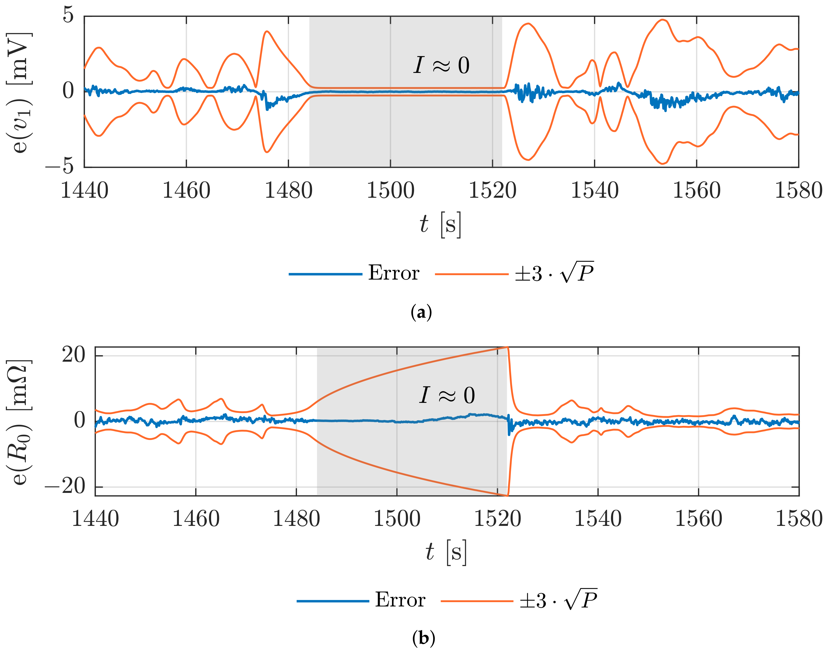
In phases, where the current becomes zero, the estimation of the polarization voltages is very good and the confidence interval shrinks significantly. As an example, Figure 8a emphasizes this in the gray area for the time s until s. This can be explained by considering the behavior of the polarization voltages when the current becomes zero. From a certain point in time , when the current becomes zero, the progression of the polarization voltages can be modeled as follows:
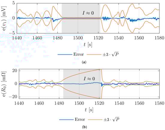
Figure 8.
Zoomed illustration of the estimation error (blue) and the corresponding bound (orange), when the current becomes zero for (a) the state and (b) the parameter .
With increasing time not only the polarization voltages, but also the slope will decrease. This leads to smaller entries in the linearized system matrix and to a decrease of the corresponding values in (see Algorithm 1).
In contrast, the parameters behave in opposite ways. When the current becomes zero, the confidence interval increases significantly, and the estimation cannot be trusted. As highlighted in Figure 8b, this is the case especially for . Without current flow, the input u is also zero and the parameters do not have any influence on the measured terminal voltage. Therefore, it is not possible to draw conclusions about the parameters (they are not observable), which leads to an increase of the confidence intervals.
4.2. Experimental Study
In the experimental study, the GA optimization converges after around 67 generations. However, when analyzing the resulting Pareto front in Figure 9, there is no clear trade-off visible between the three optimization objectives. It is not possible to reduce both consistency criteria at the same time. At least one is close to the upper limit of 0.5. Since the true state vector is not known and strongly depends on the simulated reference state vector, this criterion should not be over-rated. A closer examination of the model error reveals an RMSE of mV indicating errors in the state vector and therefore results in errors when calculating and . Hence, a lower value should be preferred over a low .
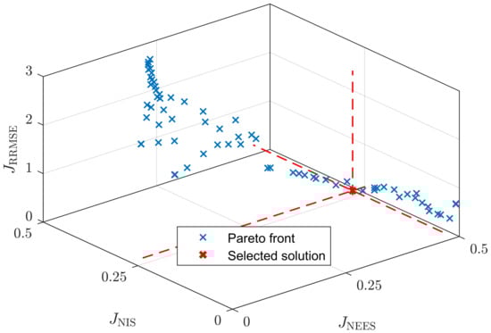
Figure 9.
Pareto front (blue) and the selected solution (red) in the objective space for the experimental case.
As in the simulative study, the solution with the smallest euclidean distance in the objective space is chosen as the most suitable solution. This leads to a very high of 0.46 with , , and the process noise is
In comparison to the simulative study, all optimization objectives are worse, and the process noise entries corresponding to the polarization voltages increase significantly due to inaccuracies of the proposed model. The validation results in Figure 10 based on the UDDS cycle show similar values for the fitness functions (, and ) and hence prove the feasibility of the procedure. The RMSE value is for the SOC , mV, mV, , and . All errors are reasonably small and the confidence intervals are in the same order of magnitude. For example, Wang et al. [13] achieved an RMSE of less than 1.5% for SOC using a Dual Sigma point Kalman filter that is also tuned with GA, but no values for other states and parameters or consistency are reported. Ref. [33] archived an RMSE of 1.9% for the SOC with an augmented unscented Kalman filter. Furthermore, when the current becomes zero, the estimator has a similar behavior as in the simulative study.
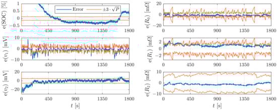
Figure 10.
Illustration of the error (blue) of the states and parameters with the corresponding bound (orange) in the experimental study using the UDDS cycle.
The experimental results demonstrate applicability with a considerable high computational effort. However, the large optimization space becomes a manageable set of optimal Pareto solutions decreasing significantly the required hands-on work of an experienced application engineer.
5. Conclusions
Determining the process noise of a KF algorithm appropriately is difficult and a very time consuming task without a suitable procedure. Hence, a traceable offline optimization procedure was developed to parametrize an EKF. It uses a multi-objective GA not only to minimize the estimation error, but also to design a consistent filter, which leads to a comprehensible set of optimal Pareto solutions. For identifying the consistency, the NEES and NIS distribution were evaluated. In this contribution, the procedure was applied to an EKF, which estimates the states and parameters of an NCA/graphite lithium-ion cell type. While the simulative data shows a good trade-off between the specified objectives, in the experimental case the NEES consistency measure must be neglected, since the reference data are subject to errors. Even in the experimental case, considerable small errors were archived with a suitable estimated covariance. This proceeding helps to determine the process noise in a convenient and comparable way. The conducted studies show the feasibility of the proposed methodology with a one time offline computational effort.
Author Contributions
M.T. Methodology, Software, Investigation, Validation, Writing—Original Draft. D.S. Conceptualization, Methodology, Investigation, Validation, Writing—Original Draft, Writing—Review and Editing. C.E. Funding acquisition, Supervision, Project administration, Writing—Review and Editing. All authors have read and agreed to the published version of the manuscript.
Funding
This work was funded by the AUDI AG within the scope of an ongoing research project. Furthermore, we acknowledge support by the Open Access Publication Fund of Technische Hochschulen Ingolstadt.
Institutional Review Board Statement
Not applicable.
Informed Consent Statement
Not applicable.
Data Availability Statement
Not applicable.
Acknowledgments
Special thanks are given to the support by M. Lewerenz for revising this work and M. Hinterberger for valuable discussions. Additionally, we thank C. Hartmann und C. Hanzl for providing software and developing hardware components, which were used for the experimental investigation.
Conflicts of Interest
The authors declare no conflict of interest.
References
- Shrivastava, P.; Soon, T.K.; Idris, M.Y.I.B.; Mekhilef, S. Overview of model-based online state-of-charge estimation using Kalman filter family for lithium-ion batteries. Renew. Sustain. Energy Rev. 2019, 113, 109233. [Google Scholar] [CrossRef]
- Mehra, R. Approaches to adaptive filtering. IEEE Trans. Autom. Control 1972, 17, 693–698. [Google Scholar] [CrossRef]
- Matisko, P.; Havlena, V. Noise covariance estimation for Kalman filter tuning using Bayesian approach and Monte Carlo. Int. J. Adapt. Control Signal Process. 2013, 27, 957–973. [Google Scholar] [CrossRef]
- Zagrobelny, M.A.; Rawlings, J.B. Identification of Disturbance Covariances Using Maximum Likelihood Estimation. TWCCC. 2014. Available online: https://engineering.ucsb.edu/~jbraw/jbrweb-archives/tech-reports/twccc-2014-02.pdf (accessed on 18 August 2012).
- Belanger, P.R. Estimation of Noise Covariance Matrices for a Linear Time-Varying Stochastic Process. IFAC Proc. Vol. 1972, 5, 265–271. [Google Scholar] [CrossRef]
- Åkesson, B.M.; Jørgensen, J.B.; Poulsen, N.K.; Jørgensen, S.B. A generalized autocovariance least-squares method for Kalman filter tuning. J. Process Control 2008, 18, 769–779. [Google Scholar] [CrossRef]
- Bohlin, T. Four Cases of Identification of Changing Systems. Math. Sci. Eng. 1976, 126, 441–518. [Google Scholar] [CrossRef]
- Mohamed, A.H.; Schwarz, K.P. Adaptive Kalman Filtering for INS/GPS. J. Geod. 1999, 73, 193–203. [Google Scholar] [CrossRef]
- Wang, J. Stochastic Modeling for Real-Time Kinematic GPS/GLONASS Positioning. Navigation 1999, 46, 297–305. [Google Scholar] [CrossRef]
- Dreano, D.; Tandeo, P.; Pulido, M.; Ait-El-Fquih, B.; Chonavel, T.; Hoteit, I. Estimating model-error covariances in nonlinear state-space models using Kalman smoothing and the expectation-maximization algorithm. Q. J. R. Meteorol. Soc. 2017, 143, 1877–1885. [Google Scholar] [CrossRef]
- Odelson, B.J.; Rajamani, M.R.; Rawlings, J.B. A new autocovariance least-squares method for estimating noise covariances. Automatica 2006, 42, 303–308. [Google Scholar] [CrossRef]
- Rayyam, M.; Zazi, M. Particle Swarm optimization of a Non-Linear Kalman Filter for Sensorles Control of Induction Motors. In Proceedings of the 2018 7th International Conference on Renewable Energy Research and Applications (ICRERA), Paris, France, 14–17 October 2018; pp. 1016–1020. [Google Scholar] [CrossRef]
- Wang, Z.; Gladwin, D.T.; Smith, M.J.; Haass, S. Practical state estimation using Kalman filter methods for large-scale battery systems. Appl. Energy 2021, 294, 117022. [Google Scholar] [CrossRef]
- Ting, T.O.; Man, K.L.; Lim, E.G.; Leach, M. Tuning of Kalman filter parameters via genetic algorithm for state-of-charge estimation in battery management system. Sci. World J. 2014, 2014, 176052. [Google Scholar] [CrossRef]
- Yang, R.; Xiong, R.; He, H.; Mu, H.; Wang, C. A novel method on estimating the degradation and state of charge of lithium-ion batteries used for electrical vehicles. Appl. Energy 2017, 207, 336–345. [Google Scholar] [CrossRef]
- Oshman, Y.; Shaviv, I. Optimal tuning of a Kalman filter using genetic algorithms. In Proceedings of the AIAA Guidance, Navigation, and Control Conference and Exhibit, Denver, CO, USA, 14–17 August 2000; American Institute of Aeronautics and Astronautics: Reston, VA, USA, 2000. [Google Scholar] [CrossRef]
- Goldberg, D.E. Genetic Algorithms in Search, Optimization, and Machine Learning; Addison-Wesley: Boston, MA, USA, 1989. [Google Scholar]
- Nejad, S.; Gladwin, D.T.; Stone, D.A. Sensitivity of lumped parameter battery models to constituent parallel-RC element parameterisation error. In Proceedings of the IECON 2014—40th Annual Conference of the IEEE Industrial Electronics Society, Dallas, TX, USA, 29 October—1 November 2014; pp. 5660–5665. [Google Scholar] [CrossRef]
- He, Y.; Liu, W.; Koch, B.J. Battery algorithm verification and development using hardware-in-the-loop testing. J. Power Sources 2010, 195, 2969–2974. [Google Scholar] [CrossRef]
- Ouyang, M.; Liu, G.; Lu, L.; Li, J.; Han, X. Enhancing the estimation accuracy in low state-of-charge area: A novel onboard battery model through surface state of charge determination. J. Power Sources 2014, 270, 221–237. [Google Scholar] [CrossRef]
- Hu, X.; Li, S.; Peng, H. A comparative study of equivalent circuit models for Li-ion batteries. J. Power Sources 2012, 198, 359–367. [Google Scholar] [CrossRef]
- Nejad, S.; Gladwin, D.T.; Stone, D.A. A systematic review of lumped-parameter equivalent circuit models for real-time estimation of lithium-ion battery states. J. Power Sources 2016, 316, 183–196. [Google Scholar] [CrossRef]
- Wang, Q.; Wang, J.; Zhao, P.; Kang, J.; Yan, F.; Du, C. Correlation between the model accuracy and model-based SOC estimation. Electrochim. Acta 2017, 228, 146–159. [Google Scholar] [CrossRef]
- Schneider, D.; Liebhart, B.; Endisch, C. Active state and parameter estimation as part of intelligent battery systems. J. Energy Storage 2021, 39, 102638. [Google Scholar] [CrossRef]
- Kalman, R.E. A New Approach to Linear Filtering and Prediction Problems. J. Basic Eng. 1960, 82, 35–45. [Google Scholar] [CrossRef]
- Yang, J.; Xia, B.; Shang, Y.; Huang, W.; Mi, C.C. Adaptive State-of-Charge Estimation Based on a Split Battery Model for Electric Vehicle Applications. IEEE Trans. Veh. Technol. 2017, 66, 10889–10898. [Google Scholar] [CrossRef]
- Deb, K. Multi-Objective Optimization Using Evolutionary Algorithms, 1st ed.; Wiley-Interscience Series in Systems and Optimization; Wiley: Chichester, UK, 2001. [Google Scholar]
- Bar-Shalom, Y.; Li, X.R.; Kirubarajan, T. Estimation with Applications to Tracking and Navigation: Theory Algorithms and Software; John Wiley & Sons, Inc.: New York, NY, USA, 2001. [Google Scholar] [CrossRef]
- Rothlauf, F. Representations for Genetic and Evolutionary Algorithms; Volume 104: Studies in Fuzziness and Soft Computing; Physica-Verlag Heidelberg: Heidelberg, Germany, 2002. [Google Scholar] [CrossRef]
- Brabazon, A.; O’Neill, M.; McGarraghy, S. Natural Computing Algorithms; Natural Computing Series; Springer: Berlin/Heidelberg, Germany, 2015. [Google Scholar]
- Genetic Algorithm Options (R2021b). 2021. Available online: https://de.mathworks.com/help/gads/genetic-algorithm-options.html (accessed on 3 January 2022).
- Deb, K.; Pratap, A.; Agarwal, S.; Meyarivan, T. A fast and elitist multiobjective genetic algorithm: NSGA-II. IEEE Trans. Evol. Comput. 2002, 6, 182–197. [Google Scholar] [CrossRef]
- Biswas, A.; Gu, R.; Kollmeyer, P.; Ahmed, R.; Emadi, A. Simultaneous State and Parameter Estimation of Li-Ion Battery With One State Hysteresis Model Using Augmented Unscented Kalman Filter. In Proceedings of the 2018 IEEE Transportation Electrification Conference and Expo (ITEC), Long Beach, CA, USA, 13–15 June 2018; pp. 1065–1070. [Google Scholar] [CrossRef]


Publisher’s Note: MDPI stays neutral with regard to jurisdictional claims in published maps and institutional affiliations. |
© 2022 by the authors. Licensee MDPI, Basel, Switzerland. This article is an open access article distributed under the terms and conditions of the Creative Commons Attribution (CC BY) license (https://creativecommons.org/licenses/by/4.0/).