
Evaluation of Focus Measures for Hyperspectral Imaging Microscopy Using Principal Component Analysis


Abstract
:1. Introduction
2. Materials and Methods
2.1. Autofocus Methods
2.2. The Focus Measures
- (i)
- Energy of Laplacian (EOL): This FM retrieves the sharpness value by analyzing high spatial frequencies associated with image borders and is computed by convolving an image with the convolution mask given bywhere and are the Laplacian operators.
- (ii)
- Sum-Modified Laplacian (SML): Proposed by Nayer and Nakagawa [34], this function serves as an alternative definition of EOL. It is derived from the observation that horizontal and vertical directions can have opposite signs, canceling each other out:
- (iii)
- Diagonal Laplacian (DLF): This focus measure, proposed by [35], extends the SML with diagonal terms, thus considering variations in both directions, i.e., along the spectral and spatial directions in hyperspectral images. It was subjected to evaluations in this work:where
- (iv)
- with parameters , and is named the Thresholded Absolute Gradient, and referred to as in this paper. The ABG is based on summing the first derivative of the image in the horizontal dimension, as a focused image has more gradients than a defocused image.
- (v)
- The case with parameters is named the Squared Absolute (). The is distinguished from the ABG y summing the square of the first derivative of the image in the horizontal dimension, to increase the contribution of larger gradients.
- (vi)
- The case with parameters is named the Brenner function (BRE) [32]. This focus measure (FM) is based on the second difference of the image intensity in the horizontal direction, which corresponds to the spatial axis of hyperspectral images. Some works also report applying it in the vertical direction.
- (vii)
- Energy of Image Gradient (EIG): This measure accumulates the sum of squared directional gradients, given by the following [36]:where , and
- (viii)
- Boddeke’s Algorithm (BOD): This function relies on computing a gradient magnitude value using a one-dimensional convolution mask, specifically along a single direction [27]. In the evaluations of hyperspectral image stacks, this direction corresponds to the spatial information dimension.where .
- (i)
- The Normalized Variance of an Image (NVR) is based on summing the variance of an image’s gray level with respect to its mean intensity and is defined asand here represents the mean intensity; W and H are the image width and height in pixels.
- (ii)
- The Autocorrelation Function (ACF), also known as Vollah’s F4 function, is more robust to image noise and computes the image’s autocorrelation [23]:
- (iii)
- The Standard Deviation-based Autocorrelation Function (Vollah’s F5 function) is utilized, which suppresses high frequencies (VOL5) [37]:
- (iv)
- Entropy Function (ENT): A focused image has higher entropy (i.e., more information) than a defocused image, and therefore, the range of the image histogram can be used as an FM. The ENT FM uses the image histogram and is defined aswhere is the probability for each intensity level in the histogram; represents the number of pixels with intensity .
- (v)
- Variance of the Log-histogram (LOG): This FM is based on the assumption that high-intensity pixels contribute to the upper part of the histogram and addresses the image’s brightness level through a logarithmic transformation of the histogram [23].where .
- (vi)
- Weighted Histogram (WHS): This FM is based on a weighted image histogram without introducing a constant threshold, taking into account that a focused image has more bright pixels than a defocused image [23]. The values of power and roots are determined empirically. Here, and represent the gray level and the number of pixels at each gray level, respectively.
- (i)
- The first is the Fourier transform (FFT), which is given byand here and are the coordinates in the frequency domain, and is the Fourier transform of the image, where the zero-frequency component is shifted to the center of the Fourier spectrum, i.e., the image array is first zero-padded before performing the FFT. From the real and imaginary parts of each transformed array, the value of the FM is calculated.
- (ii)
- The second transform-based FM is named as the Discrete Cosine Transform (DCT) was calculated using the formulahere if or if and in other cases.
- (iii)
- (iv)
- (WL1) Wavelet Algorithm: This FM sums the absolute values in sub-images:
- (v)
- (WL2) Wavelet Algorithm: This FM uses the variance of wavelet coefficients and sums them in sub-images. Here, the mean values μ in each region are computed from absolute values.
- (vi)
- (WL3) Wavelet Algorithm: The difference between WL2 and WL3 is that the mean values μ are computed without absolute values:
2.3. PCA
2.4. Ranking Criteria
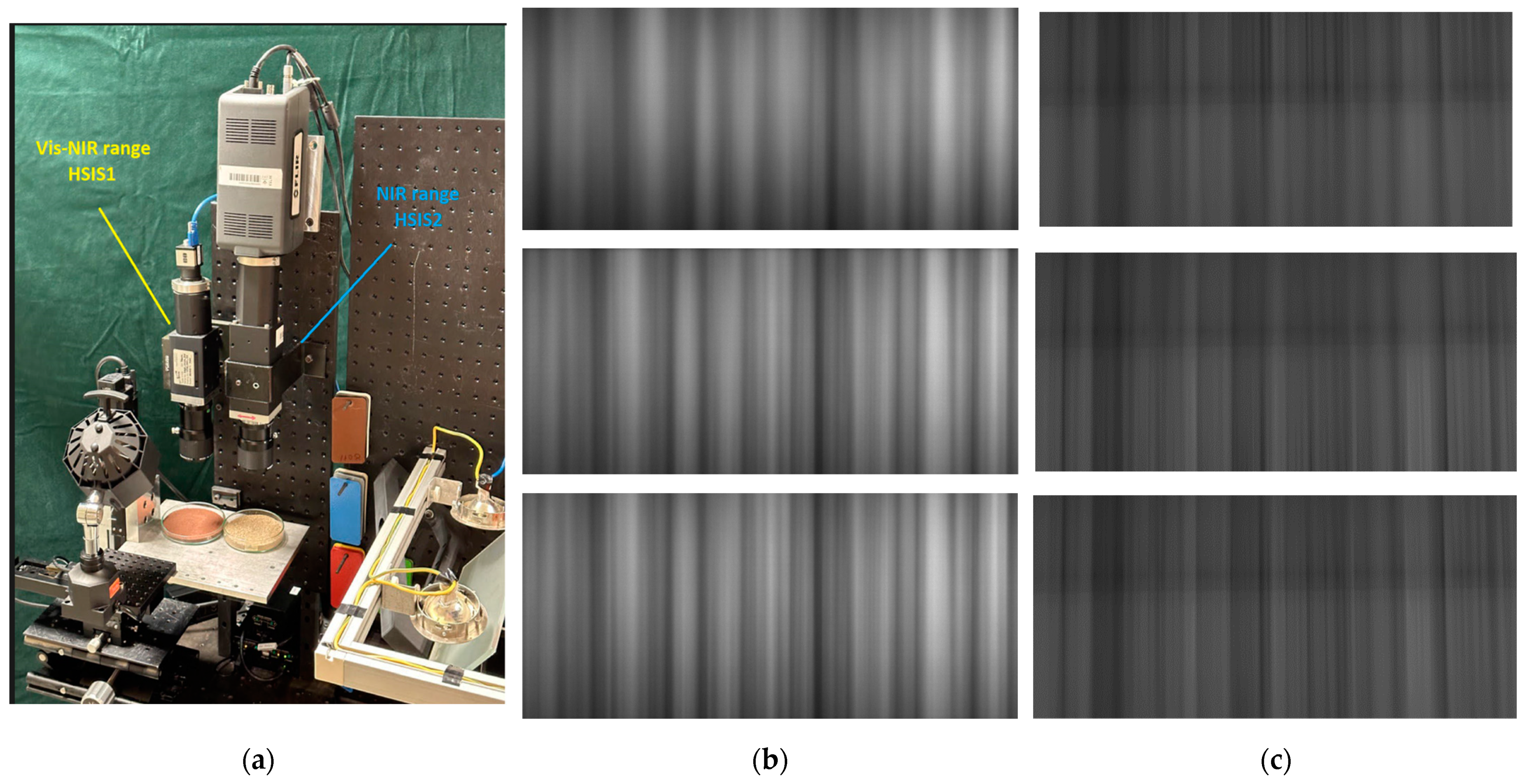
2.5. HSIMs
2.6. Instrument Calibration
2.7. Samples and Sample Preparation
2.8. Image Acquisition
3. Results
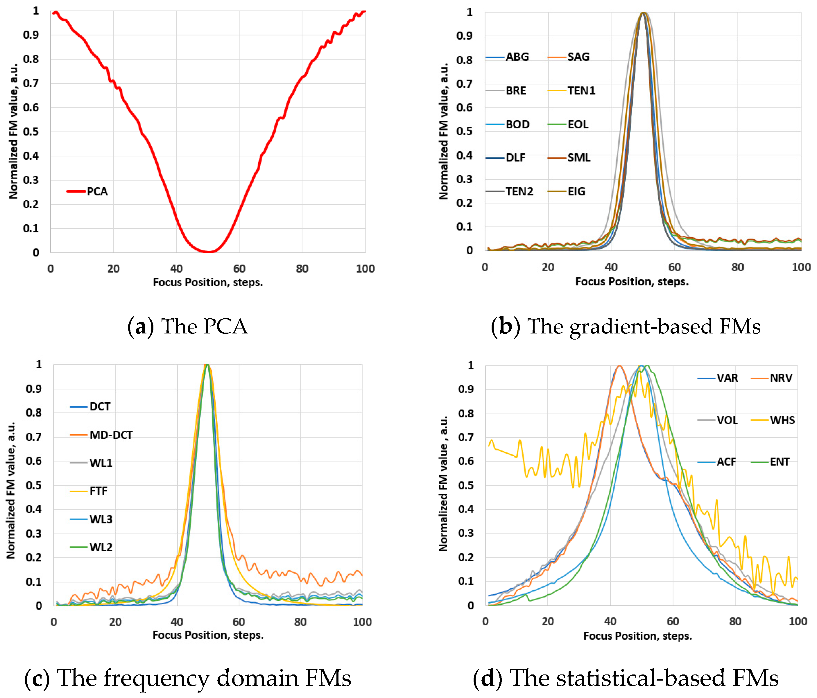
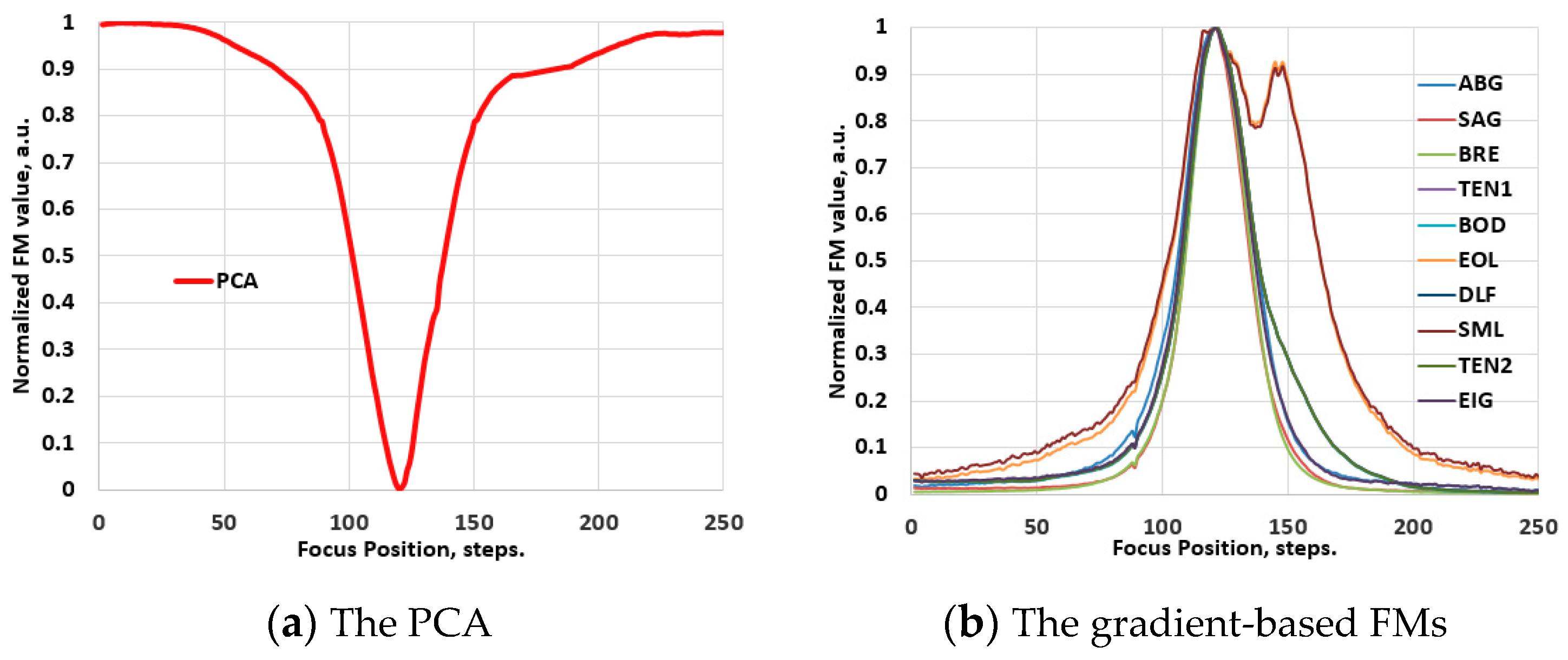
3.1. Validation Phase: Video Images
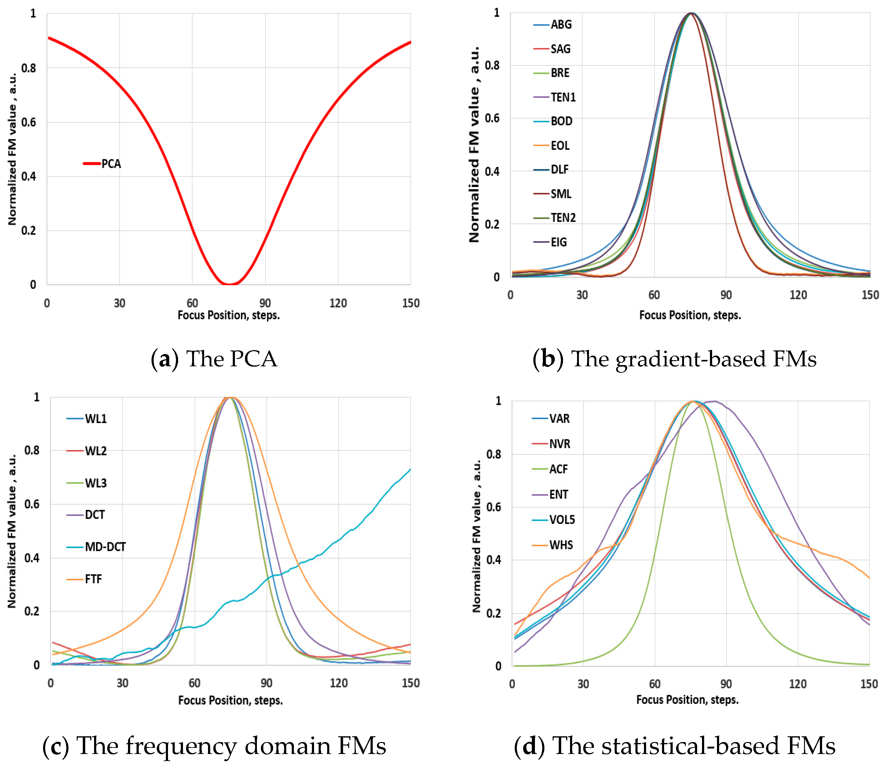
3.2. The Behavior of the FMs in Hyperspectral Images
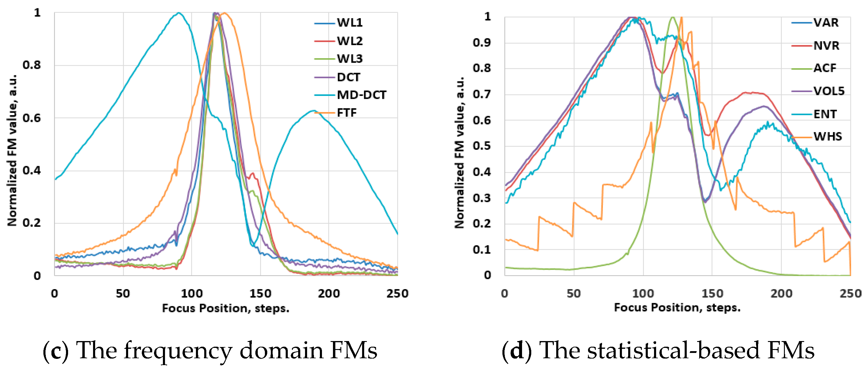
3.2.1. The Vis-NIR Range
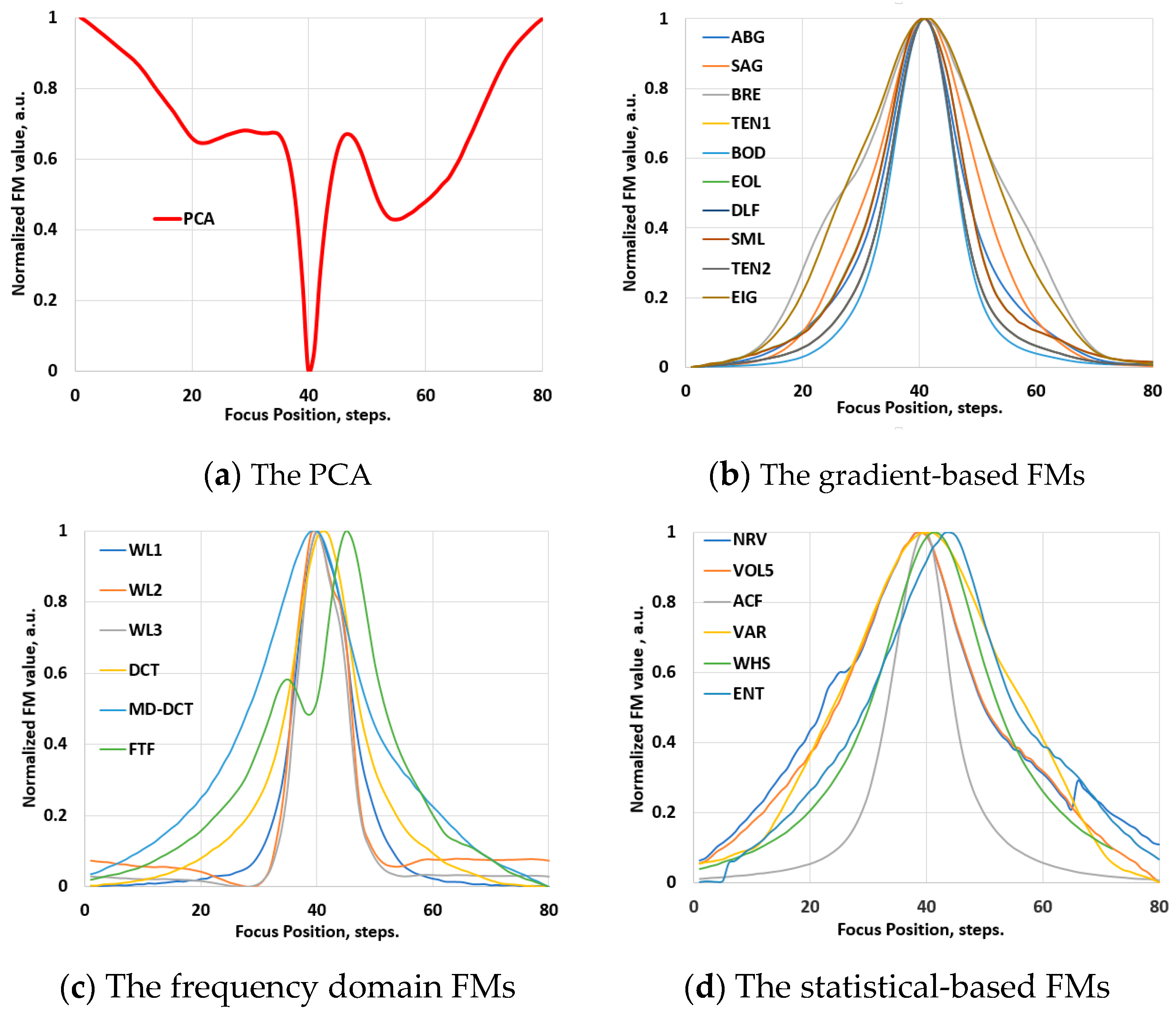
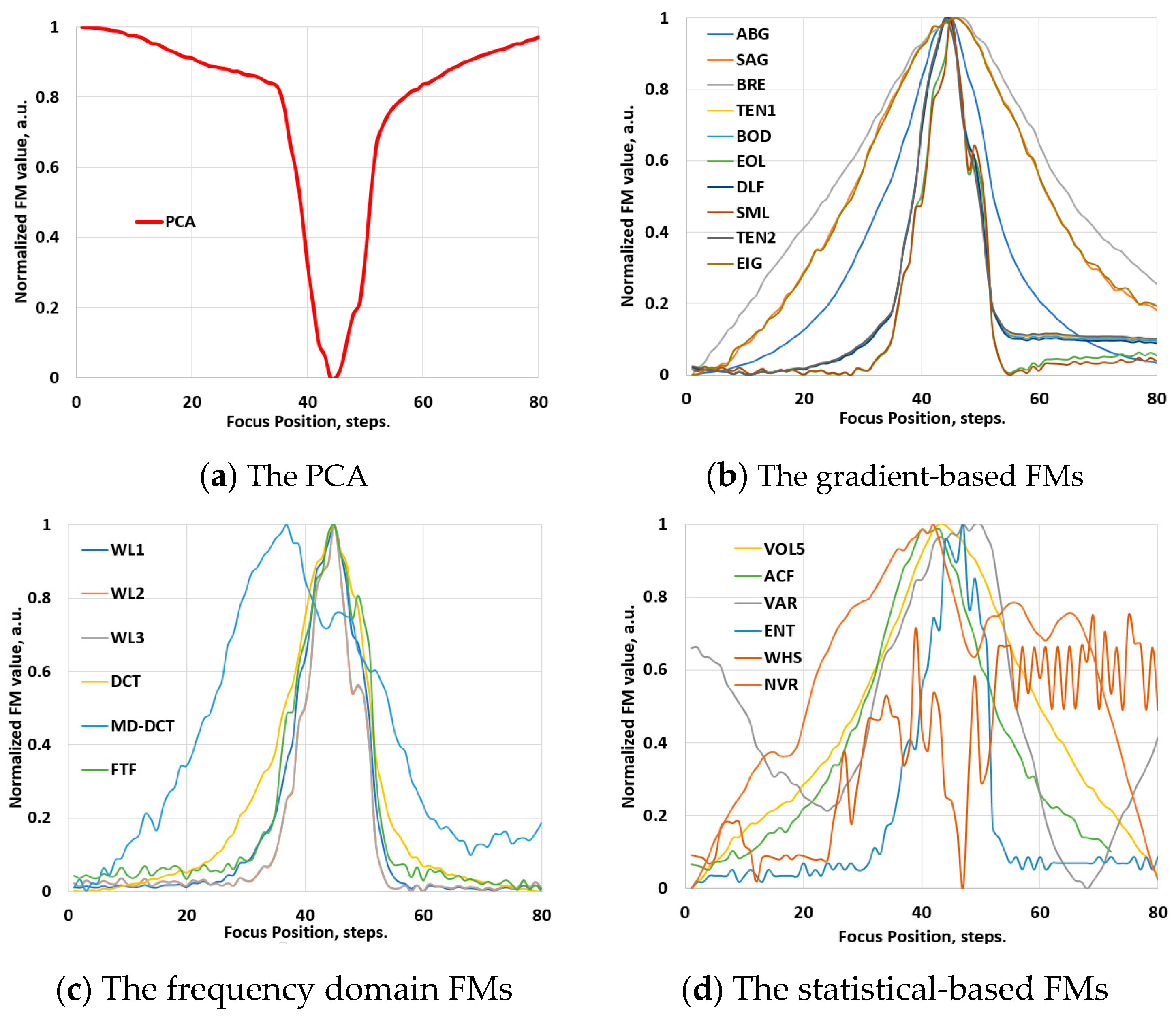
3.2.2. The NIR Range
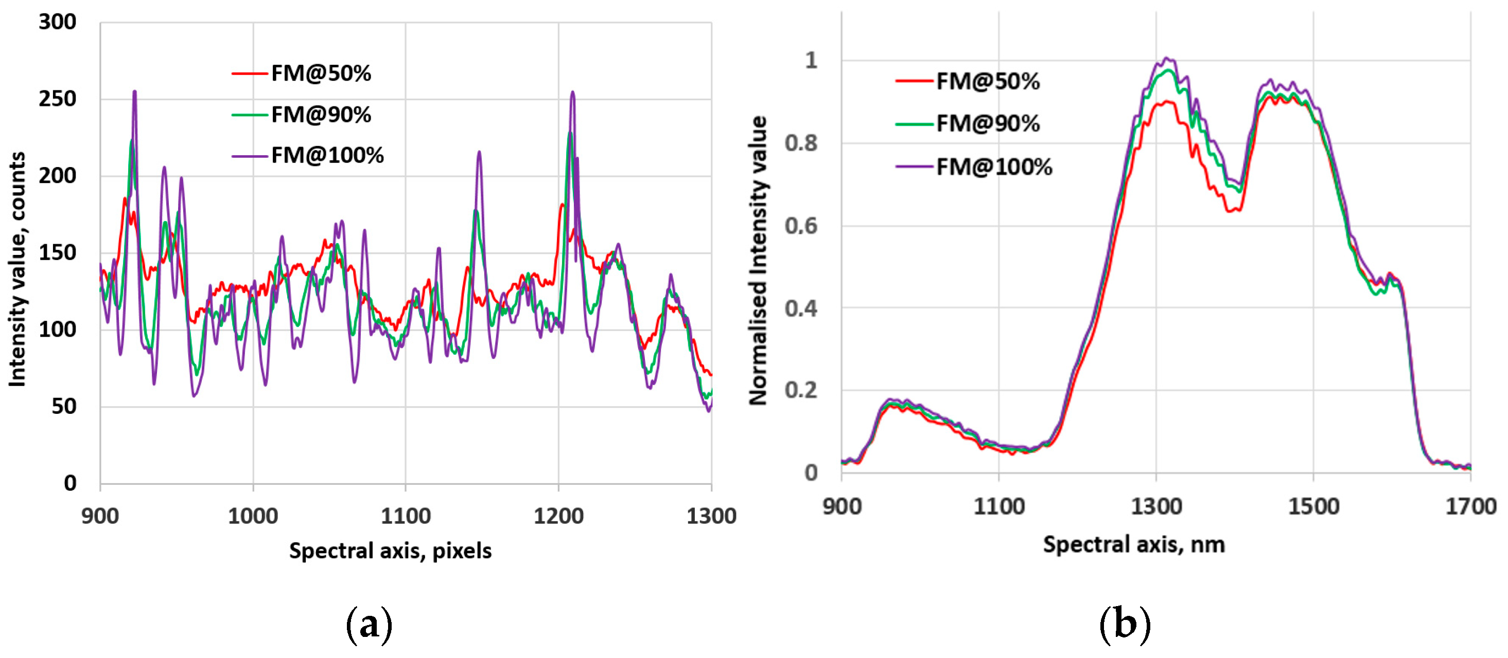
3.3. Robustness of the FMs
4. Discussion
4.1. Results of Ranking Evaluations
4.1.1. Ranking Evaluations for the Conventional Images
4.1.2. Ranking Evaluations for the Hyperspectral Images
5. Conclusions
Funding
Institutional Review Board Statement
Informed Consent Statement
Data Availability Statement
Acknowledgments
Conflicts of Interest
References
- Jong, L.; Kruif, N.; Geldof, F.; Veluponnar, D.; Sanders, J.; Peeters, M.-V.; Duijnhoven, F.; Sterenborg, H.; Dashtbozorg, B.; Ruers, T. Discriminating healthy from tumor tissue in breast lumpectomy specimens using deep learning-based hyperspectral imaging. Biomed. Opt. Express 2022, 13, 2581–2604. [Google Scholar] [CrossRef] [PubMed]
- Cinar, U.; Cetin Atalay, R.; Cetin, Y.Y. Human Hepatocellular Carcinoma Classification from H&E Stained Histopathology Images with 3D Convolutional Neural Networks and Focal Loss Function. J. Imaging 2023, 9, 25. [Google Scholar] [CrossRef] [PubMed]
- Riu, L.; Poulet, F.; Carter, J.; Bibring, J.-P.; Gondet, B.; Vincendon, M. The M3 project: 1-A global hyperspectral image-cube of the martian surface. Icarus 2019, 319, 281–292. [Google Scholar] [CrossRef]
- Kucheryavskiy, S. A new approach for discrimination of objects on hyperspectral images. Chemom. Intell. Lab. Syst. 2013, 120, 126–135. [Google Scholar] [CrossRef]
- Shi, P.; Jiang, Q.; Li, Z. Hyperspectral Characteristic Band Selection and Estimation Content of Soil Petroleum Hydrocarbon Based on GARF-PLSR. J. Imaging 2023, 9, 87. [Google Scholar] [CrossRef]
- Hao, J.; Zhang, Y.; Zhang, Y.; Wu, L. Prediction of antioxidant enzyme activity in tomato leaves based on microhyperspectral imaging technique. Opt. Laser Technol. 2024, 179, 111292. [Google Scholar] [CrossRef]
- Zander, P.D.; Wienhues, G.; Grosjean, M. Scanning Hyperspectral Imaging for In Situ Biogeochemical Analysis of Lake Sediment Cores: Review of Recent Developments. J. Imaging 2022, 8, 58. [Google Scholar] [CrossRef]
- Boldrini, B.; Kessler, W.; Rebner, K.; Kessler, R.-W. Hyperspectral imaging: A review of be practice, performance and pitfalls for in-line and on-line applications. J. Near Infrared Spectrosc. 2012, 20, 483–508. [Google Scholar] [CrossRef]
- Vohland, M.; Ludwig, M.; Thiele-Bruhn, S.; Ludwig, B. Quantification of Soil Properties with Hyperspectral Data: Selecting Spectral Variables with Different Methods to Improve Accuracies and Analyze Prediction Mechanisms. Remote Sens. 2017, 9, 1103. [Google Scholar] [CrossRef]
- Signoroni, A.; Savardi, M.; Baronio, A.; Benini, S. Deep Learning Meets Hyperspectral Image Analysis: A Multidisciplinary Review. J. Imaging 2019, 5, 52. [Google Scholar] [CrossRef]
- Gruber, F.; Wollmann, P.; Grählert, W.; Kaskel, S. Hyperspectral Imaging Using Laser Excitation for Fast Raman and Fluorescence Hyperspectral Imaging for Sorting and Quality Control Applications. J. Imaging 2018, 4, 110. [Google Scholar] [CrossRef]
- Hossain, M.; Younis, M.; Robinson, A.; Wang, L.; Preza, C. Greedy Ensemble Hyperspectral Anomaly Detection. J. Imaging 2024, 10, 131. [Google Scholar] [CrossRef] [PubMed]
- Zhu, M.; Huang, D.; Hu, X.-J.; Tong, W.-H.; Han, B.-L.; Tian, J.-P.; Luo, H.-B. Application of hyperspectral technology in detection of agricultural products and food: A Review. Food Sci. Nutr. 2020, 8, 5206–5214. [Google Scholar] [CrossRef] [PubMed]
- Temiz, H.-T.; Ulaş, B. A Review of Recent Studies Employing Hyperspectral Imaging for the Determination of Food Adulteration. Photochem 2021, 1, 125–146. [Google Scholar] [CrossRef]
- Lin, C.; Hu, Y.; Liu, Z.; Peng, Y.; Wang, L.; Peng, D. Estimation of Cultivated Land Quality Based on Soil Hyperspectral Data. Agriculture 2022, 12, 93. [Google Scholar] [CrossRef]
- Gosavi, D.; Cheatham, B.; Sztuba-Solinska, J. Label-Free Detection of Human Coronaviruses in Infected Cells Using Enhanced Darkfield Hyperspectral Microscopy (EDHM). J. Imaging 2022, 8, 24. [Google Scholar] [CrossRef]
- Zhang, J. A Hybrid Clustering Method with a Filter Feature Selection for Hyperspectral Image Classification. J. Imaging 2022, 8, 180. [Google Scholar] [CrossRef]
- Yazdanfar, S.; Kenny, K.-B.; Tasimi, K.; Corwin, A.-D.; Dixon, E.-L.; Filkins, R.-J. Simple and robust image-based autofocusing for digital microscopy. Opt. Express 2008, 16, 8670–8677. [Google Scholar] [CrossRef]
- Krotkov, E. Focusing. Int. J. Comput. Vis. 1988, 1, 223–237. [Google Scholar] [CrossRef]
- Sun, Y.; Duthaler, S.; Nelson, B.-J. Autofocusing in computer microscopy: Selecting the optimal focus algorithm. Microsc. Res. Tech. 2004, 65, 139–149. [Google Scholar] [CrossRef]
- Knapper, J.; Collins, J.-T.; Stirling, J.; McDermott, S.; Wadsworth, W.; Bowman, R.-W. Fast, high-precision autofocus on a motorised microscope: Automating blood sample imaging on the OpenFlexure Microscope. J. Microsc. 2022, 285, 29–39. [Google Scholar] [CrossRef] [PubMed]
- Liu, X.-A.; Wang, W.-A.; Sun, Y. Dynamic evaluation of autofocusing for automated microscopic analysis of blood smear and pap smear. J. Microsc. 2007, 227, 15–23. [Google Scholar] [CrossRef]
- Mateos-Pérez, J.-M.; Redondo, R.; Nava, R.; Valdiviezo, J.-C.; Cristóbal, G.; Escalante-Ramírez, B.; Ruiz-Serrano, M.-J.; Pascau, J.; Desco, M. Comparative evaluation of autofocus algorithms for a real-time system for automatic detection of Mycobacterium tuberculosis. Cytometry 2012, 81A, 213–221. [Google Scholar] [CrossRef]
- Zhang, C.; Jia, D.; Wu, N. Autofocus method based on multi regions of interest window for cervical smear images. Multimeded Tools Appl. 2022, 81, 18783–18805. [Google Scholar] [CrossRef]
- Panicker, R.-O.; Soman, B.; Saini, G.; Rajan, J. A Review of Automatic Methods Based on Image Processing Techniques for Tuberculosis Detection from Microscopic Sputum Smear Images. J. Med. Syst. 2016, 40, 17. [Google Scholar] [CrossRef]
- Li, J. Autofocus searching algorithm considering human visual system limitations. Opt. Eng. 2005, 44, 113201. [Google Scholar] [CrossRef]
- Sanz, M.-B.; Sánchez, F.-M.; Borromeo, S. An algorithm selection methodology for automated focusing in optical microscopy. Microsc. Res. Tech. 2022, 85, 1742–1756. [Google Scholar] [CrossRef]
- Liang, Q.; Qu, Y.-F. A texture–analysis–based design method for self-adaptive focus criterion function. J. Microsc. 2012, 246, 190–201. [Google Scholar] [CrossRef]
- Fonseca, E.; Fiadeiro, P.; Pereira, M.; Pinheiro, A. Comparative analysis of autofocus functions in digital in-line phase-shifting holography. Appl. Opt. 2016, 55, 7663–7674. [Google Scholar] [CrossRef]
- Faundez-Zanuy, M.; Mekyska, J.; Espinosa-Duró, V. On the focusing of thermal images. Pattern Recognit. Lett. 2019, 32, 1548–1557. [Google Scholar] [CrossRef]
- Chun, M.-G.; Kong, S.-G. Focusing in thermal imagery using morphological gradient operator. Pattern Recognit. Lett. 2014, 38, 20–25. [Google Scholar] [CrossRef]
- Rudnaya, M.-E.; Mattheij, R.-M.-M.; Maubach, J.-M.-L. Evaluating sharpness functions for automated scanning electron microscopy. J. Microsc. 2009, 240, 38–49. [Google Scholar] [CrossRef] [PubMed]
- Bueno-Ibarra, M.-A.; Alvarez-Borrego, J.; Acho, L.; Cha’vez-Sanchez, M.-C. Fast autofocus algorithm for automated microscopes. Opt. Eng. 2005, 44, 6. [Google Scholar] [CrossRef]
- Nayar, S.K.; Nakagawa, Y. Shape from focus. IEEE Trans. Pattern Anal. Mach. Intell. 1994, 16, 824–831. [Google Scholar] [CrossRef]
- Pertuz, S.; Puig, D.; Garcia, M.-A. Analysis of focus measure operators for shape-from-focus. Pattern Recognit. 2013, 46, 1415–1432. [Google Scholar] [CrossRef]
- Santos, A.; Ortiz de Solórzano, C.; Vaquero, J.J.; Peña, J.M.; Malpica, N.; del Pozo, F. Evaluation of autofocus functions in molecular cytogenetic analysis. J. Microsc. 1997, 188, 264–272. [Google Scholar] [CrossRef]
- Brazdilova, S.-L.; Kozubek, M. Information content analysis in automated microscopy imaging using an adaptive autofocus algorithm for multimodal functions. J. Microsc. 2009, 236, 194–202. [Google Scholar] [CrossRef]
- Shah, M.-I.; Mishra, S.; Rout, C. Establishment of hybridized focus measure functions as a universal method for autofocusing. J. Biomed. Opt. 2017, 22, 126004. [Google Scholar] [CrossRef]
- Wan, T.; Zhu, C.; Qin, Z. Multifocus image fusion based on robust principal component analysis. Pattern Recognit. Lett. 2013, 34, 1001–1008. [Google Scholar] [CrossRef]
- Wu, G.; Liu, Z.; Fang, E.; Yu, H. Reconstruction of spectral color information using weighted principle component analysis. Optik 2015, 126, 1249–1253. [Google Scholar] [CrossRef]
- Kang, X.; Xiang, X.; Li, S.; Benediktsson, J.-A. PCA-Based Edge-Preserving Features for Hyperspectral Image Classification. IEEE Trans. Geosci. Remote Sens. 2017, 55, 7140–7151. [Google Scholar] [CrossRef]
- Uddin, M.P.; Mamun, M.A.; Hossain, M.A. PCA-based feature reduction for hyperspectral remote sensing image classification. IETE Tech. Rev. 2021, 38, 377–396. [Google Scholar] [CrossRef]
- Moore, B.E.; Gao, C.; Nadakuditi, R.R. Panoramic Robust PCA for Foreground–Background Separation on Noisy, Free-Motion Camera Video. IEEE Trans. Comput. Imaging 2019, 5, 195–211. [Google Scholar] [CrossRef]
- Moeller, S.; Pisharady, P.K.; Ramanna, S.; Lenglet, C.; Wu, X.; Dowdle, L.; Yacoub, E.; Uğurbil, K.; Akçakaya, M. NOise reduction with DIstribution Corrected (NORDIC) PCA in dMRI with complex-valued parameter-free locally low-rank processing. NeuroImage 2021, 226, 117539. [Google Scholar] [CrossRef]
- MATLAB®. Available online: https://www.mathworks.com/ (accessed on 20 September 2024).
- Nasibov, H.; Kholmatov, A.; Hacizade, F. Investigation of autofocus algorithms for Vis-NIR and NIR hyperspectral imaging microscopes. In Proceedings of the NIR 2013—16th International Conference on Near Infrared Spectroscopy, La Grande-Motte, France, 2–7 June 2013; pp. 595–601. [Google Scholar]
- Peleg, M.; McClements, J. Measures of line jaggedness and their use in foods textural evaluation. Crit. Rev. Food Sci. Nutr. 1997, 37, 491–518. [Google Scholar] [CrossRef]
- Nouri, D.; Lucas, Y.; Treuillet, S. Calibration and test of a hyperspectral imaging prototype for intra-operative surgical assistance. In Proceedings of the SPIE 8676, Medical Imaging, Lake Buena Vista, FL, USA, 9–14 February 2013. [Google Scholar] [CrossRef]


| Setup | HISM1 | HISM2 | HSIS1 | HSIS2 |
|---|---|---|---|---|
| Spectral range | 400–1000 nm | 900–1700 nm | 400–1000 nm | 900–1700 nm |
| Entrance slit, width × height | 30 μm × 9.8 mm | 50 μm × 9.8 mm | 25 μm × 9.8 mm | 25 μm × 9.8 mm |
| Spectral resolution | 3.8 nm/pixel | 6.7 nm/pixel | 1.3 nm/pixel | 4.1 nm/pixel |
| Imaging array | Pixel Fly, PCO | XenIcs, XEVA-17, InGaAs | EO, DCC3240x | FLIR, A6261, InGaAs |
| Array resolution, pixels | 1024 × 1392 | 256 × 320 | 1280 × 1024 | 640 × 512 |
| Dynamic range | 14 bits | 12 bits | 12 bits | 14 bits |
| Magnification | 50× to 100× | 25× to 50× | 0.1× to 0.5× | 0.1× to 0.5× |
| FM | Accuracy | Unimodality | Width at 50% | Width at 90% | Smoothness | Overall Score | Ranking |
|---|---|---|---|---|---|---|---|
| TEN1 | 0.10 | 0.00 | 0.59 | 0.37 | 0.59 | 0.92 | 1 |
| BOD | 0.15 | 0.00 | 0.54 | 0.46 | 0.58 | 0.93 | 2 |
| TEN2 | 0.10 | 0.00 | 0.56 | 0.41 | 0.62 | 0.94 | 3 |
| BRE | 0.05 | 0.05 | 0.59 | 0.47 | 0.60 | 0.97 | 4 |
| ABG | 0.05 | 0.05 | 0.68 | 0.60 | 0.59 | 1.08 | 5 |
| SAG | 0.11 | 0.11 | 0.59 | 0.53 | 0.81 | 1.14 | 6 |
| EIG | 0.32 | 0.12 | 0.62 | 0.58 | 0.77 | 1.20 | 7 |
| SML | 0.59 | 0.33 | 0.78 | 0.81 | 0.87 | 1.57 | 8 |
| EOL | 0.20 | 1.00 | 0.67 | 0.70 | 1.00 | 1.73 | 9 |
| DLF | 1.00 | 0.45 | 1.00 | 1.00 | 0.75 | 1.94 | 10 |
| WL3 | 0.10 | 0.00 | 0.55 | 0.39 | 0.49 | 0.84 | 1 |
| WL2 | 0.21 | 0.19 | 0.57 | 0.47 | 0.51 | 0.94 | 2 |
| WL1 | 0.18 | 0.11 | 0.59 | 0.48 | 0.53 | 0.95 | 3 |
| FTF | 0.83 | 0.92 | 0.69 | 0.76 | 0.67 | 1.74 | 4 |
| DCT | 1.00 | 1.00 | 0.74 | 0.90 | 0.65 | 1.94 | 5 |
| MD-DCT | 0.79 | 0.71 | 1.00 | 1.00 | 1.00 | 2.03 | 6 |
| NVR | 0.41 | 0.45 | 0.43 | 0.31 | 0.71 | 1.08 | 1 |
| ENT | 0.31 | 0.40 | 0.50 | 0.48 | 0.75 | 1.14 | 2 |
| VOL5 | 0.40 | 0.40 | 0.61 | 0.59 | 0.85 | 1.33 | 3 |
| ACF | 0.51 | 0.55 | 0.69 | 0.55 | 0.71 | 1.36 | 4 |
| VAR | 0.46 | 0.60 | 0.85 | 0.77 | 0.78 | 1.58 | 5 |
| WHS | 1.00 | 1.00 | 1.00 | 1.00 | 0.92 | 2.20 | 6 |
| FM | Accuracy | Unimodality | Width at 50% | Width at 90% | Smoothness | Overall Score | Ranking |
|---|---|---|---|---|---|---|---|
| TEN1 | 0.30 | 0.02 | 0.55 | 0.45 | 0.50 | 0.92 | 1 |
| TEN2 | 0.21 | 0.06 | 0.61 | 0.59 | 0.45 | 0.99 | 2 |
| ABG | 0.23 | 0.02 | 0.78 | 0.56 | 0.49 | 1.10 | 3 |
| BRE | 0.58 | 0.07 | 0.59 | 0.52 | 0.59 | 1.14 | 4 |
| BOD | 0.51 | 0.04 | 0.67 | 0.61 | 0.51 | 1.16 | 5 |
| SAG | 0.62 | 0.14 | 0.69 | 0.73 | 0.61 | 1.34 | 6 |
| EIG | 0.42 | 0.32 | 0.82 | 0.88 | 0.67 | 1.47 | 7 |
| EOL | 0.73 | 0.32 | 0.96 | 0.78 | 1.00 | 1.78 | 8 |
| DLF | 1.00 | 0.91 | 0.87 | 0.93 | 0.85 | 2.04 | 9 |
| SML | 0.63 | 1.00 | 1.00 | 1.00 | 0.91 | 2.06 | 10 |
| WL3 | 0.33 | 0.12 | 0.50 | 0.48 | 0.59 | 0.98 | 1 |
| WL2 | 0.37 | 0.22 | 0.57 | 0.51 | 0.45 | 0.99 | 2 |
| WL1 | 0.41 | 0.32 | 0.75 | 0.65 | 0.59 | 1.27 | 3 |
| FTF | 0.63 | 0.32 | 0.96 | 0.87 | 0.67 | 1.62 | 4 |
| DCT | 0.85 | 1.00 | 0.87 | 0.93 | 0.95 | 2.06 | 5 |
| MD-DCT | 1.00 | 0.91 | 1.00 | 1.00 | 1.00 | 2.20 | 6 |
| VOL5 | 0.40 | 0.21 | 0.61 | 0.49 | 0.65 | 1.11 | 1 |
| ACF | 0.41 | 0.09 | 0.59 | 0.65 | 0.60 | 1.14 | 2 |
| ENT | 0.31 | 0.42 | 0.56 | 0.60 | 0.75 | 1.23 | 3 |
| NVR | 0.48 | 0.13 | 0.63 | 0.71 | 0.71 | 1.29 | 4 |
| VAR | 0.76 | 1.00 | 0.85 | 0.77 | 1.00 | 1.97 | 5 |
| WHS | 1.00 | 0.96 | 1.00 | 1.00 | 0.91 | 2.18 | 6 |
| FM | Accuracy | Unimodality | Width at 50% | Width at 90% | Smoothness | Overall Score | Ranking |
|---|---|---|---|---|---|---|---|
| BRE | 0.19 | 0.07 | 0.39 | 0.35 | 0.30 | 0.64 | 1 |
| BOD | 0.21 | 0.10 | 0.37 | 0.35 | 0.35 | 0.66 | 2 |
| EIG | 0.30 | 0.12 | 0.32 | 0.38 | 0.32 | 0.67 | 3 |
| SAG | 0.29 | 0.14 | 0.29 | 0.33 | 0.41 | 0.68 | 4 |
| TEN1 | 0.23 | 0.08 | 0.45 | 0.36 | 0.31 | 0.70 | 5 |
| TEN2 | 0.21 | 0.09 | 0.41 | 0.32 | 0.42 | 0.71 | 6 |
| ABG | 0.29 | 0.11 | 0.37 | 0.40 | 0.49 | 0.80 | 7 |
| DLF | 0.67 | 0.45 | 0.87 | 0.93 | 0.55 | 1.60 | 8 |
| EOL | 1.00 | 1.00 | 1.00 | 0.88 | 1.00 | 2.19 | 9 |
| SML | 0.93 | 1.00 | 1.00 | 1.00 | 0.97 | 2.19 | 10 |
| WL3 | 0.23 | 0.08 | 0.38 | 0.35 | 0.31 | 0.65 | 1 |
| WL2 | 0.24 | 0.12 | 0.39 | 0.41 | 0.31 | 0.70 | 2 |
| WL1 | 0.27 | 0.12 | 0.41 | 0.43 | 0.34 | 0.75 | 3 |
| FTF | 0.53 | 1.00 | 1.00 | 0.87 | 0.67 | 1.87 | 4 |
| DCT | 0.75 | 0.90 | 0.81 | 1.00 | 0.95 | 1.98 | 5 |
| MD-DCT | 1.00 | 0.91 | 0.93 | 1.00 | 1.00 | 2.17 | 6 |
| ACF | 0.41 | 0.20 | 0.33 | 0.34 | 0.25 | 0.70 | 1 |
| VOL5 | 0.45 | 0.31 | 0.61 | 0.59 | 0.36 | 1.07 | 2 |
| ENT | 0.41 | 0.32 | 0.68 | 0.56 | 0.45 | 1.12 | 3 |
| VAR | 1.00 | 0.43 | 1.00 | 0.67 | 0.71 | 1.77 | 4 |
| NVR | 0.94 | 0.37 | 0.91 | 1.00 | 0.79 | 1.86 | 5 |
| WHS | 0.80 | 1.00 | 0.83 | 0.81 | 1.00 | 2.00 | 6 |
| FM | Accuracy | Unimodality | Width at 50% | Width at 90% | Smoothness | Overall Score | Ranking |
|---|---|---|---|---|---|---|---|
| BOD | 0.05 | 0.04 | 0.37 | 0.35 | 0.51 | 0.72 | 1 |
| TEN1 | 0.15 | 0.02 | 0.60 | 0.52 | 0.50 | 0.95 | 2 |
| TEN2 | 0.25 | 0.02 | 0.64 | 0.58 | 0.45 | 1.01 | 3 |
| ABG | 0.10 | 0.02 | 0.70 | 0.62 | 0.49 | 1.06 | 4 |
| BRE | 0.19 | 0.07 | 0.61 | 0.68 | 0.59 | 1.11 | 5 |
| SAG | 0.52 | 0.24 | 0.59 | 0.60 | 0.61 | 1.19 | 6 |
| EIG | 0.32 | 0.38 | 0.42 | 0.43 | 1.00 | 1.27 | 7 |
| SML | 1.00 | 0.80 | 0.50 | 0.55 | 0.71 | 1.64 | 8 |
| DLF | 0.64 | 0.71 | 0.66 | 0.93 | 0.86 | 1.72 | 9 |
| EOL | 0.73 | 1.00 | 1.00 | 1.00 | 0.85 | 2.06 | 10 |
| WL3 | 0.13 | 0.12 | 0.50 | 0.47 | 0.40 | 0.81 | 1 |
| WL2 | 0.16 | 0.12 | 0.59 | 0.56 | 0.45 | 0.95 | 2 |
| WL1 | 0.31 | 0.32 | 0.62 | 0.63 | 0.57 | 1.14 | 3 |
| FTF | 1.00 | 1.00 | 0.86 | 0.87 | 1.00 | 2.12 | 4 |
| DCT | 0.85 | 0.90 | 0.67 | 0.73 | 0.70 | 1.73 | 5 |
| MD-DCT | 1.00 | 0.80 | 1.00 | 1.00 | 0.88 | 2.10 | 6 |
| NVR | 0.44 | 0.23 | 0.59 | 0.57 | 0.41 | 1.04 | 1 |
| ENT | 0.49 | 0.12 | 0.61 | 0.60 | 0.35 | 1.05 | 2 |
| ACF | 0.57 | 0.31 | 0.60 | 0.55 | 0.68 | 1.24 | 3 |
| VOL5 | 0.65 | 0.29 | 0.71 | 0.60 | 0.63 | 1.33 | 4 |
| VAR | 1.00 | 1.00 | 0.85 | 0.86 | 0.83 | 2.04 | 5 |
| WHS | 0.91 | 0.80 | 1.00 | 1.00 | 1.00 | 2.11 | 6 |
Disclaimer/Publisher’s Note: The statements, opinions and data contained in all publications are solely those of the individual author(s) and contributor(s) and not of MDPI and/or the editor(s). MDPI and/or the editor(s) disclaim responsibility for any injury to people or property resulting from any ideas, methods, instructions or products referred to in the content. |
© 2024 by the author. Licensee MDPI, Basel, Switzerland. This article is an open access article distributed under the terms and conditions of the Creative Commons Attribution (CC BY) license (https://creativecommons.org/licenses/by/4.0/).
Share and Cite
Nasibov, H. Evaluation of Focus Measures for Hyperspectral Imaging Microscopy Using Principal Component Analysis. J. Imaging 2024, 10, 240. https://doi.org/10.3390/jimaging10100240
Nasibov H. Evaluation of Focus Measures for Hyperspectral Imaging Microscopy Using Principal Component Analysis. Journal of Imaging. 2024; 10(10):240. https://doi.org/10.3390/jimaging10100240
Chicago/Turabian StyleNasibov, Humbat. 2024. "Evaluation of Focus Measures for Hyperspectral Imaging Microscopy Using Principal Component Analysis" Journal of Imaging 10, no. 10: 240. https://doi.org/10.3390/jimaging10100240
APA StyleNasibov, H. (2024). Evaluation of Focus Measures for Hyperspectral Imaging Microscopy Using Principal Component Analysis. Journal of Imaging, 10(10), 240. https://doi.org/10.3390/jimaging10100240