Estimation Methods of the Point Spread Function Axial Position: A Comparative Computational Study

Abstract

The precise knowledge of the point spread function is central for any imaging system characterization. In fluorescence microscopy, point spread function (PSF) determination has become a common and obligatory task for each new experimental device, mainly due to its strong dependence on acquisition conditions. During the last decade, algorithms have been developed for the precise calculation of the PSF, which fit model parameters that describe image formation on the microscope to experimental data. In order to contribute to this subject, a comparative study of three parameter estimation methods is reported, namely: I-divergence minimization (MIDIV), maximum likelihood (ML) and non-linear least square (LSQR). They were applied to the estimation of the point source position on the optical axis, using a physical model. Methods’ performance was evaluated under different conditions and noise levels using synthetic images and considering success percentage, iteration number, computation time, accuracy and precision. The main results showed that the axial position estimation requires a high SNR to achieve an acceptable success level and higher still to be close to the estimation error lower bound. ML achieved a higher success percentage at lower SNR compared to MIDIV and LSQR with an intrinsic noise source. Only the ML and MIDIV methods achieved the error lower bound, but only with data belonging to the optical axis and high SNR. Extrinsic noise sources worsened the success percentage, but no difference was found between noise sources for the same method for all methods studied.

1. Introduction

The point spread function (PSF) is the image of a point source of light and the basic unit that makes up any image ([1], Chapter 14.4.1, pp. 335–337). Its precise knowledge is fundamental for the characterization of any imaging system, as well as for obtaining reliable results in applications like deconvolution [2], object localization [3] or superresolution imaging [4,5], to mention some. In conventional fluorescence microscopy, PSF determination has become a common task, due to its strong dependence on acquisition conditions. From its acquaintance, it is possible to determine instrument capacities to resolve details, restore out of focus information, and so forth. However, it is always restricted to a bounded and specific set of acquisition conditions. In fact, in optical sectioning microscopy, the three-dimensional (3D) PSF presents a significant spatial variance along the optical axis as a consequence of the aberrations introduced by the technique. Therefore, a single 3D PSF determination is not enough for a complete description of the system.

The PSF can be determined in three ways, namely experimental, theoretical or analytical ([1], Chapter 14.4.1, pp. 335–337) [6]. In the experimental approach, fluorescent sub-resolution microspheres are used for this purpose. The microsphere images must be acquired under the same conditions in which the specimen is registered. This is methodologically difficult to do, and the experimental PSFs just represent a portion of the whole space. However, it has the advantage of generating a more realistic PSF, evidencing aberrations that are difficult to model. The theoretical determination, in turn, responds to a set of mathematical equations that describe the physical model of the optics. The model’s parameter values are filled with the instrument data-sheet and the capture conditions. The modeling of certain aberrations and the absence of noise are its main advantages. The third way to determine PSF was originated from parametric blind deconvolution algorithms; it has the advantage of estimating the model parameters from real data, but its main application has been image restoration.

Along the last decade, alternative ways of 3D PSF determination have appeared because of the emergence of new applications in optical microscopy (e.g., localization microscopy; see recent review articles [3,7,8]). In a certain sense, these forms are similar to the PSF estimation by blind parametric deconvolution, since they fit a parametric model to an experimental 3D PSF. The contributions in this field are mainly represented by the works carried out by Hanser et al. [9], Aguet et al. [10], Mortensen et al. [11] and Kirshner et al. [12] and are aimed at connecting the physical formulation of the image formation and the experimental PSF. Hanser et al. [9] developed a methodology to estimate the microscopy parameters using recovery algorithms of the phase pupil function from experimental 3D PSF. Meanwhile, Aguet et al. [10] and Kirshner et al. [12] contributed with algorithms to estimate the 3D PSF parameters of the Gibson and Lanni theoretical model [13] from real data. Furthermore, Aguet et al. [10] investigated the feasibility of particle localization, from blurred sections, analyzing the Cramer–Rao theoretical lower bound.

Regarding parameter estimation method comparison applied to optical microscopy, one of the first method comparison studies was made by Cheezum et al. [14], who quantitatively compared the performance of four commonly-used methods for particle tracking problems: cross-correlation, sum-absolute difference, centroid and direct Gaussian fit. They found that the cross-correlation algorithm method was the most accurate for large particles, and for smaller point sources, direct Gaussian fit to the intensity distribution was superior in terms of both accuracy and precision, as well as robustness at a low signal-to-noise ratio (SNR). Abraham et al. [15] studied comparatively the performance of maximum likelihood and non-linear least square estimation methods for fitting single molecule data under different scenarios. Their results showed that both estimators, on average, are able to recover the true planar location of the single molecule, in all the scenarios they examined. In particular, they found that under model misspecifications and low noise levels, maximum likelihood is more precise than the non-linear least square method. Abraham et al. [15] used Gaussian and Airy profiles to model the PSF and to study the effect of pixelation on the results of the estimation methods.

All of these have been important advances in the research and development of tools for the precise determination of the PSF. However, according to the available literature, just a few ways of parameter estimation methods for theoretical PSF have been developed and, to our knowledge, there have been no comparative studies analyzing methods for parameter estimation of a more realistic PSF physical model. Thus, to contribute in this regard, in this article, a comparative computational study of three methods of 3D PSF parameter estimation of a wide-field fluorescence microscope is described. These were applied to improve the precision of the position on the optical axis of a point source using the model developed by Gibson and Lanni [13]. This parameter was selected because of its importance in applications such as depth-variant deconvolution [16,17] and localization microscopy [3,7], which is also an unknown parameter in a variant and non-linear image formation physical model.

The method comparison described in this report is based on sampling theory statistics, although it had not been devised in this way. Thus, it is essential to mention that there are several analyses based on the Bayesian paradigm of image interpretation. Shaevitz [18] developed an algorithm to localize a particle in the axial direction, which is also compared with other previously-developed methods that account for the PSF axial asymmetry. Rees et al. [19] analyzed the resolution achieved in localization microscopy experiments, and they highlighted the importance of assessing the resolution directly from the image samples by analyzing their particular datasets, which can significantly differ from the resolution evaluated from a calibration sample. De Santis et al. [5] obtained a precision expression for axial localization based on standard deviation measurements of the PSF intensity profile fitted to a Gaussian profile. Finally, a specific application can be found in the works of Cox et al. [20] and Walde et al. [21], who used the Bayesian approach for revealing the podosome biodynamics.

The remainder of this report is organized as follows. First, a description of the physical PSF model is presented; next, three forms of 3D PSF parameter estimation are shown, namely Csiszár I-divergence minimization (our own preceding development), maximum likelihood [10] and least square [12]. Since all expressions to optimize are of a non-linear nature, they are approximated using the same series representation, obtaining three iterative algorithms that differ in the comparison criteria between the data and the model. Following, in the Results Section, the performance of the algorithms has been extensively analyzed using synthetic data generated with different sources and noise levels. This was carried out evaluating: success percentage, number of iterations, computation time, accuracy and precision. As an application, the position on the optical axis of an experimental 3D PSF is estimated by the three methods, taking the difference between the full width at half maximum (FWHM) between the estimated and experimental 3D PSF as the comparison criterion. Results are analyzed in the Discussion Section. Finally, the main conclusions of this research are presented.

2. PSF Model

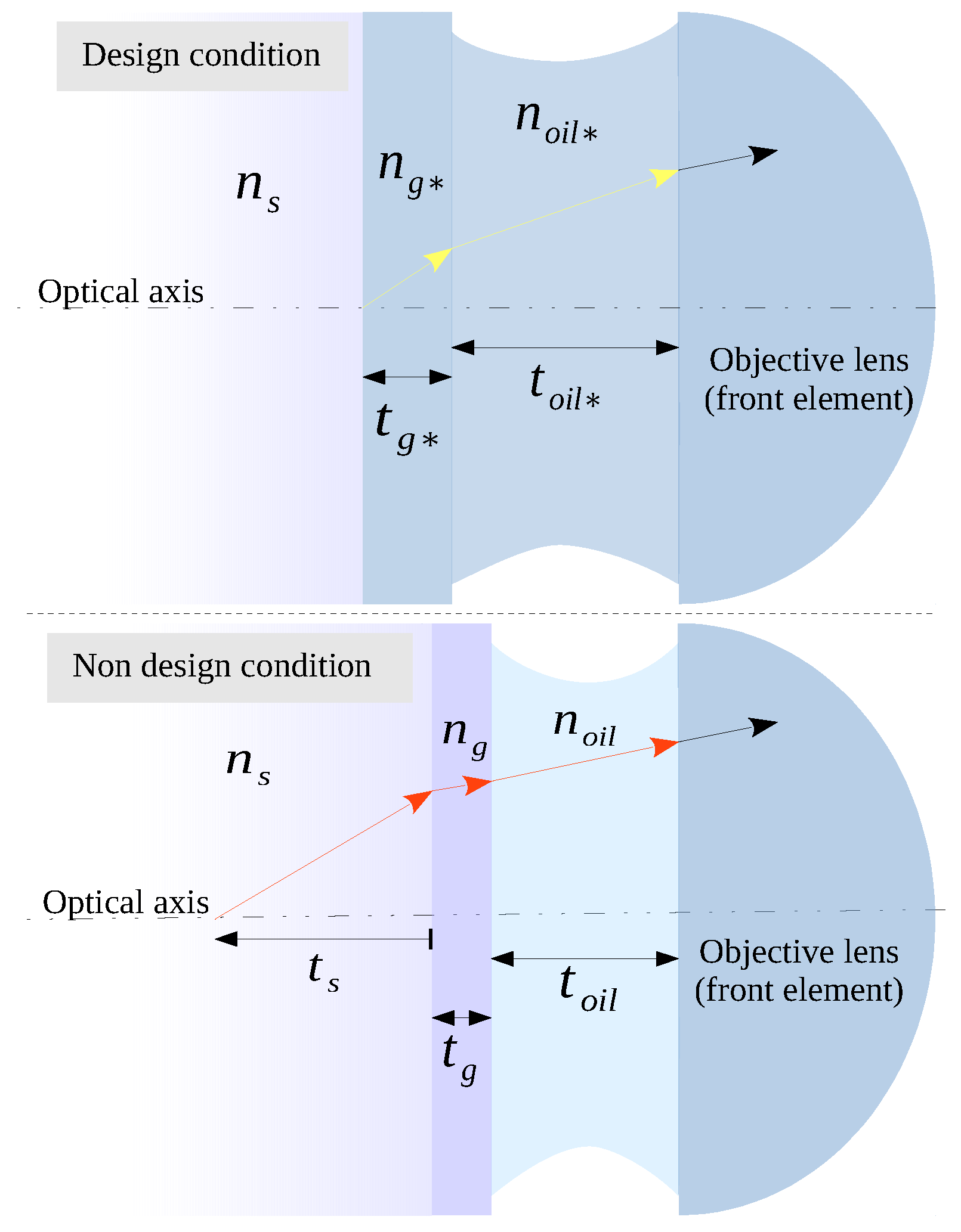
The model developed by Gibson and Lanni [13] provides an accurate way to determine the 3D PSF for a fluorescence microscope. This is based on the calculation of phase aberration (or aberration function) W [1,22,23], from the optical path difference (OPD) between two rays, originating from different conditions. One supposes the optical system used according to optimal settings given by the manufacturer, or design conditions, and the other under non-design conditions, a much more realistic situation. In design conditions (see Figure 1 and

Table 1. Gibson and Lanni model parameters and their descriptions.

Parameter	Description
NA	Numerical aperture
M	Total magnification
$n_{oi{l}^{*}}$	Nominal refractive index of the immersion oil
$t_{oi{l}^{*}}$	Nominal working distance of the lens
$n_{oil}$	Refractive index of the immersion oil used
$n_{g^{*}}$	Nominal refractive index of the coverslip
$t_{g^{*}}$	Nominal thickness of the coverslip
$n_g$	Refractive index of the coverslip used
$t_g$	Thickness of the coverslip used
$n_s$	Refractive index of the medium where the point source is
$t_s$	Point-source position measured from the coverslip’s inner side
$z_{d^{*}}$	Tube length design condition
$z_d$	Tube length in the non-design condition
$x_d,y_d$	Point source planar position measured from the optical axis
$\Delta z$	System defocus

for a reference), the object plane, immediately below the coverslip, is in focus in the design plane of the detector (origin of the yellow arrow). However, in non-design conditions, to observe a point source located at the depth $t_s$ of the specimen, the stage must be moved along the optical axis towards the lens until the desired object is in focus in the plane of the detector (origin red arrow). This displacement produces a decrease in the thickness of the immersion oil layer that separates the front element of the objective lens from the coverslip. However, this shift is not always the same because, if the rays must also pass through no nominal thicknesses and refractive indices, both belonging to the coverslip and the immersion oil, the correct adjustment of the position will depend on the combination of all of these parameters. In any case, in non-design conditions, the diffraction pattern will be degraded from the ideal situation. Indeed, the more apart an acquisition setup is from design conditions, the more degraded the quality of the images will be.

In design conditions, the image of a point source of an ideal objective lens is the diffraction pattern produced by the spherical wave converging to the Gaussian image point in the design plane of the detector that is diffracted by the lens aperture. In this ideal case, the image is considered aberration-free and diffraction-limited. A remarkable characteristic of this model is that the OPD depends on a parameter set easily obtainable from the instrument data sheets. With this initial statement, Gibson and Lanni obtained an approximation to the OPD given by the following expression:

$$\begin{array}{cc}\hfill \mathrm{OPD}\approx & n_{oil}\left[\Delta z+\frac{(z_{d^{*}}-z_d)a^2{n}_{oil}}{z_{d^{*}}{z}_d{\mathrm{NA}}^2}\right]\sqrt{1-{\left(\frac{\mathrm{NA}\rho }{n_{oil}}\right)}^2}+\frac{a^2{\rho }^2(z_{d^{*}}-z_d)}{2n_{oil}{z}_{d^{*}}{z}_d}\hfill \\ & +n_s{t}_s\left\{\sqrt{1-{\left(\frac{\mathrm{NA}\rho }{n_s}\right)}^2}-{\left(\frac{n_{oil}}{n_s}\right)}^2\sqrt{1-{\left(\frac{\mathrm{NA}\rho }{n_{oil}}\right)}^2}\right\}\hfill \\ & +n_g{t}_g\left\{\sqrt{1-{\left(\frac{\mathrm{NA}\rho }{n_g}\right)}^2}-{\left(\frac{n_{oil}}{n_g}\right)}^2\sqrt{1-{\left(\frac{\mathrm{NA}\rho }{n_{oil}}\right)}^2}\right\}\hfill \\ & -n_{g^{*}}{t}_{g^{*}}\left\{\sqrt{1-{\left(\frac{\mathrm{NA}\rho }{n_{g^{*}}}\right)}^2}-{\left(\frac{n_{oil}}{n_{g^{*}}}\right)}^2\sqrt{1-{\left(\frac{\mathrm{NA}\rho }{n_{oil}}\right)}^2}\right\}\hfill \\ & -n_{oi{l}^{*}}{t}_{oi{l}^{*}}\left\{\sqrt{1-{\left(\frac{\mathrm{NA}\rho }{n_{oi{l}^{*}}}\right)}^2}-{\left(\frac{n_{oil}}{n_{oi{l}^{*}}}\right)}^2\sqrt{1-{\left(\frac{\mathrm{NA}\rho }{n_{oil}}\right)}^2}\right\},\hfill \end{array}$$

(1)

whose parameters are described in Table 1. In particular, $\Delta z$ is defined as the best geometrical focus of the system, $a=z_{d^{*}}\mathrm{NA}/{(M^2-{\mathrm{NA}}^2)}^{1/2}$ is the radius of the projection of the limiting aperture and ρ is the normalized radius, these last two being defined in the back focal plane of the objective lens.

With the phase aberration, defined as $W=k\mathrm{OPD}\left(\rho \right)$, where $k=\frac{2\pi }{\lambda }$ is the wave number and λ the wavelength of the source, the intensity field on the detector position ${\mathbf{x}}_d=(x_d,y_d,z_d)$ of the image space ${\mathbb{X}}_{\mathrm{Im}}$ due to a point source placed at the position ${\mathbf{x}}_o=(0,0,t_s)$ of the object space ${\mathbb{X}}_{\mathrm{Ob}}$ of the system in non-design conditions can be computed by Kirchhoff’s diffraction integral:

$$h_{{\mathbf{x}}_d}\left(\mathit{\theta }\right)={\left|\frac{C}{z_d}{\int }_0^1{J}_0\left[ka\rho \frac{\sqrt{x_d^2+y_d^2}}{z_d}\right]e^{jW(\rho ;\mathit{\theta })}\rho d\rho \right|}^2,$$

(2)

being C a constant complex amplitude, $\mathit{\theta }=\{{\theta }_1,{\theta }_2,...,{\theta }_L\}$ the set of the L fixed parameters listed in Table 1 and $J_0$ is the Bessel function of the first kind of first order.

It is of practical interest to relate the detector coordinates ${\mathbf{x}}_d$ in the image space ${\mathbb{X}}_{\mathrm{Im}}$ with the coordinates ${\mathbf{x}}_o=(x_o,y_o,z_o)$ in the object space. This can be done projecting the image plane $(x,y,z_d)$ to the front focal plane. This projection counteracts the magnification and the 180 degree rotation with respect to the optical axis, placing the image on the specimen’s coordinate system [23]. In order to reduce expressions, it will be assumed that $\mathbf{x}$ represents, generically, spatial position.

From a statistic point of view, the Gibson and Lanni model, appropriately normalized, represents the probability distribution of detecting photons in different spatial places. Therefore, without loss of generality, it can be assumed that [24,25]:

$${\int }_{\mathbf{x}\in {\mathbb{X}}_{\mathrm{Im}}}{h}_{\mathbf{x}}\left(\mathit{\theta }\right)d\mathbf{x}=1.$$

(3)

Alternatively, in the discrete formulation, which will be used in this work,

$$\sum _{n=1}^N{h}_n\left(\mathit{\theta }\right)=1,$$

(4)

where N is the total number of voxels and n the voxel position in the object space. Conditional probability is represented by $h_n\left(\mathit{\theta }\right)$ instead of $h\left({\mathbf{x}}_n\right|\mathit{\theta })$, in order to reduce expressions.

2.1. OPD Function Implementation

In the OPD approximation (1), there are terms that cancel if the corresponding nominal and actual parameters are equal. The implementation in GNU Octave [26] coded for this work takes into account all parameters of the given formula. However, it is previously built with the parameters that will be used, evaluating the difference between the corresponding nominal and real parameters and binding those terms to the corresponding parameters whose difference is not zero. This reduces the computational time in those cases where the terms with corresponding parameters are equal.

2.2. Numerical Integration of the Model

The integral of Equation (2) was tested with several numerical integration methods available in GNU Octave [26]. All return similar qualitative results. However, in terms of speed of computation, the Gauss–Kronrod quadrature [27] resolved the integral in a shorter time than the other methods, and, because of this, it was selected to compute the integral of the Equation (2). Since this method could not converge (e.g., by stack overflow of the recursive calls), an alternative method that uses the adaptive Simpson rule is used. The implementation of the Gibson and Lanni model of this work adds a control logic that determines, as a function of the refraction index $n_s$ and the numerical aperture (NA), an upper limit to the normalized radius of integration, ρ. This avoids that expressions within square roots in Equation (1) turn out to be negative.

2.3. Implementation of the 3D PSF Function

A GNU Octave function [26] to generate 3D PSF was implemented. It takes as input the PSF model as an octave handle function, pixel size, plane separation, row number, column number, plane number, normalization type and shift of the PSF peak along the optical axis. The normalization parameter allows two forms of data normalization. The main form for this work corresponds to the total sum of intensities for each plane and relative to the plane with more accumulated intensity. This form simulates the intensity distributions in optical sectioning for a stable source and fixed exposure time. The peak shift parameter allows to center the PSF peak in a specific plane.

2.4. General Model for a Noisy PSF

The digital capture of optical images is a process that can be considered as an additional cause of aberration, due to the incidence of the noise sources involved in the acquisition process ([1], Chapter 12, p. 251). As a general model, it can be considered that the number of photons ${\overline{q}}_n$ in each voxel is given by:

$${\overline{q}}_n\left(\mathit{\theta }\right)=S_{\mathrm{int}}(c\times h_n\left(\mathit{\theta }\right))+S_{\mathrm{ext}},$$

(5)

where $S_{\mathrm{int}}$ represents the intrinsic noise of the signal, c is a constant that converts intensities of $h_n\left(\mathit{\theta }\right)$ to photon flux and $S_{\mathrm{ext}}$ represents extrinsic noise sources of a given signal (e.g., read-out noise); assuming for each noise source a probability distribution model [1,10]. Simulated or acquired data will be called $q_n$.

3. Comparing Experimental and Theoretical 3D PSF

The building of a method for parameter estimation requires the prior definition of a comparison criterion, or objective function, between the parametric model and the data. Then, this function is optimized to find the optimal parameters that, according to the criterion, make the model more similar to the data.

In this report, parameter estimation by least square error, maximum likelihood and Csiszár I-divergence minimization (our own development) are described. These estimation methods lead to non-linear function optimizations, and since the purpose of this study is to compare them, all were approximated to the first order term of their Taylor series representations, obtaining iterative estimators. In other words, assuming that the objective function is given by $\mathrm{OF}\left(\mathit{\theta }\right)$, the problem is to find which θ makes $\mathrm{OF}\left(\mathit{\theta }\right)$ optimum. This is,

$$\frac{\partial \mathrm{OF}\left({\theta }_l\right)}{\partial {\theta }_l}=f\left({\theta }_l\right)\equiv 0.$$

(6)

The basic Taylor series expansion of the non-linear function $f\left({\theta }_l\right)$ is given by,

$$f\left({\theta }_l\right)=f({\theta }_l^{\left(0\right)})+f^{\prime }({\theta }_l^{\left(0\right)})({\theta }_l-{\theta }_l^{\left(0\right)})+\frac{f^{″}({\theta }_l^{\left(0\right)}){({\theta }_l-{\theta }_l^{\left(0\right)})}^2}{2!}+...,$$

(7)

where ${\theta }_l^{\left(0\right)}$ is an arbitrary point near ${\theta }_l$ around which $f\left({\theta }_l\right)$ is evaluated. Therefore, if $\widehat{{\theta }_l}$ is a root of $f\left({\theta }_l\right)$, then the left side of Equation (7) is zero, and the right side of Equation (7) can be truncated to the first order term of the series to get a linear approximation of the root. That is,

$$\widehat{{\theta }_l}\approx {\theta }_l^{\left(1\right)}={\theta }_l^{\left(0\right)}-\frac{f({\theta }_l^{\left(0\right)})}{f^{\prime }({\theta }_l^{\left(0\right)})}.$$

(8)

This approximation can be improved by successive substitutions, obtaining the iterative method known as Newton–Raphson ([28], Chapter 5, pp. 127–129), which can be written as,

$${\theta }_l^{(m+1)}={\theta }_l^{\left(m\right)}-\frac{f({\theta }_l^{\left(m\right)})}{f^{\prime }({\theta }_l^{\left(m\right)})},$$

(9)

where the superscript $\left(m\right)$ indicates the iteration number. The initial estimate (i.e., $m=0$) has to be near the root to ensure the convergence of the method.

3.1. Least Square Error

Historically, in the signal processing field, the square error (SE) has been used as a quantitative metric of performance. From an optimization point of view, SE exhibits convexity, symmetry and differentiability properties, and its solutions usually have analytic closed forms; when not, there exist numerical solutions that are easy to formulate [29]. Kirshner et al. [12] developed and evaluated a fitting method based on the SE optimization between data and the Gibson and Lanni model [13]. They used the Levenberg–Marquardt algorithm to solve the non-linear least square problem, obtaining low computation times, as well as accurate and precise approximation to the point source localization. In the present work, this algorithm was not considered. Instead, an iterative formulation for the estimator was obtained, considering the SE objective function given by:

$$\mathrm{SE}\left(\mathit{\theta }\right)=\sum _{n=1}^N{(q_n-{\overline{q}}_n\left(\mathit{\theta }\right))}^2.$$

(10)

Following the procedure given by Equations (6)–(9), the minimum of SE$\left(\mathit{\theta }\right)$ is found making its partial derivatives equal to zero, that is:

$$\frac{\partial \mathrm{SE}\left({\theta }_l\right)}{\partial {\theta }_l}=\sum _{n=1}^N\left(q_n-{\overline{q}}_n\left({\theta }_l\right)\right)\frac{\partial {\overline{q}}_n\left({\theta }_l\right)}{\partial {\theta }_l}\equiv 0.$$

(11)

The representation of Equation (11) to the first order term of the Taylor series leads to the following iterative formulation of the estimator:

$${\theta }_l^{(m+1)}={\theta }_l^{\left(m\right)}-\frac{{\sum }_{n=1}^N(q_n-{\overline{q}}_n({\theta }_l^{\left(m\right)}))\frac{\partial {\overline{q}}_n({\theta }_l^{\left(m\right)})}{\partial {\theta }_l^{\left(m\right)}}}{{\sum }_{n=1}^N\left(\frac{{\partial }^2{\overline{q}}_n({\theta }_l^{\left(m\right)})}{{\partial {\theta }_l^{\left(m\right)}}^2}(q_n-{\overline{q}}_n({\theta }_l^{\left(m\right)}))-{\left(\frac{\partial {\overline{q}}_n({\theta }_l^{\left(m\right)})}{\partial {\theta }_l^{\left(m\right)}}\right)}^2\right)}.$$

(12)

3.2. Csiszár I-Divergence Minimization

It has been argued that in cases where data do not belong to the set of positive real numbers, the SE does not reach a minimum [30,31], this being a fact in optical images, because the intensities captured are always nonnegative. An alternative is to use Csiszár I-divergence, which is a generalization of the Kullback–Leibler information measure between two probability mass functions (or density, in the continuous case) p and r. It is defined as [30]:

$$I\left(p\right|\left|r\right)=\sum _{n=1}^N{p}_n\log \left(\frac{p_n}{r_n}\right)-\sum _{n=1}^N\left(p_n-r_n\right).$$

(13)

Compared with the Kullback–Leibler information measure, Csiszár adjusts the p and r functions for those cases in which their integrals are not equal [31], adding the last summation term on the right side of the Equation (13). Because of this, $I\left(p\right|\left|r\right)$ has the following properties:

• $I\left(p\right|\left|r\right)\ge 0$
• $I\left(p\right|\left|r\right)=0$ when $p=r$

Consequently, for a fixed r, $I\left(p\right|\left|r\right)$ has a unique minimum, which is reached when $p=r$. The probability mass function r operates as a reference from which the function p follows peaks and valleys of r. In this work, it is proposed that the reference function will be the data normalized so that their sum is equal to one. This normalized data form, which will be called $d_n$, represents the relative frequency of the photon count in each spatial position. This is,

$$d_n=\frac{q_n}{{\sum }_{n=1}^N{q}_n}.$$

(14)

Then, replacing $p_n$ in Equation (13) by $h_n\left(\mathit{\theta }\right)$ and $r_n$ by $d_n$, the I-divergence between the normalized data and the theoretical distribution $h_n\left(\mathit{\theta }\right)$ is given by:

$$I\left(h\left(\mathit{\theta }\right)\right|\left|d\right)=\sum _{n=1}^N{h}_n\left(\mathit{\theta }\right)\log \frac{h_n\left(\mathit{\theta }\right)}{d_n}-\sum _{n=1}^N\left(h_n\left(\mathit{\theta }\right)-d_n\right).$$

(15)

To minimize $I\left(h\right(\mathit{\theta }\left)\right|\left|d\right)$, its partial derivatives must be equal to zero, that is:

$$\frac{\partial I\left(h\left({\theta }_l\right)\right|\left|d\right)}{\partial {\theta }_l}=\sum _{n=1}^N\frac{\partial h_n\left({\theta }_l\right)}{\partial {\theta }_l}\log \left(\frac{h_n\left({\theta }_l\right)}{d_n}\right)\equiv 0.$$

(16)

Representing Equation (16) in Taylor series and approximating to the term of first order, the following iterative estimator is obtained:

$${\theta }_l^{(m+1)}={\theta }_l^{\left(m\right)}-\frac{{\sum }_{n=1}^N\frac{\partial h_n({\theta }_l^{\left(m\right)})}{\partial {\theta }_l^{\left(m\right)}}\log \left(\frac{h_n({\theta }_l^{\left(m\right)})}{d_n}\right)}{{\sum }_{n=1}^N\left(\frac{{\partial }^2{h}_n({\theta }_l^{\left(m\right)})}{{\partial {\theta }_l^{\left(m\right)}}^2}\log \left(\frac{h_n({\theta }_l^{\left(m\right)})}{d_n}\right)+h_n^{-1}({\theta }_l^{\left(m\right)}){\left(\frac{\partial h_n({\theta }_l^{\left(m\right)})}{\partial {\theta }_l^{\left(m\right)}}\right)}^2\right)}.$$

(17)

3.3. Maximum Likelihood

The maximum likelihood principle establishes that data that occur must have, presumably, the maximum probability of occurrence [25]. Aguet et al. [10] used this idea to build an estimation method of the position of a point source along the optical axis. The likelihood function (or log-likelihood), represented by the expected number of photons in a point of the space, is given by:

$$\log L(q_n,\mathit{\theta })=\sum _{n=1}^N{q}_n\log {\overline{q}}_n(\mathit{\theta })-{\overline{q}}_n\left(\mathit{\theta }\right)-\log (q_n!),$$

(18)

which is built under the assumptions of a forward model given by Equation (5), with $S_{\mathrm{int}}$ following a Poisson distribution and $S_{\mathrm{ext}}$ representing read-out noise of the acquisition device, ${\sigma }_{ro}$, which follows a Gaussian distribution. With these assumptions, the authors build an iterative formulation of the estimator based on the maximization for the log-likelihood function between captured data and the Gibson and Lanni model. They also used a numerical approximation to the term of the first order of the Taylor series, obtaining:

$${\theta }_l^{(m+1)}={\theta }_l^{\left(m\right)}-\frac{{\sum }_{n=1}^N\frac{\partial {\overline{q}}_n({\theta }_l^{\left(m\right)})}{\partial {\theta }_l^{\left(m\right)}}\left(\frac{q_n}{{\overline{q}}_n({\theta }_l^{\left(m\right)})}-1\right)}{{\sum }_{n=1}^N\left(\frac{{\partial }^2{\overline{q}}_n({\theta }_l^{\left(m\right)})}{{\partial {\theta }_l^{\left(m\right)}}^2}\left(\frac{q_n}{{\overline{q}}_n({\theta }_l^{\left(m\right)})}-1\right)-{\left(\frac{\partial {\overline{q}}_n({\theta }_l^{\left(m\right)})}{\partial {\theta }_l^{\left(m\right)}}\right)}^2\frac{q_n}{{\left({\overline{q}}_n({\theta }_l^{\left(m\right)})\right)}^2}\right)}.$$

(19)

3.4. Implementation of the Estimation Methods

The above described estimation methods were implemented as GNU Octave functions [26], taking as input values the experimental PSF data properly normalized, a function handle to compute theoretical PSF and, as output conditions, an absolute tolerance value and a maximum number of iterations in case the methods do not converge. The derivatives of the Gibson and Lanni model in the iterative Equations (12), (17) and (19) were evaluated numerically with a forward step. The outputs of these Octave functions return the estimation for each iteration.

3.5. Lower Bound of the Estimation Error

Independently of the estimation method used to fit the parameters of a model, if the estimator is unbiased, its variance is bounded. This lower bound to the estimation method precision is commonly known as the Cramer–Rao bound. It is a general result that depends only on the image formation model ([25], Chapter 17, pp. 391–392). Aguet et al. [10] obtained a form for the Cramer–Rao bound calculation for axial localization, which is based on the image formation model given by Equation (5) with intrinsic and extrinsic noise sources that are Poisson distributed. Abraham et al. [15] used two forms of this bound for planar localization: a fundamental (or theoretical) one, which considers ideal detection conditions, and a practical bound, which ponders the limitations of the detector and noise sources that corrupt the signal. In the current work, the form obtained by Aguet et al. [10] was used.

4. Results

4.1. Tests on Simulated Data

All tests were performed regarding the estimation of the parameter ${\theta }_l:=t_s$ (see Table 1). The estimator ${\theta }_l^{\left(m\right)}$ obtained by any of the forms given by the iterative Equations (12), (17) and (19) is represented by $t_s^{\left(m\right)}$ to indicate iterations, or alternatively by ${\widehat{t}}_s$. Three conditions of noisy data in several intensity levels of the photon signal were analyzed. These are classified as Noise Case I (NCI), which represents a unique intrinsic noise source, which follows a Poisson distribution. Noise Case II (NCII) is a situation that presents the NCI and an extrinsic source of noise that follows a Gaussian distribution with known mean (2500) and variance (25). Noise Case III (NCIII) is a condition where the NCI is present and there is an additive extrinsic noise source that follows a Poisson distribution with known mean set up to 25 photons. The signal intensity expected at the focal plane ranged between $2^8$ and $2^{16}$ photon counts. For reference, with these levels of photon counts and noise conditions, the signal-to-noise ratio ranges from 11–24 dB.

4.1.1. Cramer–Rao Lower Bound Analysis

A first analysis of the CRB behavior to changes on acquisition parameters was made with the general purpose of finding out whether the application of estimation techniques makes sense in some real acquisition configurations. The selected parameters for analysis were pixel size, pixel number, acquired photons at a plane and background level. As mentioned previously, the CRB bound was computed by the formulation obtained by Aguet et al. [10] that has the form:

$$\mathrm{Var}\left({\theta }_l\right)\ge {\displaystyle \frac{1}{{\sum }_{n=1}^N{\overline{q}}_n{\left({\theta }_l\right)}^{-1}{\left(\frac{\partial {\overline{q}}_n\left({\theta }_l\right)}{\partial {\theta }_l}\right)}^2}},$$

(20)

where $\mathrm{Var}\left({\theta }_l\right)$ represents the variance of the estimator ${\theta }_l$ and $\frac{\partial {\overline{q}}_n\left({\theta }_l\right)}{\partial {\theta }_l}$ was evaluated using a finite difference.

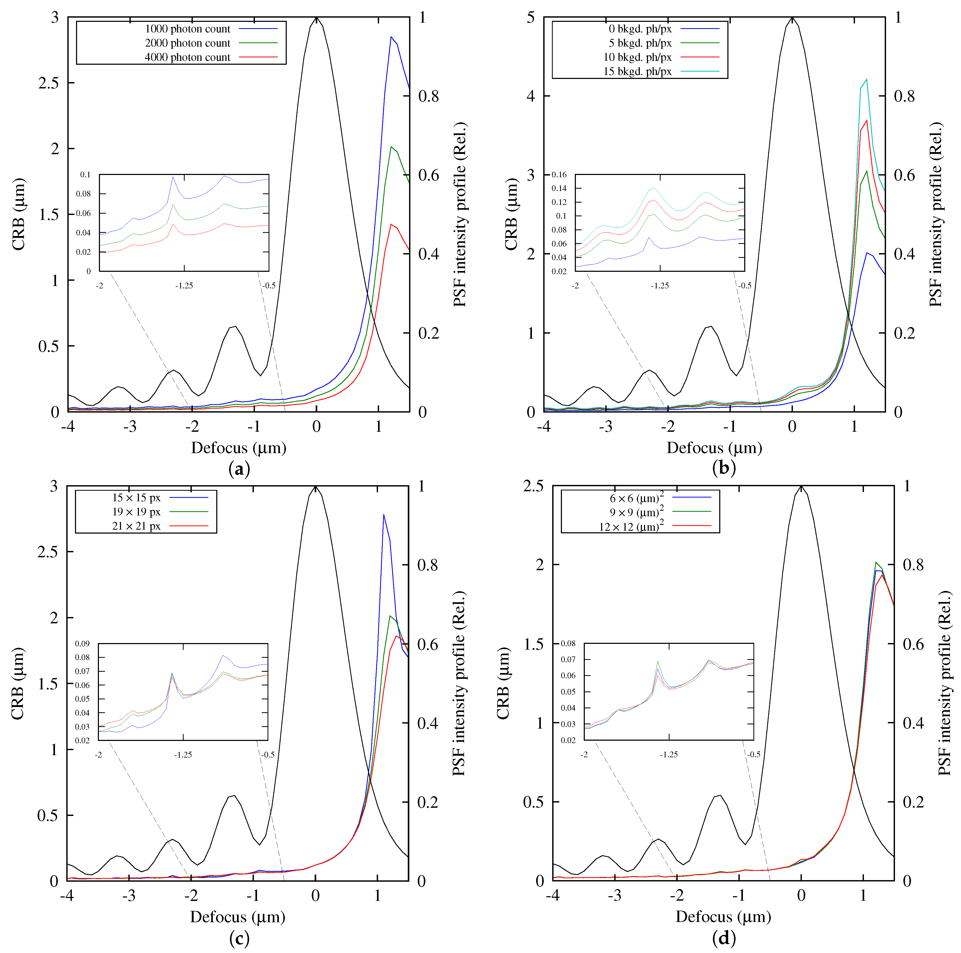
The CRB was computed for each plane along the optical axis for $t_s=5\mathsf{\mu }$m and then plotted as a defocus function, not the system defocus ($\Delta Z$) of Equation (1), but the plane position as a function of the PSF peak (see Figure 2). In general, it is noted that CRB shows an important change in relation to the position of the PSF peak. Those defocused planes between the lens and the PSF peak, or negative defocus (−DF), generate a CRB significantly smaller than those that are beyond the PSF peak, or positive defocus (+DF). Additionally, the CRB becomes smaller as −DF increases in magnitude (see Figure 2a). However, it must be clarified that the CRB computed for each plane has the same photon count, which is something that does not happen in practice because exposition time is generally fixed during optical sectioning acquisition.

Figure 2a shows, as expected, that increasing the photon count decreases the CRB. Conversely, an increase of the background level worsens the achievable precision (see Figure 2b). The estimation error, for large defocus, becomes smaller if a greater number of pixels is used. This is because more pixels are needed to cover the wide spreading that the PSF has at large defocus situations. Finally, no significant changes of the CRB versus pixel size can be observed for the values tested (Figure 2d).

4.1.2. Convergence Test

The convergence of methods was evaluated with free-noise data and by using an approximation of the rate of convergence (ROC) given by:

$${\alpha }_{\mathrm{ROC}}\approx \frac{\log (e^{(m+1)}/e^{\left(m\right)})}{\log (e^{\left(m\right)}/e^{(m-1)})},$$

(21)

where $e^{\left(m\right)}=t_s^{\left(m\right)}-t_s^{(m-1)}$.

Results showed that all methods generate a sequence of linear logarithmic estimations with a similar final number of iterations (see

Table 2. Convergence test. ROC, rate of convergence; MIDIV, I-divergence minimization; LSQR, non-linear least square.

Method	Iterations	${\mathit{\alpha }}_{\mathbf{ROC}}$
MIDIV	9	1.0
ML	9	1.0
LSQR	10	1.0

).

4.1.3. Exploratory Testing

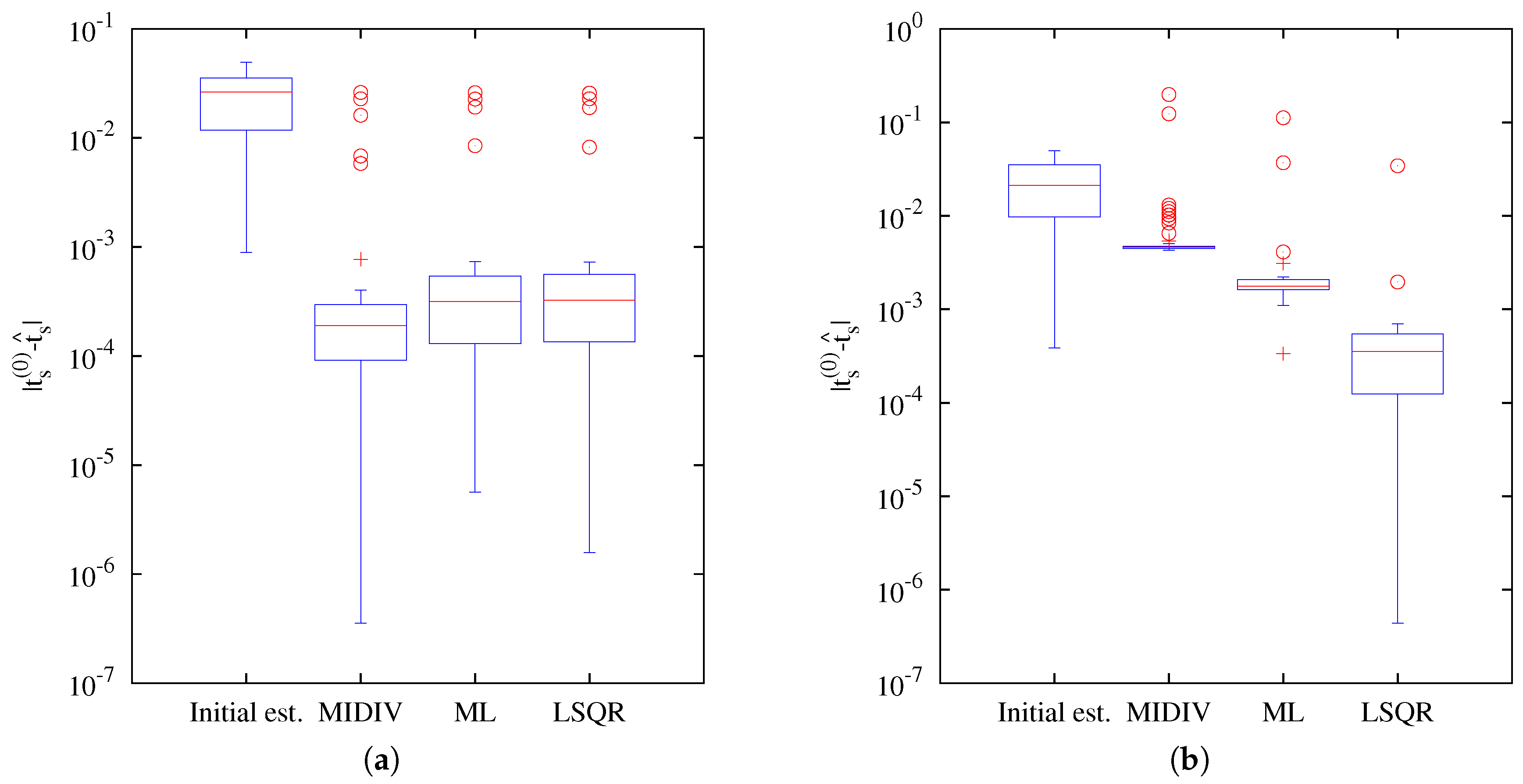
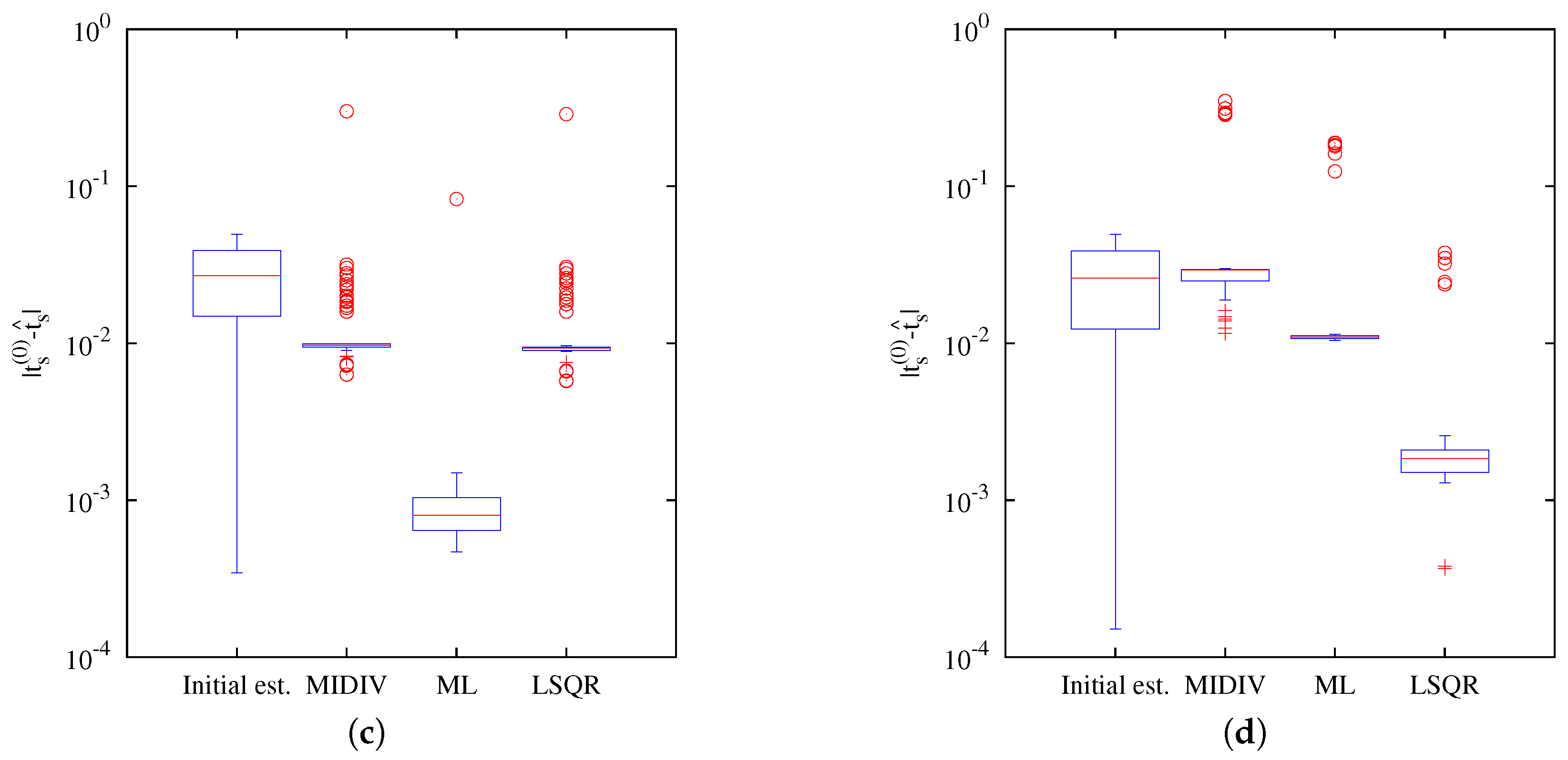
Before the extensive testing of methods, an exploratory analysis was made with the aim of knowing how estimations of the methods are distributed regarding the initial estimate. It also allowed defining the range of the initial estimates that yield an acceptable convergence. Thus, to carry out this test, several initial estimates were generated from a uniform distribution in a small interval that encloses the actual value, or ground truth, $t_s=5$ ($\mathsf{\mu }$m). For each run, the methods used the same initial estimates of the mentioned randomization, the maximum number of iterations and relative tolerance. The results of free-noise data, resumed on the boxplot of Figure 3a, showed that the methods improved precision, that is, the distribution of the estimation residuals becomes narrower than the residuals of initial estimates. However, this is not the case for noisy data, because estimations obtained by methods change for each PSF realization. Figure 3b–d shows how precision is degraded under the presence of noisy data. For this reason, an extensive test with several PSF realizations was carried out to find out how the estimation of the methods performs on noisy data.

4.1.4. Extensive Testing of Methods

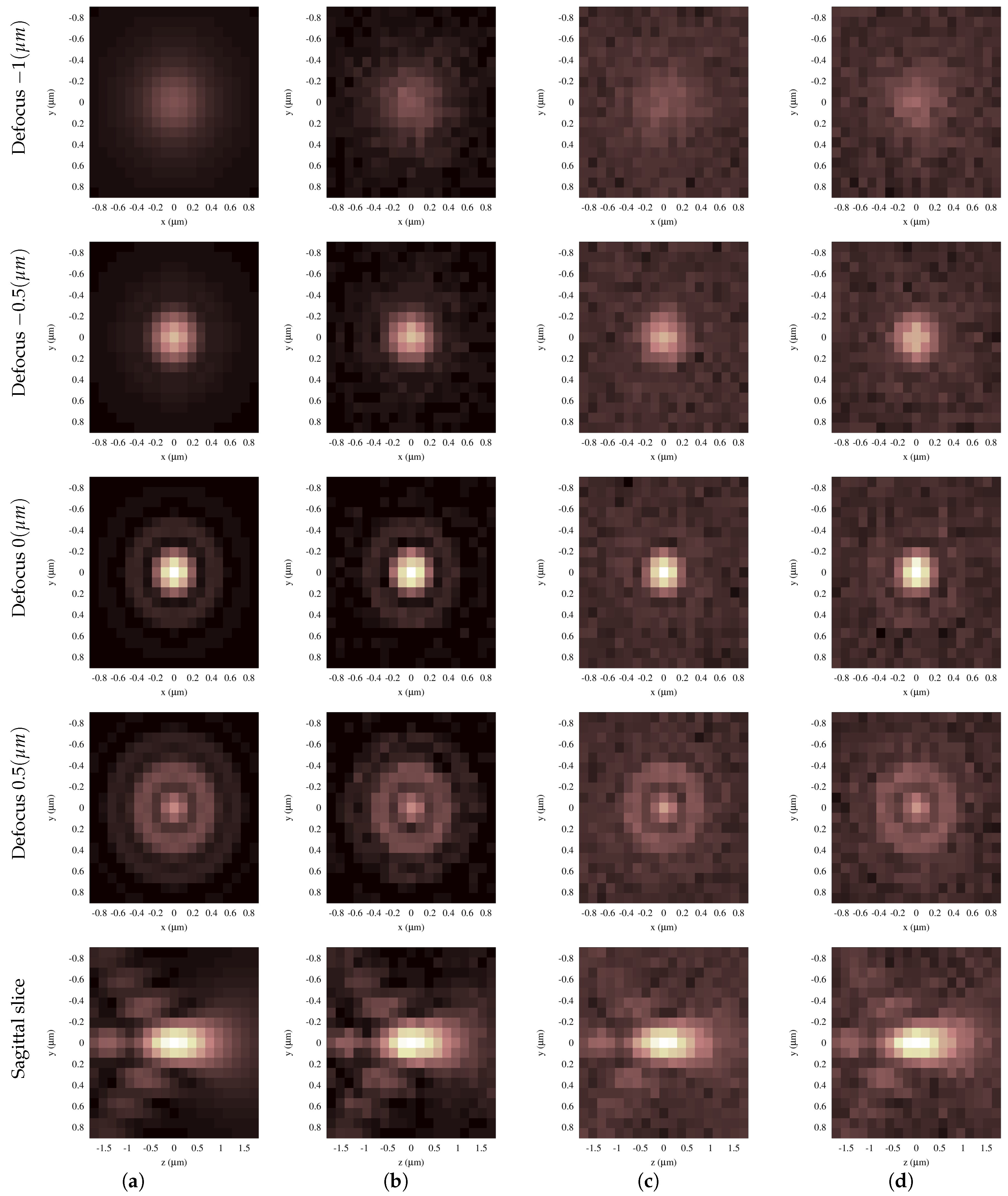
Based on the previous CRB analysis and exploratory testing, as well as the features of the instrumental available, simulated images were generated considering an emission wavelength of 560 nm, NA $1.35$, magnification $100\times$, working distance 100 $\mathsf{\mu }$m, pixel size 9 × 9 $\mathsf{\mu }$m${}^2$ in the image space, $19\times 19$ pixels and an offset level of 2500. Methods were also tested with a sagittal slice with the PSF peak centered and 19 planes. Figure 4 depicts some sample images as used for analysis.

Methods were compared analyzing their results from a set of 3000 PSF realizations for each noise condition generated at $t_s=5$ $\mathsf{\mu }$m. Initial estimates were randomly generated from a uniform distribution in the range of 5.000 ± 0.500 $\mathsf{\mu }$m for optical sections and in the range of 5.000 ± 0.25 $\mathsf{\mu }$m for the sagittal slice. As a general comparison criterion, confidence intervals (CI) of the statistics were computed with a $0.1\%$ confidence level by the nonparametric bootstrap technique based on percentiles ([32], Chapter 8, p. 277 and [33], Chapter 13).

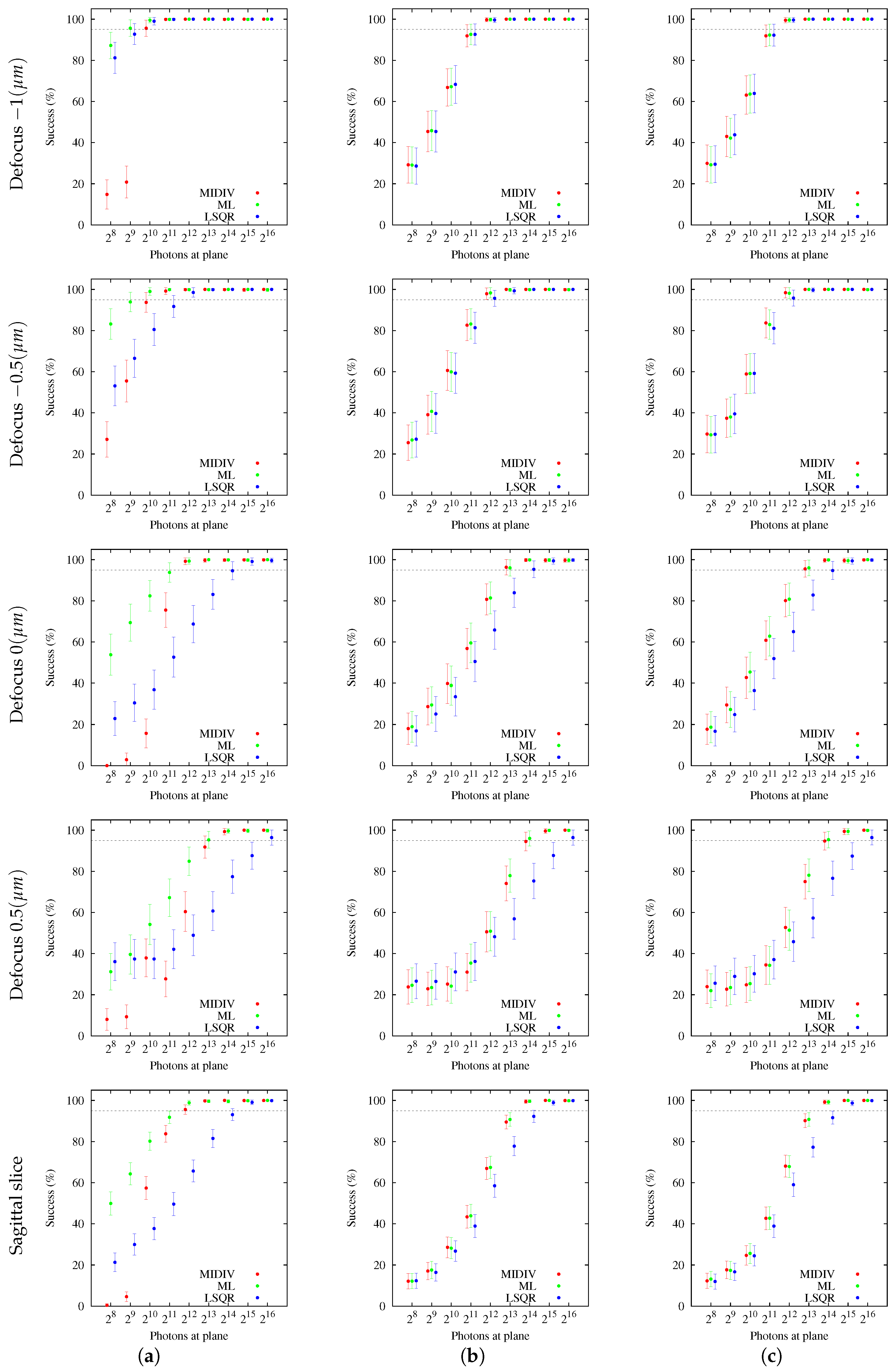
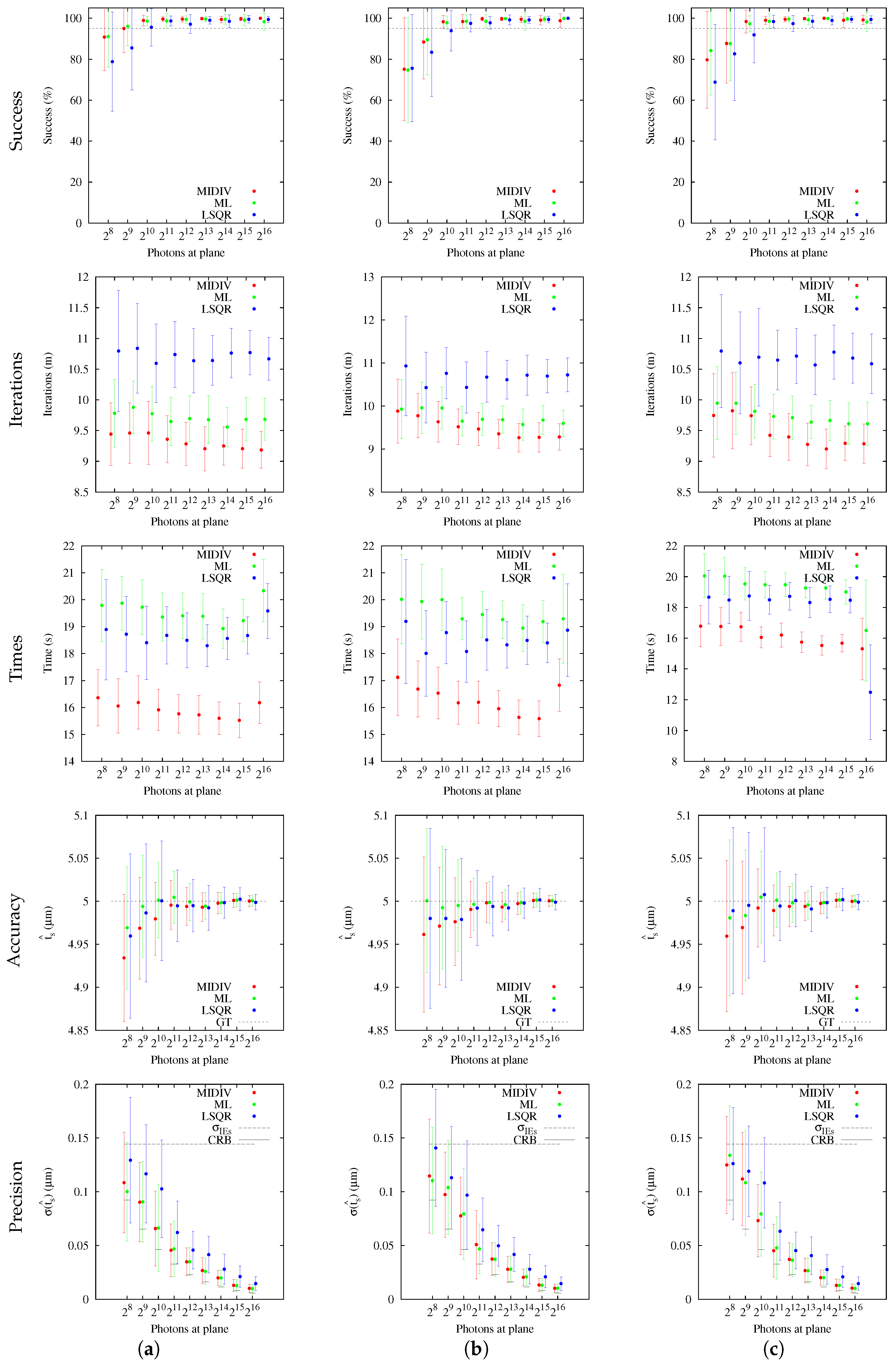
The first criterion used for analyzing and comparing the estimations of the methods was the success percentage. This was computed considering those estimations that did not overtake the maximum number of iterations or that fell in the interval of initial estimates. A $95\%$ success was adopted as a criterion for the comparative analysis (dashed line at $95\%$ for all subfigures in Figure 5). According to this, estimation results in all analyzed directions show that methods are more successful when the most −DF optical sections are used. For all optical sections and sagittal slices, when an extrinsic noise source (NCII or NCIII) is added, the success percentage of the methods is worsened. However, no significant difference was found between noise sources (compare the same method in Figure 5a,b). On the contrary, some dissimilar behaviors were found between methods. For NCI, ML was shown to be more successful than MIDIV and LSQR for almost all optical sections and the sagittal slice. For NCII and NCIII, ML and MIDIV showed the same behavior, achieving a better success percentage than LSQR for the same photon count. Once the success percentage was computed, the other measurements—times, iterations, mean and standard deviations—were computed using only those estimations that converged successfully.

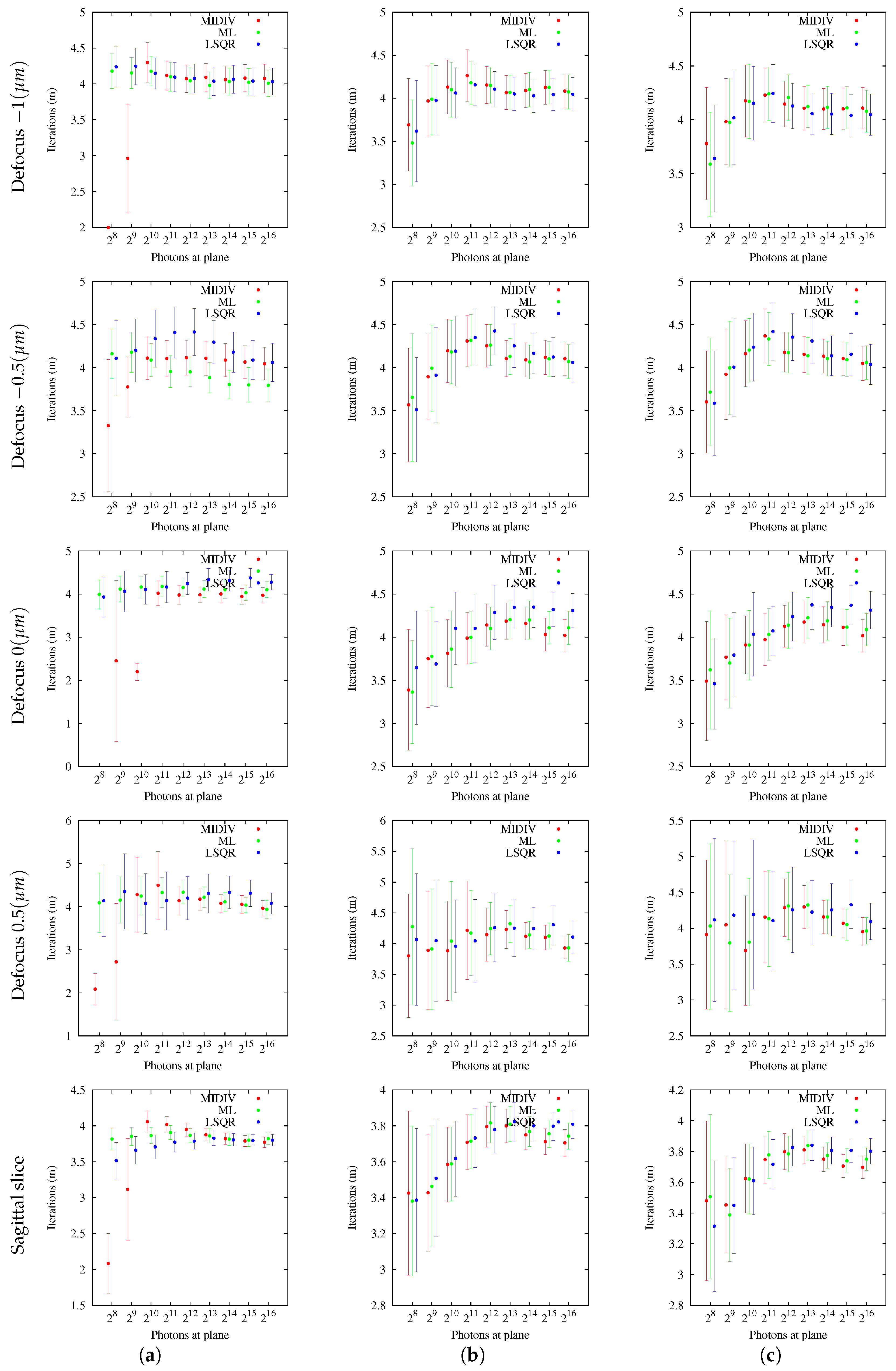
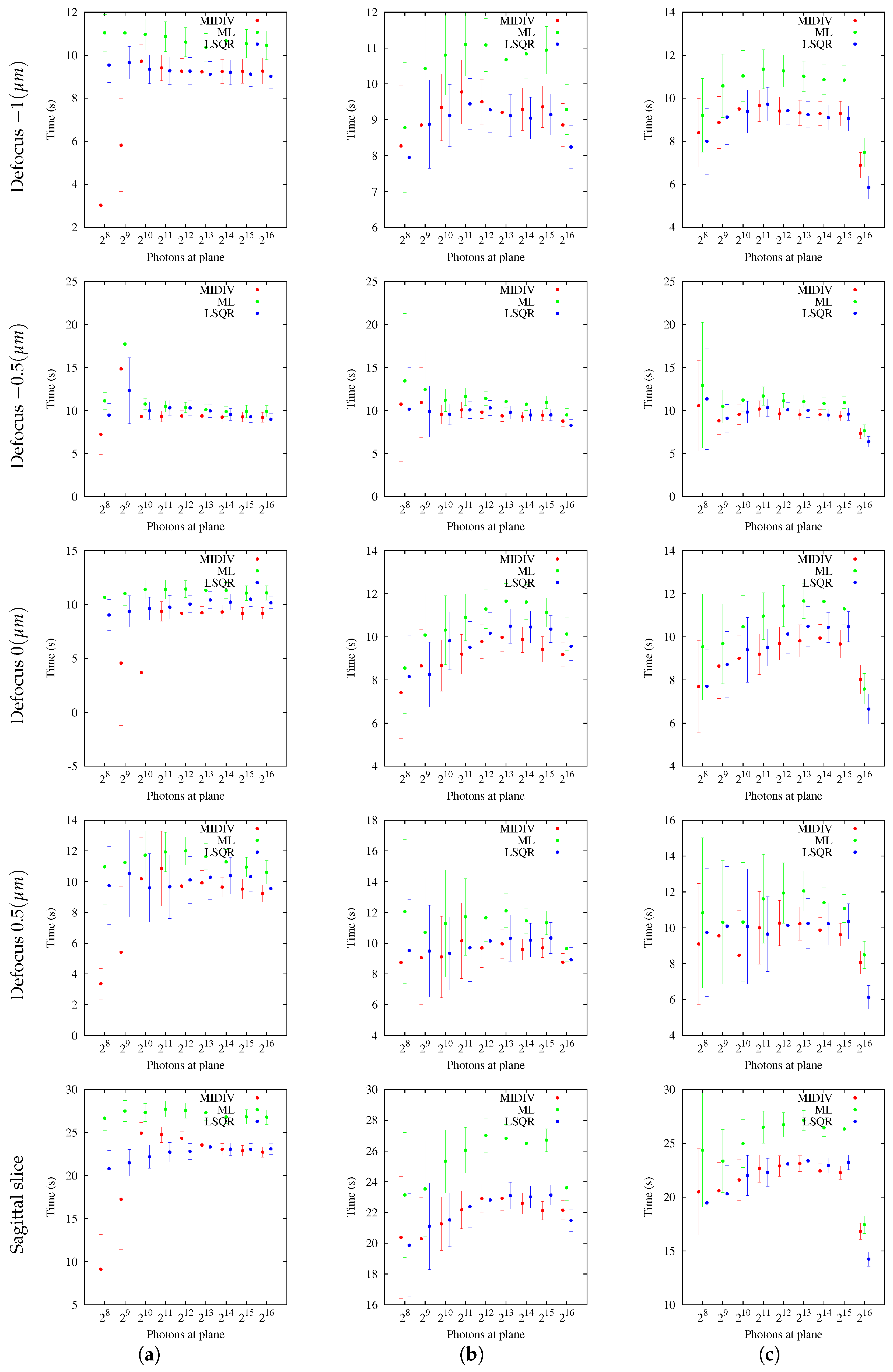
The number of iterations that methods performed (summarized in Figure 6) was practically the same (four iterations) for all directions analyzed and all noise conditions. In general, no differences were found in the number of iterations between methods. The mean number of iterations did not change with the photon count. Regarding estimation times, as can be seen in Figure 7, ML appeared to be slower than LSQR and MIDIV in the most −DF optical sections and sagittal slices. In the remaining cases, methods needed the same computing time.

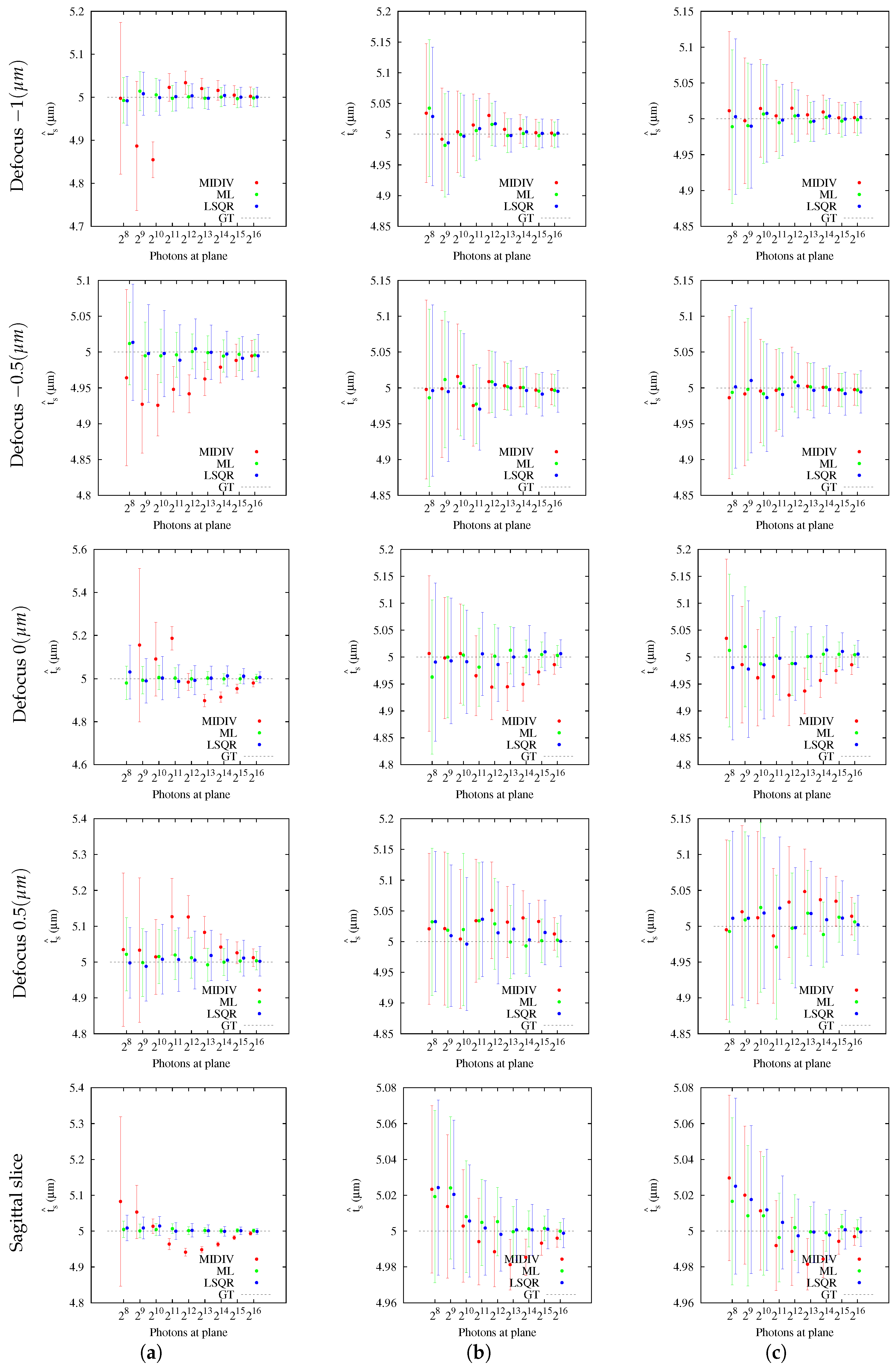
The accuracy and precision of each method were measured using the means and standard deviations of the estimations [3], respectively. The standard deviations were also compared with the CRB to find out if the studied methods achieve this theoretical bound and, in the case of an affirmative answer to this question, to analyze under which conditions. Results, summarized in Figure 8, showed that the CIs for the estimation means returned by the three methods contained the ground truth in most cases, but especially MIDIV showed statistically-significant differences in some photon count levels in both analysis directions for optical sections and sagittal slices, exhibiting a less accurate behavior than the other ones. It can be also noted that the mean estimations of the three methods tend asymptotically towards the ground truth, as the photon count increases. Additionally, the CIs of the mean estimations are narrower in most −DF planes compared with in focus and +DF sections. For the same defocus, when an additive noise source is present (NCII or NCIII), the mean’ CIs become larger, but there are no differences between methods nor between noise sources.

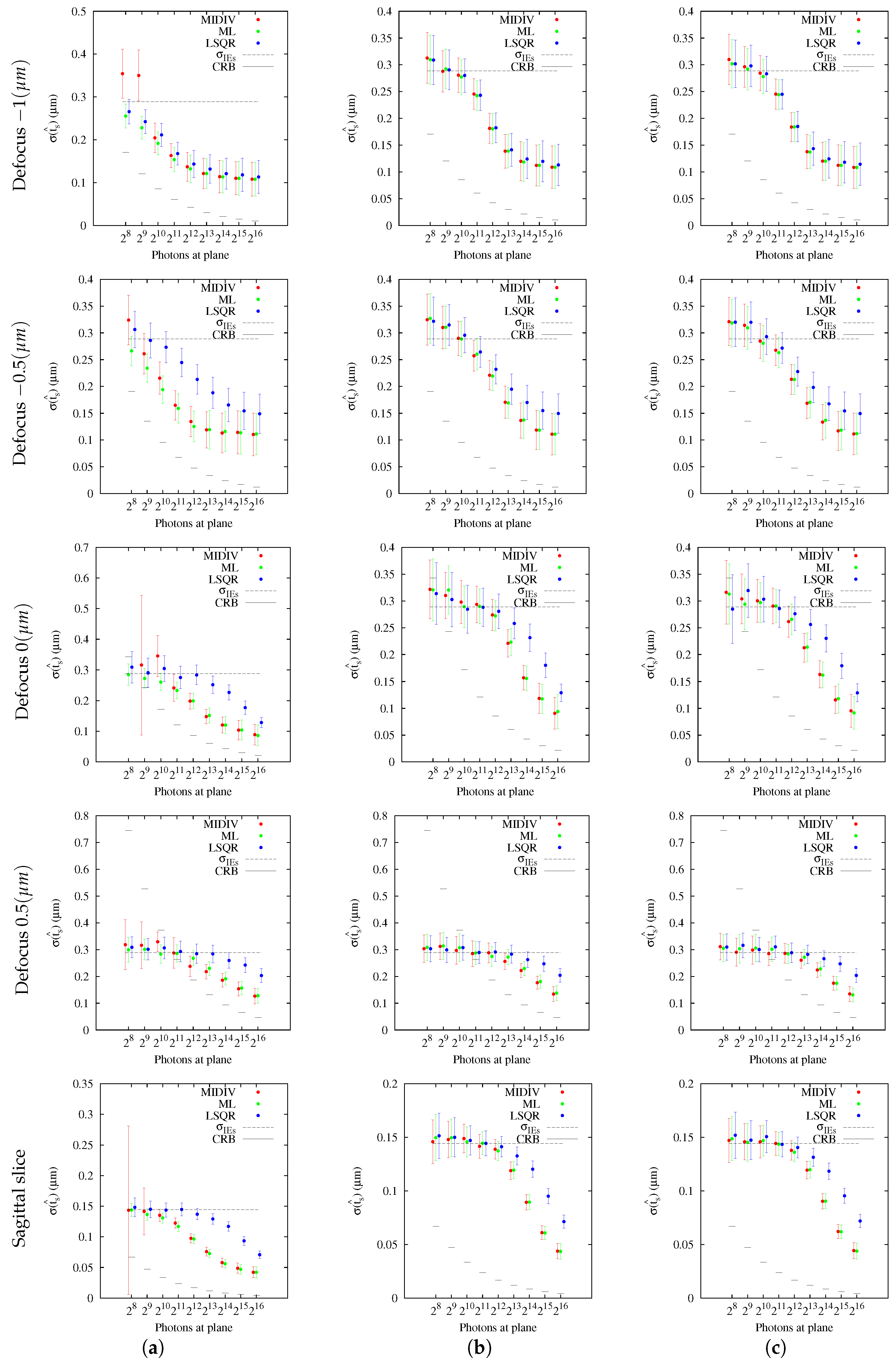
Results related to precision are summarized in Figure 9. It can be observed that the precision of the three methods is practically the same when using optical sections with large −DF for all noise cases. LSQR was shown to be statistically less precise than ML and MIDIV for NCI when −DF or +DF optical sections close to the PSF peak were used. For NCII and NCIII, all methods achieved the same precision, which was better with most −DF optical sections. For optical sections placed at Defocus 0 and 0.5 ($\mathsf{\mu }$m), for low SNR, they seem to achieve precision beyond the theoretical bound, but this should be taken carefully because, in these cases, the CRB is much larger than the standard deviation of the initial estimates (≈0.28 $\mathsf{\mu }$m). For instance, for the optical section placed at −0.5 ($\mathsf{\mu }$m), the worst CRB is around 200 (nm). On the contrary, the CRB of the optical section at 0.5 ($\mathsf{\mu }$m) is around 750 (nm). For all directions analyzed, as photon count increases, the CRB decreases. Similar results were obtained for the NCII and NCIII. However, methods require, as expected, more photons to achieve a precision better than the initial estimates. There are no differences between these noise cases; in fact, the results are practically the same. When estimation methods were applied to a sagittal slice, MIDIV and ML did not exhibit significant differences in precision, but they did with LSQR. All methods improved the precision as the photon count increases. The precision achieved by methods is better than the one obtained with optical sections using the same tolerance. However, it must be mentioned that the range of the initial estimates had to be narrowed to make the pool of estimations statistically manageable. This is because when the same range of optical sections was used, a very low success percentage was obtained.

Previous analysis showed that, in precision terms, all methods would estimate better if a sagittal slice were used. This suggests that there is more information of the parameter $t_s$ in the optical axis direction. However, in a general evaluation, no method seems to be more successful and accurate using a sagittal slice. This suggested an additional test with only the optical axis data. In this test, a larger number of photons was considered with the purpose of evidencing whether methods’ precision will achieve the CRB. Results, summarized in Figure 10, showed that methods have a similar behavior when the data of the optical axis are considered. For the signal levels considered, all methods were successful in estimation, MIDIV being qualitatively faster than ML and LSQR. In these conditions, the means’ CIs of the three methods’ estimation include the ground truth, and as the photon count increases, CIs become narrower. In relation to precision, except for low SNR where standard deviations’ CIs are very large, only ML and MIDIV achieved the CRB, while LSQR did not.

4.2. Axial Position Estimation of an Experimental PSF

The setup proposed by Aguet et al. [10,34] was followed. Briefly, a 0.170 ± 0.005 $\mathsf{\mu }$m diameter fluorescent nanobead stock solution ($3\times {10}^9$ beads/mL) was diluted to 1:100 in distilled water following the supplier’s instructions (PS-Speck Microscope Point Source Kit; Thermo Fisher Scientific Inc., Eugene, OR, USA). Drops of the solution were placed and gently extended over both the slide and cover slip and then dried in darkness. The glass faces were subsequently put together with a small drop of anti-fading mounting medium between them, allowing a thin layer to form. Glasses were sealed using colorless nail polish to avoid displacements. The image acquisition was carried out with an Olympus BX50 microscope, modified for optical sectioning [35,36]. Optical sections were taken every 180 nm. Images were saved in 16-bit TIFF file format.

The axial position $t_s$ of the experimental PSF was estimated by the three ways outlined in this work. The data used were the optical sections of the nanobeads that remained attached to the slide. As a first approximation, a forward computation of the I-divergence Equation (15), log-likelihood Equation (18) and square error Equation (10) functions was carried out starting from the interval between 65 and 90 $\mathsf{\mu }$m of depth. Results were graphically analyzed to delimit a smaller interval that contained the optimum to run the estimation methods. Once the position was estimated by the three methods, and since it is not possible to know the actual position of the point source, the FWHM, in both the capture plane and optical axis, were evaluated as alternative comparison criteria.

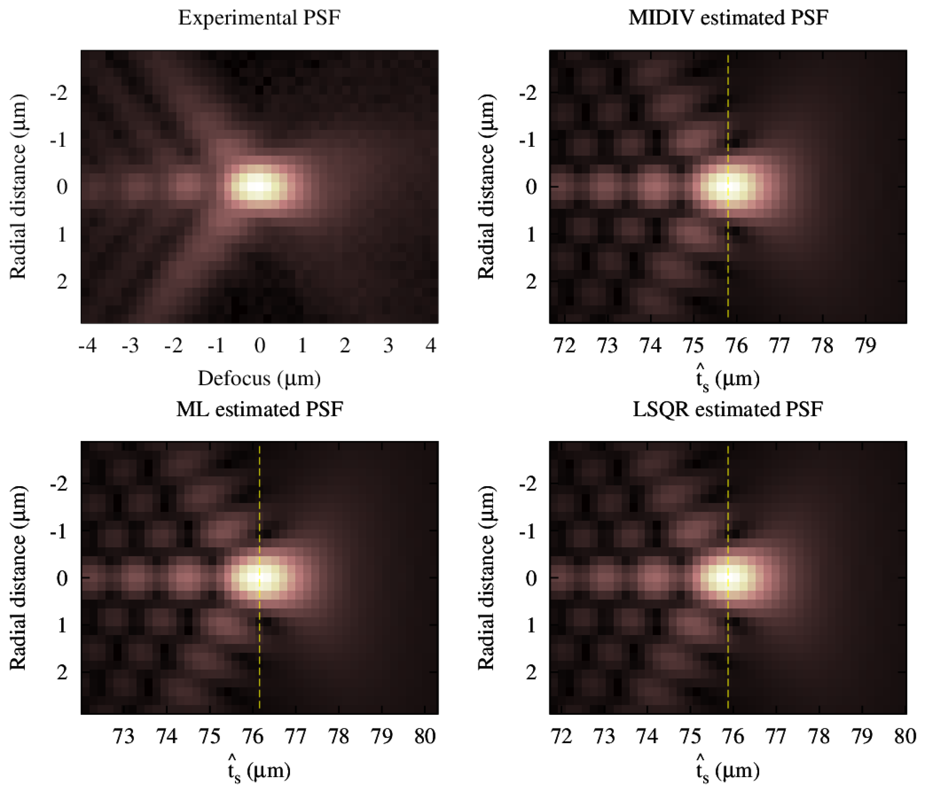
The estimation methods gave qualitatively similar results as can be observed in Figure 11. According to the FWHM comparison, all methods yielded the same result up to the third decimal, as can be observed from

Table 3. FWHM measurements on experimental PSF and the Gibson and Lanni model after estimating $t_s$ with the MIDIV, ML and LSQR methods.

	Axial ($\mathsf{\mu }$m)	Lateral ($\mathsf{\mu }$m)
Exp. PSF	1.303	0.377
MIDIV	1.301	0.387
ML	1.301	0.387
LSQR	1.301	0.387

.

5. Discussion

To our knowledge, just a few ways of parameter estimation methods for theoretical PSF have been developed, and there are no comparative studies of parameter estimation methods applied to microscopy PSF theoretical models. The aim of this work was to contribute to these particular aspects, by carrying out a comparative computational study of three parameter estimation methods for the theoretical model of Gibson and Lanni PSF [13]. This was applied to the position estimation of a point source along the optical axis. The parameter estimation methods analyzed were: Csiszár I-divergence minimization (a previously unpublished own method), maximum likelihood [10] and least square [12]. Since all expressions to optimize are of a non-linear nature, they were approximated using the same numerical representation, obtaining three iterative algorithms that differ in the comparison criteria between the data and model. As an application, the position on the optical axis of an experimental 3D PSF is estimated by the three methods, taking the difference of the FWHM between the estimated and experimental 3D PSF as a comparison criterion.

5.1. Gibson and Lanni Model

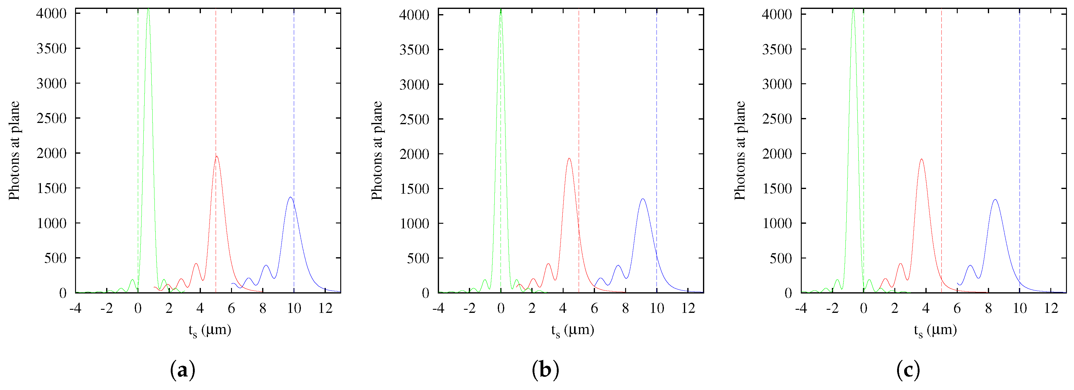
The first step in this study was the computational implementation of the Gibson and Lanni theoretical PSF model [13]. This is a computationally-convenient scalar model that represents appropriately the spherical aberration produced by using a microscope system under non-design conditions. The optical sectioning technique is an example of this use in which, in the best scenario, the spherical aberration depends only on the depth of the fluorescent point source. In this case, the model appropriately describes the 3D PSF and evidences a strong spatial variance in the optical axis, showing at least three effects easily viewed in an intensity profile: morphology changes, including asymmetry relative to the peak, intensity changes and focal shift of the 3D PSF. This last effect reveals that the axial positions of the focused structures in images acquired by optical sectioning are not necessarily coincident with the positions directly measured from the relative distance between the cover slip and the objective lens. Therefore, in real situations where other factors are involved, it is practically impossible to know with certainty the spatial position from direct measurement between glasses and the objective lens. In fact, any small change in other parameters of the model (e.g., refraction index of immersion oil $n_{oil}$) produces a different shift (Figure 12). In this sense, Rees et al. [19] have recently arrived at the same conclusion in their analysis, which included those modes of superresolution microscopy that use conventional fluorescence microscopes. In turn, this shows that estimators obtained via the sampling theory can be sufficient to provide useful information about precision and resolution. This highlights the importance of the estimation methods and the selection of an adequate image formation model for localization and deconvolution applications [16,17,37].

Regarding deconvolution, a valid concern could come up for users. If the parameter estimation methods are performed over a limited axial support, what would its validity be for the larger PSF extension needed for deconvolution? It is still valid, because it is possible to have a good estimation of the PSF parameters with a smaller extension than the one used in restoration. In fact, according to the results obtained, using data from the optical axis would be enough for a good estimation of the axial position of the PSF, which, depending on the signal level, could even be in the nanometer order. Thus, parameter estimation methods could be applied to a reduced dataset to find the optimal PSF before restoration. This would need less computation time than using the full 3D PSF dataset.

5.2. Computational Convergence

Regarding method convergence, it is necessary to point out that the numerical optimization method has a theoretical quadratic convergence. However, the tests carried out on simulated images, with and without noise, showed a logarithmic linear convergence (Table 2) of the estimation methods considered here. A downside of the approximation method used for optimization, also discussed by Aguet et al. [10], is that it requires a good initial estimate. The speed of the estimation methods could be improved taking into account more terms of the Taylor representation of the optimization method. However, this would require an additional performance evaluation because there might be more computations of the model due to the use of higher order derivatives.

5.3. General Performance of Methods

The analysis of success percentage was shown to be a useful tool for comparative analysis of the methods. Users could be confident that the methods are achieving good accuracy and precision, but this could not have any statistical value, since the chance of success could have low probability. This situation became evident with the results obtained using sagittal slices. In these cases, both CRBs as estimation methods were shown to be better than those obtained with optical sections for the same photon count. However, more photon counting is required for the sagittal slice to have a more reasonable success percentage in comparison with the optical section at −1 $\mathsf{\mu }$m, for example. In this sense, it should be noted that the CRB establishes a bound to the variance of the unbiased estimator, but nothing can be deduced from the method by which the estimator is computed. This assigns a truly methodological importance to the simulation. It could be argued that the range of initial estimates is wide and that the success percentage would increase making it narrower. The argument is valid in the theoretical sense, in the same way that the success percentage will improve when the photon count increases. However, in practical applications, the range of the initial estimates is limited by the real information of the parameter to be estimated. In fact, the range of initial estimates of the sagittal slice is less than the one used for optical sections, since using the same range, the results obtained were much less satisfying than the ones presented in the last rows of Figure 5, Figure 6, Figure 7, Figure 8 and Figure 9.

Our results indicate that the estimation of the axial position using the Gibson and Lanni model requires a high SNR to achieve $95\%$ of success and higher still to be close to the CRB. In fact, only the ML and MIDIV methods (last row of Figure 10) achieved the theoretical precision given by the CRB when data collected from the optical axis were used. A test done using more −DF optical sections did not improve the precision shown in the first row of Figure 9. However, it must be noted that, in practice, exposition time is generally fixed during optical sectioning acquisition; thus, the more DF the optical section acquired is, the less the photon count will be.

The incidence of the extrinsic noise sources (NCII or NCIII) showed that success percentage estimation worsened, but no difference was found between noise sources. In fact, when columns NCII and NCIII of Figure 5, Figure 6, Figure 7, Figure 8 and Figure 9 are compared, the qualitative result is very similar. In other words, estimation methods have the chance to successfully converge in cases where there are additive noise sources not considered in the forward model.

Finally, a reference to the MIDIV, our own method, is required. In this approach, there were no assumptions about noise, which is an advantage over ML and LSQR. It also should be noted that MIDIV has achieved the CRB in similar conditions to ML. However, a strong hypothesis was made about the experimental PSF representing a probability density in accordance with the law of large numbers. This assumption is true when the photon number tends to infinity, which does not hold in practice. In real circumstances, the number of photons is finite, and the variability of the mean level of intensity in each pixel is different. In pixels that capture the PSF peak, the variability of the mean level of intensity is less than in those that capture darker areas of the PSF. This may be influencing the method’s performance.

5.4. Test with an Experimental PSF

Estimations using an experimental PSF showed similar qualitative results. FWHM in both lateral and axial directions were evaluated, and all methods showed the same results up to the third decimal (nanometer). However, to obtain a sounder conclusion in this aspect, it is necessary to run a more complete and controlled experiment, which is beyond the purpose of this work.

6. Conclusions

Optical sectioning is, without corrected optics for this purpose, a shift-variant tomographic technique. In the best case, this is due to the spherical aberration that depends only on the light source position along the optical axis.

The Gibson and Lanni model appropriately predicts the 3D PSF for optical sectioning, evidencing changes in morphology and intensity, as well as focal shift.

Parameter estimation methods can be used together with the Gibson and Lanni model to efficiently estimate the position of a point light source along the optical axis from experimental data.

The iterative forms of the three parameter estimation methods tested in this work showed logarithmic linear convergence.

The estimation of the axial position using the Gibson and Lanni model requires a high SNR to achieve $95\%$ of success and higher still to be close to the CRB.

ML achieved a higher success percentage at lower signal levels compared with MIDIV and LSQR for the intrinsic noise source NCI.

Only the ML and MIDIV methods achieved the theoretical precision given by the CRB, but only with data belonging to the optical axis and high SNR.

Extrinsic noise sources NCII and NCII worsened the success percentage of all methods, but no difference was found between noise sources for the same method, for all methods studied.

The success percentage and CRB analysis are useful and necessary tools for comparative analysis of estimation methods. They are also useful for simulation before experimental applications.

References

1. Wu, Q.; Merchant, F.A.; Castleman, K.R. Microscope Image Processing; Academic Press: New York, NY, USA, 2008. [Google Scholar]
2. Jansson, P. (Ed.) Deconvolution of Images and Spectra, 2nd ed.; Academic Press: Chestnut Hill, MA, USA, 1997.
3. Deschout, H.; Zanacchi, F.C.; Mlodzianoski, M.; Diaspro, A.; Bewersdorf, J.; Hess, S.T.; Braeckmans, K. Precisely and accurately localizing single emitters in fluorescence microscopy. Nat. Methods 2014, 11, 253–266. [Google Scholar] [CrossRef] [PubMed]
4. Sanchez-Beato, A.; Pajares, G. Noniterative Interpolation-Based Super-Resolution Minimizing Aliasing in the Reconstructed Image. IEEE Trans. Image Process. 2008, 17, 1817–1826. [Google Scholar] [CrossRef] [PubMed]
5. DeSantis, M.C.; Zareh, S.K.; Li, X.; Blankenship, R.E.; Wang, Y.M. Single-image axial localization precision analysis for individual fluorophores. Opt. Express 2012, 20, 3057–3065. [Google Scholar] [CrossRef] [PubMed]
6. Sarder, P.; Nehorai, A. Deconvolution methods for 3-D fluorescence microscopy images. IEEE Signal Process. Mag. 2006, 23, 32–45. [Google Scholar] [CrossRef]
7. Rieger, B.; Nieuwenhuizen, R.; Stallinga, S. Image Processing and Analysis for Single-Molecule Localization Microscopy: Computation for nanoscale imaging. IEEE Signal Process. Mag. 2015, 32, 49–57. [Google Scholar] [CrossRef]
8. Ober, R.; Tahmasbi, A.; Ram, S.; Lin, Z.; Ward, E. Quantitative Aspects of Single-Molecule Microscopy: Information-theoretic analysis of single-molecule data. IEEE Signal Process. Mag. 2015, 32, 58–69. [Google Scholar] [CrossRef] [PubMed]
9. Hanser, B.M.; Gustafsson, M.G.L.; Agard, D.A.; Sedat, J.W. Phase-retrieved pupil functions in wide-field fluorescence microscopy. J. Microsc. 2004, 216, 32–48. [Google Scholar] [CrossRef] [PubMed]
10. Aguet, F.; van de Ville, D.; Unser, M. A maximum-likelihood formalism for sub-resolution axial localization of fluorescent nanoparticles. Opt. Express 2005, 13, 1–20. [Google Scholar] [CrossRef]
11. Mortensen, K.I.; Churchman, L.S.; Spudich, J.A.; Flyvbjerg, H. Optimized localization analysis for single-molecule tracking and super-resolution microscopy. Nat. Methods 2010, 7, 377–381. [Google Scholar] [CrossRef] [PubMed]
12. Kirshner, H.; Aguet, F.; Sage, D.; Unser, M. 3-D PSF fitting for fluorescence microscopy: Implementation and localization application. J. Microsc. 2013, 249, 13–25. [Google Scholar] [CrossRef] [PubMed]
13. Gibson, S.F.; Lanni, F. Experimental test of an analytical model of aberration in an oil-immersion objective lens used in three-dimensional light microscopy. J. Opt. Soc. Am. A 1991, 8, 1601–1613. [Google Scholar] [CrossRef]
14. Cheezum, M.K.; Walker, W.F.; Guilford, W.H. Quantitative comparison of algorithms for tracking single fluorescent particles. Biophys. J. 2001, 81, 2378–2388. [Google Scholar] [CrossRef]
15. Abraham, A.V.; Ram, S.; Chao, J.; Ward, E.S.; Ober, R.J. Quantitative study of single molecule location estimation techniques. Opt. Express 2009, 17, 23352–23373. [Google Scholar] [CrossRef] [PubMed]
16. Kim, B.; Naemura, T. Blind Depth-variant Deconvolution of 3D Data in Wide-field Fluorescence Microscopy. Sci. Rep. 2015, 5, 9894. [Google Scholar] [CrossRef] [PubMed]
17. Kim, B.; Naemura, T. Blind deconvolution of 3D fluorescence microscopy using depth-variant asymmetric PSF. Microsc. Res. Tech. 2016, 79, 480–494. [Google Scholar] [CrossRef] [PubMed]
18. Shaevitz, J.W. Bayesian Estimation of the Axial Position in Astigmatism-Based Three-Dimensional Particle Tracking. Int. J. Opt. 2009, 2009, 896208. [Google Scholar] [CrossRef]
19. Rees, E.J.; Erdelyi, M.; Pinotsi, D.; Knight, A.; Metcalf, D.; Kaminski, C.F. Blind assessment of localisation microscope image resolution. Opt. Nanosc. 2012, 1, 12. [Google Scholar] [CrossRef]
20. Cox, S.; Rosten, E.; Monypenny, J.; Jovanovic-Talisman, T.; Burnette, D.T.; Lippincott-Schwartz, J.; Jones, G.E.; Heintzmann, R. Bayesian localization microscopy reveals nanoscale podosome dynamics. Nat. Methods 2012, 9, 195–200. [Google Scholar] [CrossRef] [PubMed]
21. Walde, M.; Monypenny, J.; Heintzmann, R.; Jones, G.E.; Cox, S. Vinculin Binding Angle in Podosomes Revealed by High Resolution Microscopy. PLoS ONE 2014, 9, e88251. [Google Scholar] [CrossRef] [PubMed]
22. Goodman, J.W. Introduction to Fourier Optics (Electrical and Computer Engineering), 2nd ed.; McGraw-Hill: New York, NY, USA, 1996. [Google Scholar]
23. Castleman, K.R. Digital Image Processing; Prentice Hall: Englewood Cliffs, NJ, USA, 1996. [Google Scholar]
24. Snyder, D.L.; Hammoud, A.M.; White, R.L. Image recovery from data acquired with a charge-coupled-device camera. J. Opt. Soc. Am. A 1993, 10, 1014–1023. [Google Scholar] [CrossRef] [PubMed]
25. Frieden, B.R. Probability, Statistical Optics, and Data Testing. A Problem Solving Approach; Springer: Berlin/Heidelberg, Germany, 2001. [Google Scholar]
26. Eaton, J.W.; Bateman, D.; Hauberg, S. GNU Octave Version 3.0.1 Manual: A High-Level Interactive Language for Numerical Computations; CreateSpace Independent Publishing Platform: North Charleston, SC, USA, 2009. [Google Scholar]
27. Shampine, L. Vectorized adaptive quadrature in {MATLAB}. J. Comput. Appl. Math. 2008, 211, 131–140. [Google Scholar] [CrossRef]
28. Dunn, S.M.; Constantinides, A.; Moghe, P.V. Numerical Methods in Biomedical Engineering; Academic Press: New York, NY, USA, 2006. [Google Scholar]
29. Wang, Z.; Bovik, A. Mean squared error: Love it or leave it? A new look at Signal Fidelity Measures. IEEE Signal Process. Mag. 2009, 26, 98–117. [Google Scholar] [CrossRef]
30. Csiszar, I. Why Least Squares and Maximum Entropy? An Axiomatic Approach to Inference for Linear Inverse Problems. Ann. Stat. 1991, 19, 2032–2066. [Google Scholar] [CrossRef]
31. Snyder, D.; Schulz, T.; O’Sullivan, J. Deblurring subject to nonnegativity constraints. IEEE Trans. Signal Process. 1992, 40, 1143–1150. [Google Scholar] [CrossRef]
32. Montgomery, D.; Runger, G.; You, H. Applied Statistics and Probability for Engineers, Student Workbook with Solutions; John Wiley & Sons: New York, NY, USA, 2003. [Google Scholar]
33. Efron, B.; Tibshirani, R.J. An Introduction to the Bootstrap; Number 57 in Monographs on Statistics and Applied Probability; Chapman & Hall/CRC: London, UK, 1993. [Google Scholar]
34. Aguet, F.; van de Ville, D.; Unser, M. An accurate PSF model with few parameters for axially shift-variant deconvolution. In Proceedings of the 5th IEEE International Symposium on Biomedical Imaging: From Nano to Macro (ISBI 2008), Paris, France, 14–17 May 2008; pp. 157–160.
35. Diaz-Zamboni, J.E.; Adur, J.F.; Osella, D.; Izaguirre, M.F.; Casco, V.H. Software para usuarios de microscopios de desconvolución digital. In Proceedings of the XV Congreso Argentino de Bioingeniería, Paraná, Brazil, 21–23 September 2005.
36. Adur, J.F.; Diaz Zamboni, J.E.; Vicente, N.B.; Izaguirre, M.F.I.; Casco, V.H. Digital Deconvolution Microscopy: Development, Evaluation and Utilization in 3D quantitative studies of E-cadherin expression in skin of Bufo arenarun tadpoles. In Modern Research and Educational Topics in Microscopy, 3rd ed.; Microscopy Book Series; Chapter Techniques; Méndez-Vilas, A., Díaz, J., Eds.; Formatex: Badajoz, Spain, 2007; Volume 2, pp. 906–916. [Google Scholar]
37. Ghosh, S.; Preza, C. Fluorescence microscopy point spread function model accounting for aberrations due to refractive index variability within a specimen. J. Biomed. Opt. 2015, 20, 075003. [Google Scholar] [CrossRef] [PubMed]
Figure 1. Path ray scheme for design and non-design conditions.
Jimaging 03 00007 g001
Figure 2. Cramer–Rao lower bound computed with Equation (20) for the noisy point spread function (PSF) model given by Equation (5) under several acquisition conditions. In black, the theoretical PSF intensity axial profile for reference. (a) CRB versus photon number; (b) CRB versus background; (c) CRV versus pixel number; (d) CRB versus pixel size.
Jimaging 03 00007 g002
Figure 3. Descriptive statistics of the residuals of initial estimates and estimations of the methods. Residuals of initial estimates where computed as the absolute value of the difference between the randomized initial estimate and the ground truth. (a) Without noise; (b) Noise Case I (NCI); (c) NCII; (d) NCIII.
Jimaging 03 00007 g003aJimaging 03 00007 g003b
Figure 4. Samples of diffracted-limited images obtained from the Gibson and Lanni model [13] are shown in the column marked (a). The same images degraded by different noise conditions are shown in the columns marked (bd). The last row depicts the samples of sagittal slices. (a) Without noise; (b) NCI; (c) NCII; (d) NCIII.
Jimaging 03 00007 g004
Figure 5. Success measurements of the methods: MIDIV (red), ML (green) and LSQR (blue). A dashed line at 95 % has been plotted in all subfigures for reference. Estimation results are presented as the mean point estimates of the success percentages and their confidence intervals. (a) NCI; (b) NCII; (c) NCIII.
Jimaging 03 00007 g005
Figure 6. Iteration measurements of the methods: MIDIV (red), ML (green) and LSQR (blue). Iteration number results are presented as the mean point estimates of the iteration number and their confidence intervals. (a) NCI; (b) NCII; (c) NCIII.
Jimaging 03 00007 g006
Figure 7. Time measurements of the methods: MIDIV (red), ML (green) and LSQR (blue). Results are presented as the mean point estimates of the total computing times per parameter estimation and their confidence intervals. (a) NCI; (b) NCII; (c) NCIII.
Jimaging 03 00007 g007
Figure 8. Accuracy measurements of methods: MIDIV (red), ML (green) and LSQR (blue). The dashed line at 5 μ m represents the ground truth (GT), the actual value of the parameter from which data were generated. The results of accuracy are presented as the mean point estimates of the set of estimations of t s and their confidence intervals. (a) NCI; (b) NCII; (c) NCIII.
Jimaging 03 00007 g008
Figure 9. Precision measurements of the methods: MIDIV (red), ML (green) and LSQR (blue). The dashed line represents the theoretical standard deviation of the initial estimates ( σ I E s ). The Cramer–Rao bound (CRB) is shown in solid line segments for each level of intensity. Precision results are presented as the point estimates of the standard deviations of the t s estimations and their confidence intervals. (a) NCI; (b) NCII; (c) NCIII.
Jimaging 03 00007 g009
Figure 10. Optical axis estimation results of the methods: MIDIV (red), ML (green) and LSQR (blue). (a) NCI; (b) NCII; (c) NCIII.
Jimaging 03 00007 g010
Figure 11. Pseudocolor images of 45 × 31 pixels. Upper left, image of fluorescent nanobead of 0.170 ± 0.005 μ m in diameter. In the counter clockwise direction: synthetic PSFs obtained by the estimations of the axial t s by MIDIV, LSQR and ML, respectively.
Jimaging 03 00007 g011
Figure 12. Intensity profiles along the optical axis of the Gibson and Lanni model. Green profiles, t s = 0 μ m; blue profiles, t s = 3 μ m; and red profiles, t s = 10 μ m. Center image, n o i l in the design condition; left and right plots, n o i l in the non-design conditions. (a) n o i l = 1 . 510 ; (b) n o i l = 1 . 515 ; (c) n o i l = 1 . 520 .
Jimaging 03 00007 g012