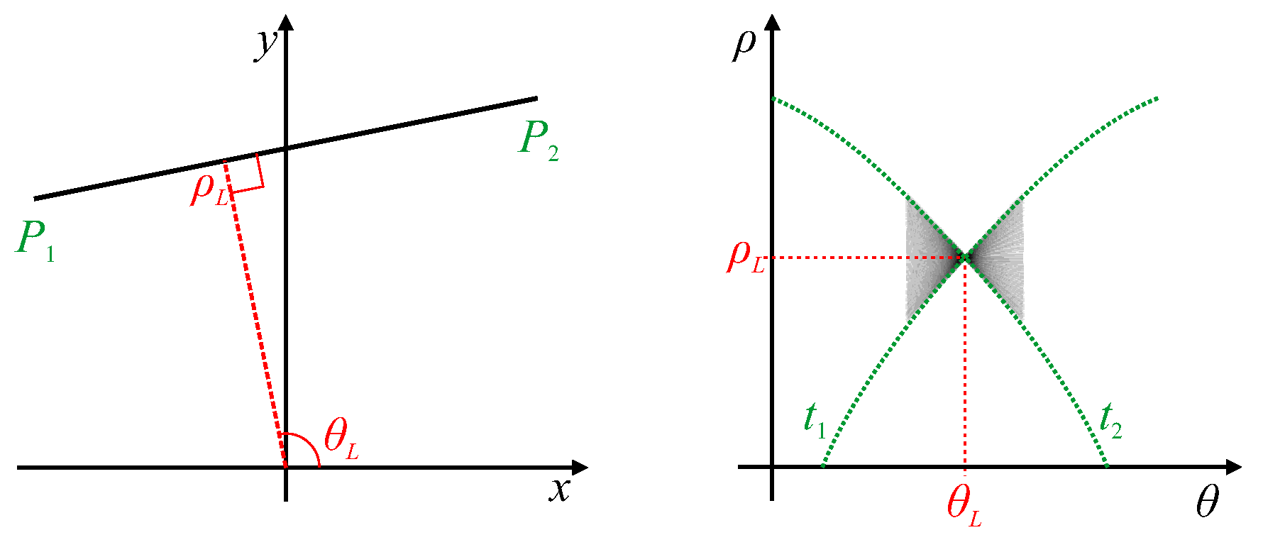
Figure 1.
Superposition of traces resulting in a butterfly pattern in the vicinity of a peak. Points and are the endpoints of a line segment, and generate traces and which bound the butterfly located at .
Figure 1.
Superposition of traces resulting in a butterfly pattern in the vicinity of a peak. Points and are the endpoints of a line segment, and generate traces and which bound the butterfly located at .
Figure 2.
A curved line and its corresponding original Hough transform. Points and are the endpoints of the curved line, with generated traces and bounding the butterfly. L represents the curved locus of peak votes resulting from changes in slope along the curved line.
Figure 2.
A curved line and its corresponding original Hough transform. Points and are the endpoints of the curved line, with generated traces and bounding the butterfly. L represents the curved locus of peak votes resulting from changes in slope along the curved line.
Figure 3.
Gradient Hough transform; point with gradient maps to point in parameter space.
Figure 3.
Gradient Hough transform; point with gradient maps to point in parameter space.
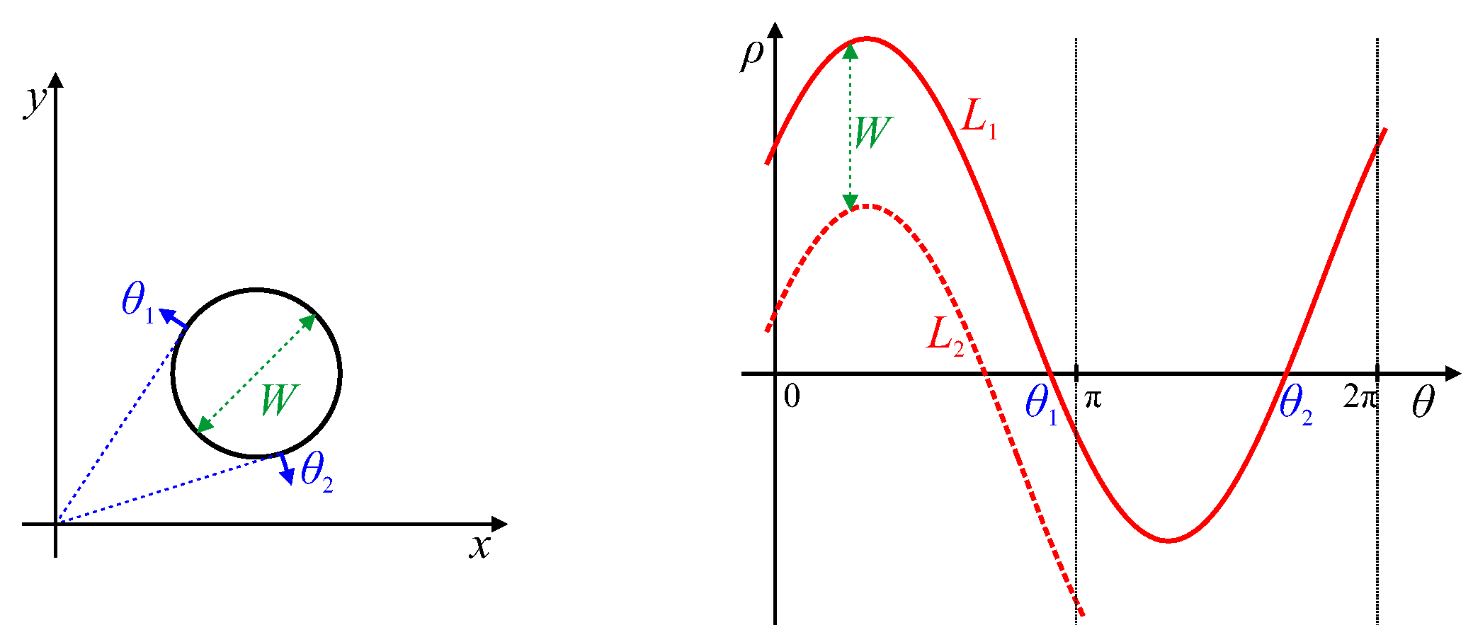
Figure 4.
Line Hough transform of a closed curve. The red locus,
, covers the range
. Zero crossings
and
correspond to tangents through the origin. When the sign of the edge is unimportant, the section
can be mapped to the range
using Equation (
9), as shown by the dashed locus,
.
Figure 4.
Line Hough transform of a closed curve. The red locus,
, covers the range
. Zero crossings
and
correspond to tangents through the origin. When the sign of the edge is unimportant, the section
can be mapped to the range
using Equation (
9), as shown by the dashed locus,
.
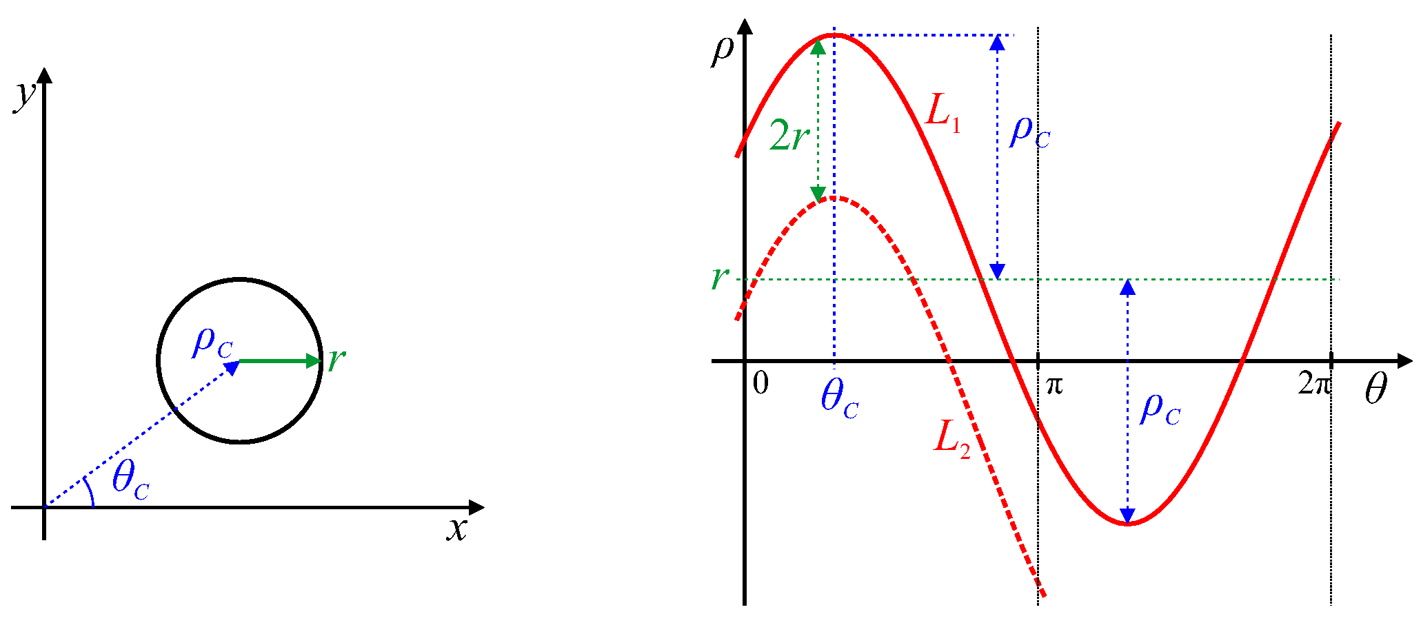
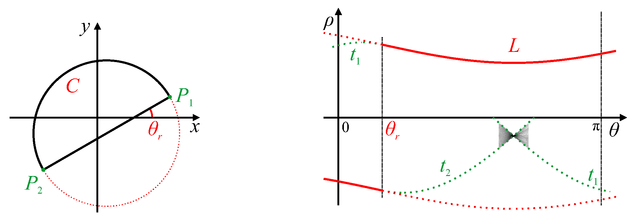
Figure 5.
Hough transform of a circular curve of radius r. Key features of the parameter locus are marked.
Figure 5.
Hough transform of a circular curve of radius r. Key features of the parameter locus are marked.
Figure 6.
The Hough transform of an elliptical curve generates the parameter locus,
. Constructions from
are shown for deriving the five ellipse parameters.
is
inverted and offset by
. The Feret diameter,
, shown in green, is the difference between
and
from Equation (
10). The major and minor axes and ellipse orientation,
, are derived from this as marked. The centre curve,
, in blue, is the average of
and
from Equation (
11), with the ellipse centre parameters marked.
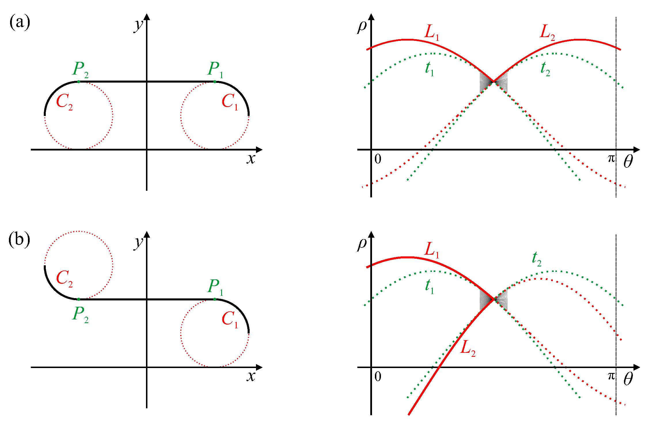
Figure 7.
Hough transform of a linear segment with curves at each end. Traces and , generated by segment endpoints and , respectively, bound the butterfly. Circular arcs and at each end of the line segment generate parameter loci and , respectively. Case (a): The slope of the curve continues, thus the loci leave opposite sides of the butterfly. Case (b): The slope of the curve changes back, thus the loci leave the same side of the butterfly.
Figure 8.
Inflection points and on the edge result in the locus doubling back with the same slope, generating cusps (labelled and , respectively) in parameter space. Circular arcs to generate parameter loci to , respectively; the dotted lines in parameter space represent the extension of the loci if the edge continued following the arcs.
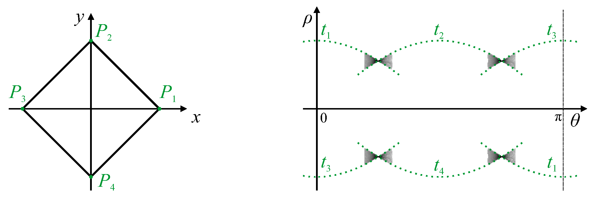
Figure 9.
Hough transform of an object with corners. Corner points to have corresponding traces to . Butterflies at the intersection of traces correspond to the linear segments between corners. Note that, with the gradient Hough transform, the traces between the butterflies will not actually receive any votes; they are drawn here to illustrate the relationship between the bounding edges of the butterflies.
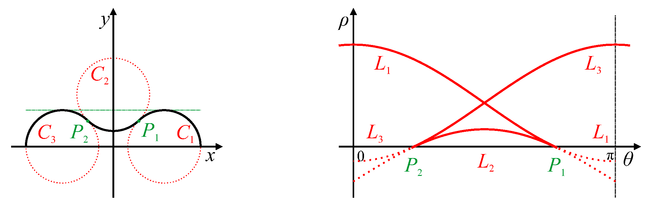
Figure 10.
Hough transform of a semi-circle with corners. Corner points and have corresponding traces and (shown dotted because the sharp corners will not result in votes with the gradient Hough transform). The peak of the butterfly gives the parameters of the line connecting and . The circular segment, C, generates the peak locus, L (the dotted segment corresponds to the locus of the truncated circular segment in the image).
Figure 11.
Hough transform of two intersecting circles. The circular arcs and map to the peak loci and , respectively (with the dotted segments of L corresponding to the dotted segments of C). Corner points and have corresponding traces and (shown dotted because they will receive no votes in the gradient Hough transform).
Figure 12.
Selecting only the maximum and minimum locus for each angle gives the convex hull of the shape. Convex intersection points and correspond to lines and within the image which are the convex edges that span the concavities. The depth of the concavity is d.
Figure 12.
Selecting only the maximum and minimum locus for each angle gives the convex hull of the shape. Convex intersection points and correspond to lines and within the image which are the convex edges that span the concavities. The depth of the concavity is d.
Figure 13.
A parabolic curve, C, and its corresponding peak locus, L, in the original Hough transform. Traces and are generated from endpoints and , respectively (these may be the edges of the image). Parabola parameters and map directly to features of the locus. The quadratic parameter, , of C is also reflected directly in the quadratic parameter of L.
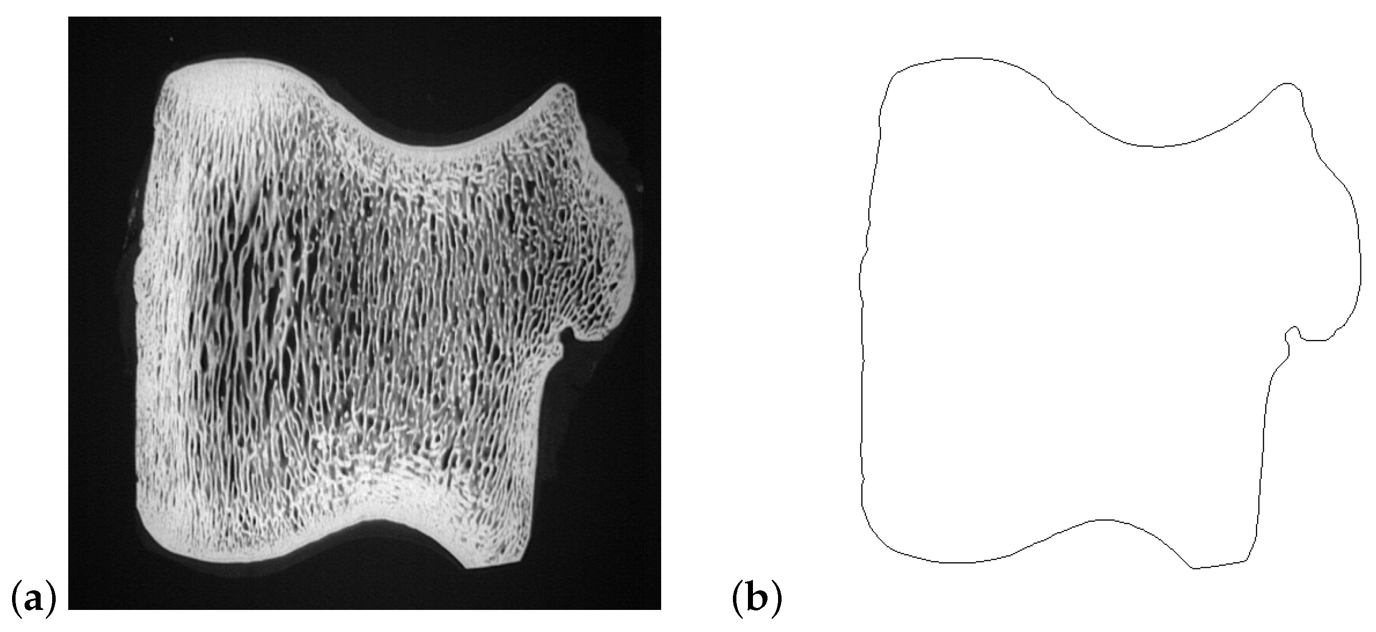
Figure 14.
Example of processing an image with a complex shape: (a) the image; and (b) outline of the image detected by the Canny filter.
Figure 14.
Example of processing an image with a complex shape: (a) the image; and (b) outline of the image detected by the Canny filter.
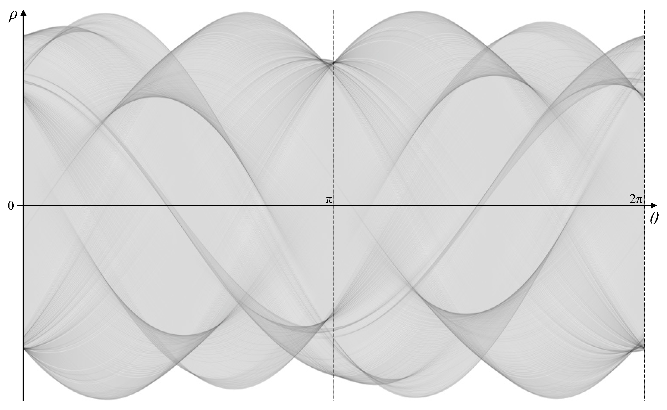
Figure 15.
The full Hough transform of the boundary from
Figure 14 (contrast enhanced for visibility).
Figure 15.
The full Hough transform of the boundary from
Figure 14 (contrast enhanced for visibility).
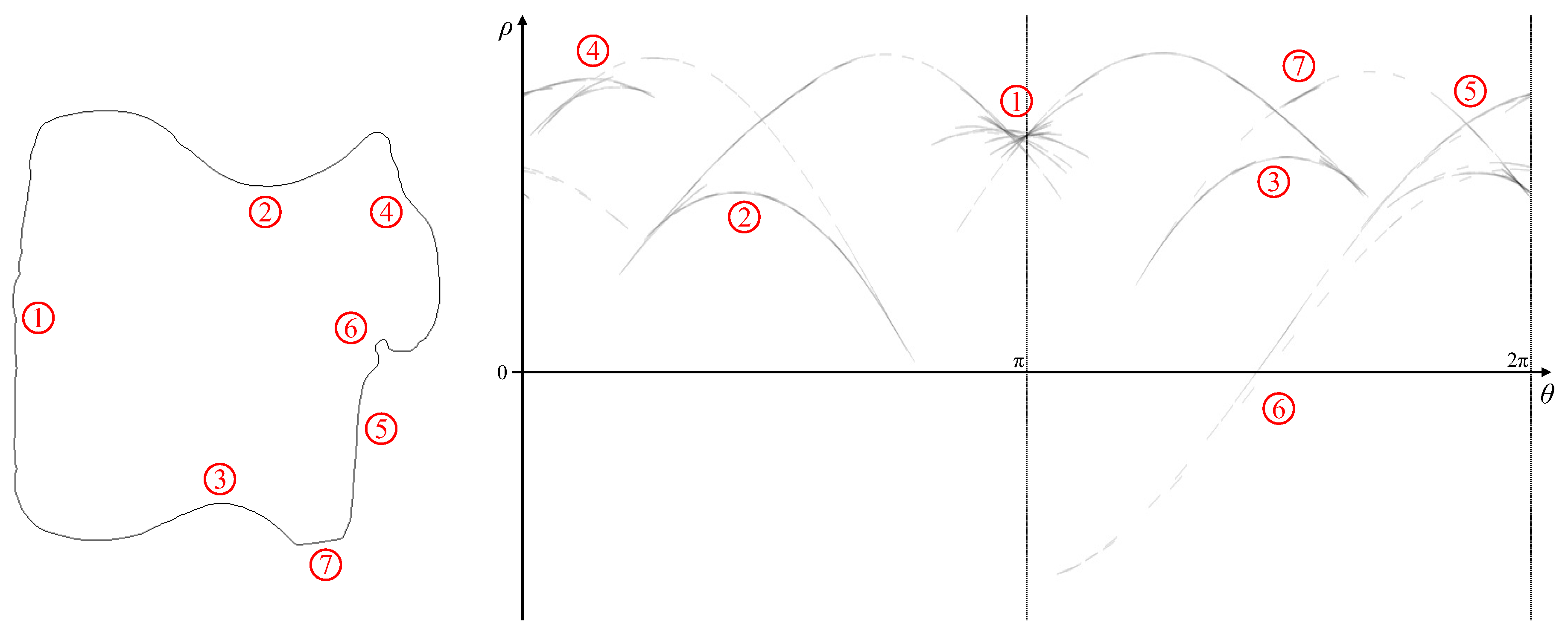
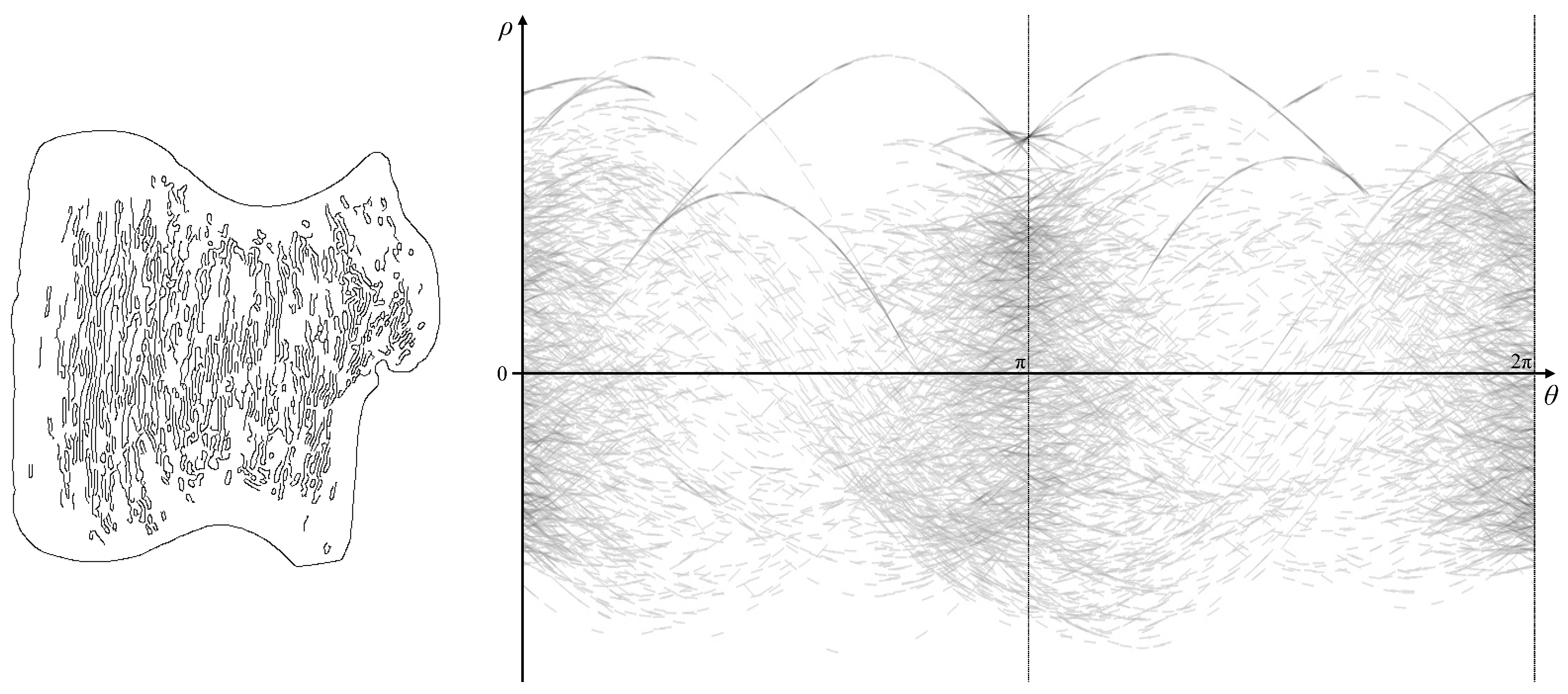
Figure 16.
The shape and its pattern in parameter space after the gradient Hough transform (contrast enhanced for visibility). Numbered features link the patterns with the corresponding regions on the object shape.
Figure 16.
The shape and its pattern in parameter space after the gradient Hough transform (contrast enhanced for visibility). Numbered features link the patterns with the corresponding regions on the object shape.
Figure 17.
The underlying peak locus from the Hough transform in
Figure 16 (obtained using Algorithm 3, not derived from the previous figure).
Figure 17.
The underlying peak locus from the Hough transform in
Figure 16 (obtained using Algorithm 3, not derived from the previous figure).
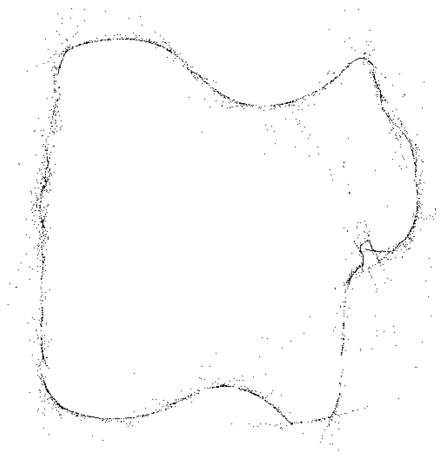
Figure 18.
Simple reconstruction of the boundary points (using Algorithm 4).
Figure 18.
Simple reconstruction of the boundary points (using Algorithm 4).
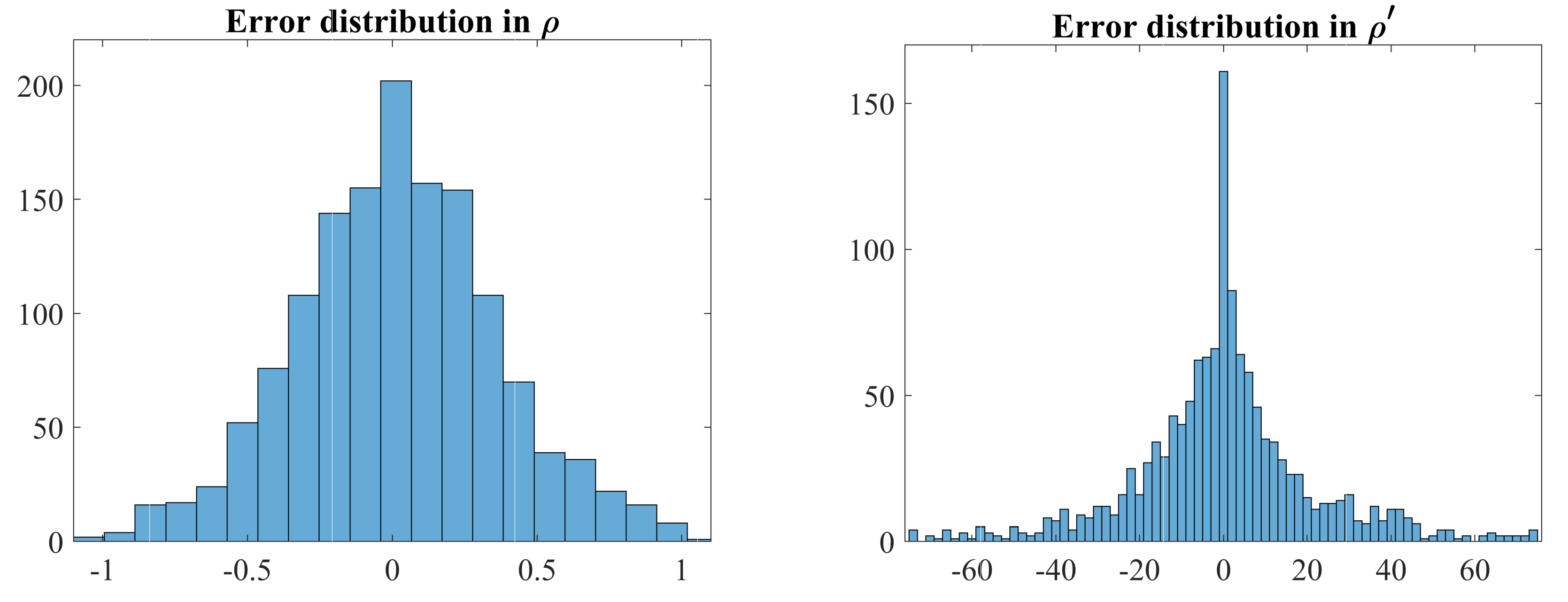
Figure 19.
Error distributions of measured values of and from the Hough transform. Standard deviations are pixels and pixels/radian.
Figure 19.
Error distributions of measured values of and from the Hough transform. Standard deviations are pixels and pixels/radian.
Figure 20.
Filtered reconstruction of the boundary points. (a) Linked edge points (without filtering), clearly showing outliers. (b) After filtering successive points using a cosine similarity score; remaining significant noise on the boundary is highlighted.
Figure 20.
Filtered reconstruction of the boundary points. (a) Linked edge points (without filtering), clearly showing outliers. (b) After filtering successive points using a cosine similarity score; remaining significant noise on the boundary is highlighted.
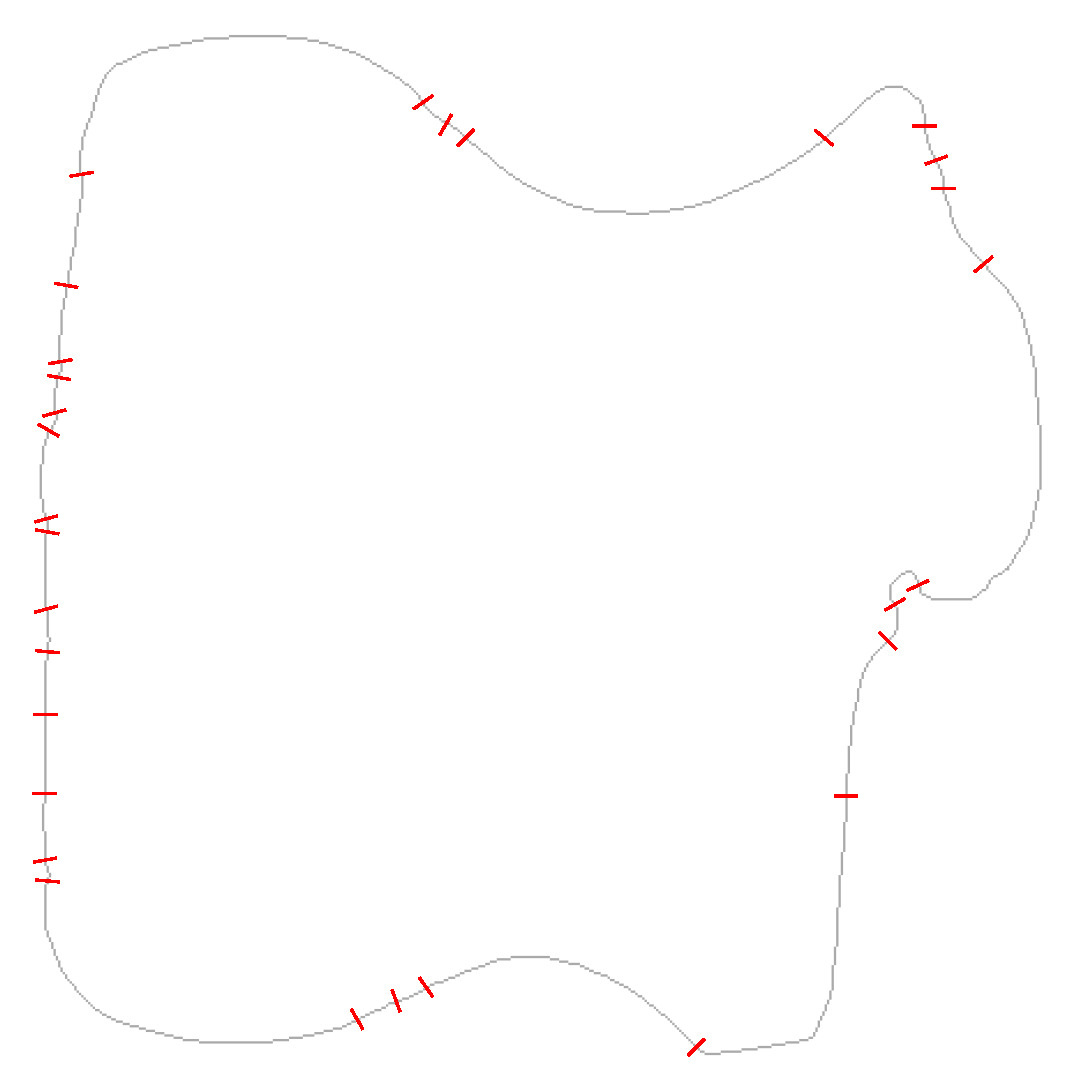
Figure 21.
Inflection points marked on the original image, as detected from the Hough transform.
Figure 21.
Inflection points marked on the original image, as detected from the Hough transform.
Figure 22.
Convex hull, uses the outermost peak locus. The reconstructed convex hull is shown on the right superimposed in red on the original outline.
Figure 22.
Convex hull, uses the outermost peak locus. The reconstructed convex hull is shown on the right superimposed in red on the original outline.
Figure 23.
The shape with all edges present, and its corresponding gradient Hough transform (contrast enhanced for visibility).
Figure 23.
The shape with all edges present, and its corresponding gradient Hough transform (contrast enhanced for visibility).
Figure 24.
The shape with detected edges, and its corresponding gradient Hough transform (contrast enhanced for visibility).
Figure 24.
The shape with detected edges, and its corresponding gradient Hough transform (contrast enhanced for visibility).
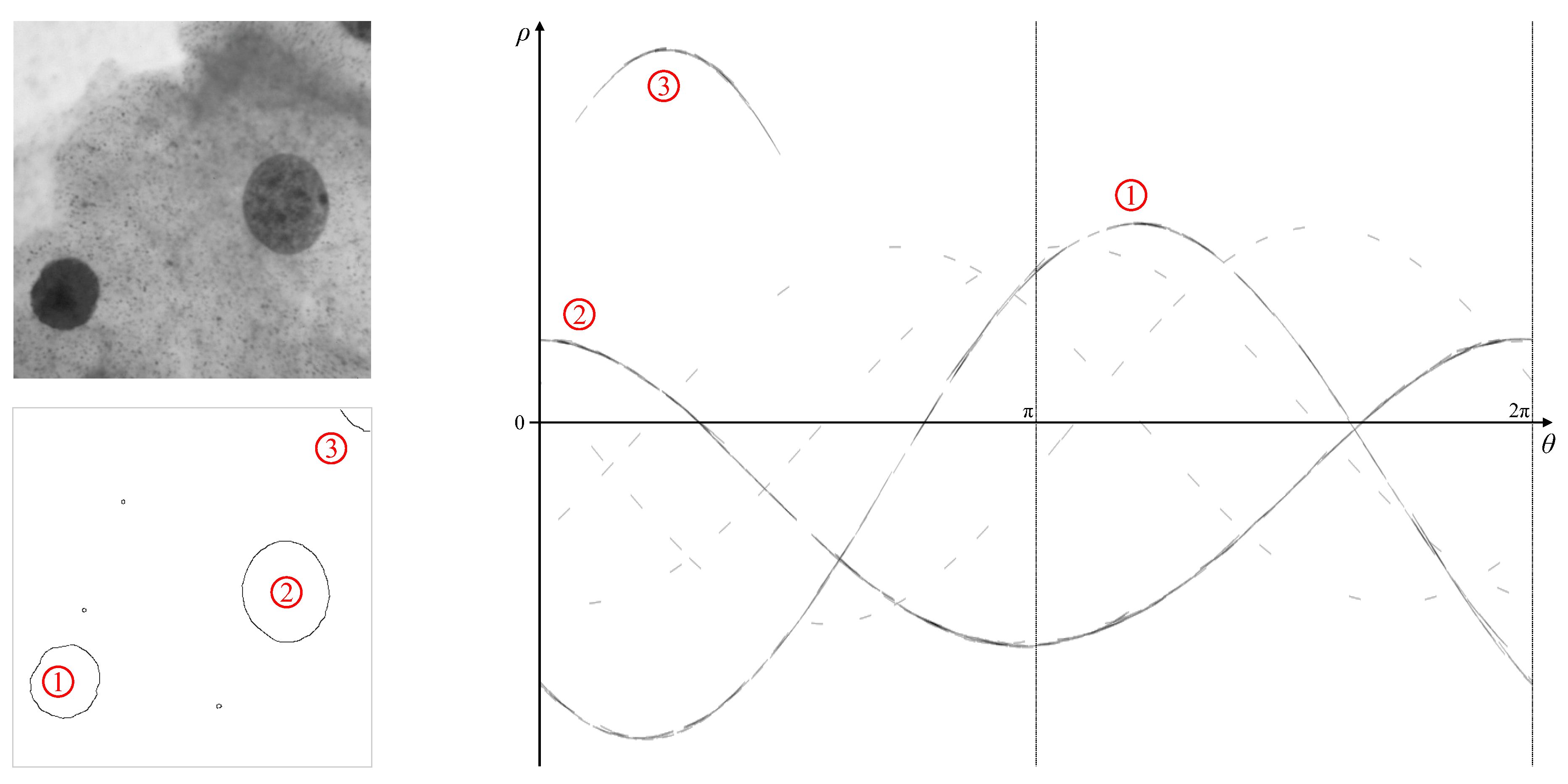
Figure 25.
Using the parameter loci to derive parameters of the elliptical objects. The flipped locus,
in Equation (
9), centre line,
C in Equation (
11), and the Feret diameter,
W in Equation (
10), are shown for each of the two blobs. The blue, yellow and green dotted lines correspond to the detected feature points on the curves for object centre, major diameter and minor diameter, respectively.
Figure 26.
Detected elliptical objects. The blue line shows the object position relative to the image centre, with the yellow and green lines showing the major and minor diameters.
Figure 26.
Detected elliptical objects. The blue line shows the object position relative to the image centre, with the yellow and green lines showing the major and minor diameters.


