
Improving Scene Text Recognition for Indian Languages with Transfer Learning and Font Diversity


Abstract
:1. Introduction
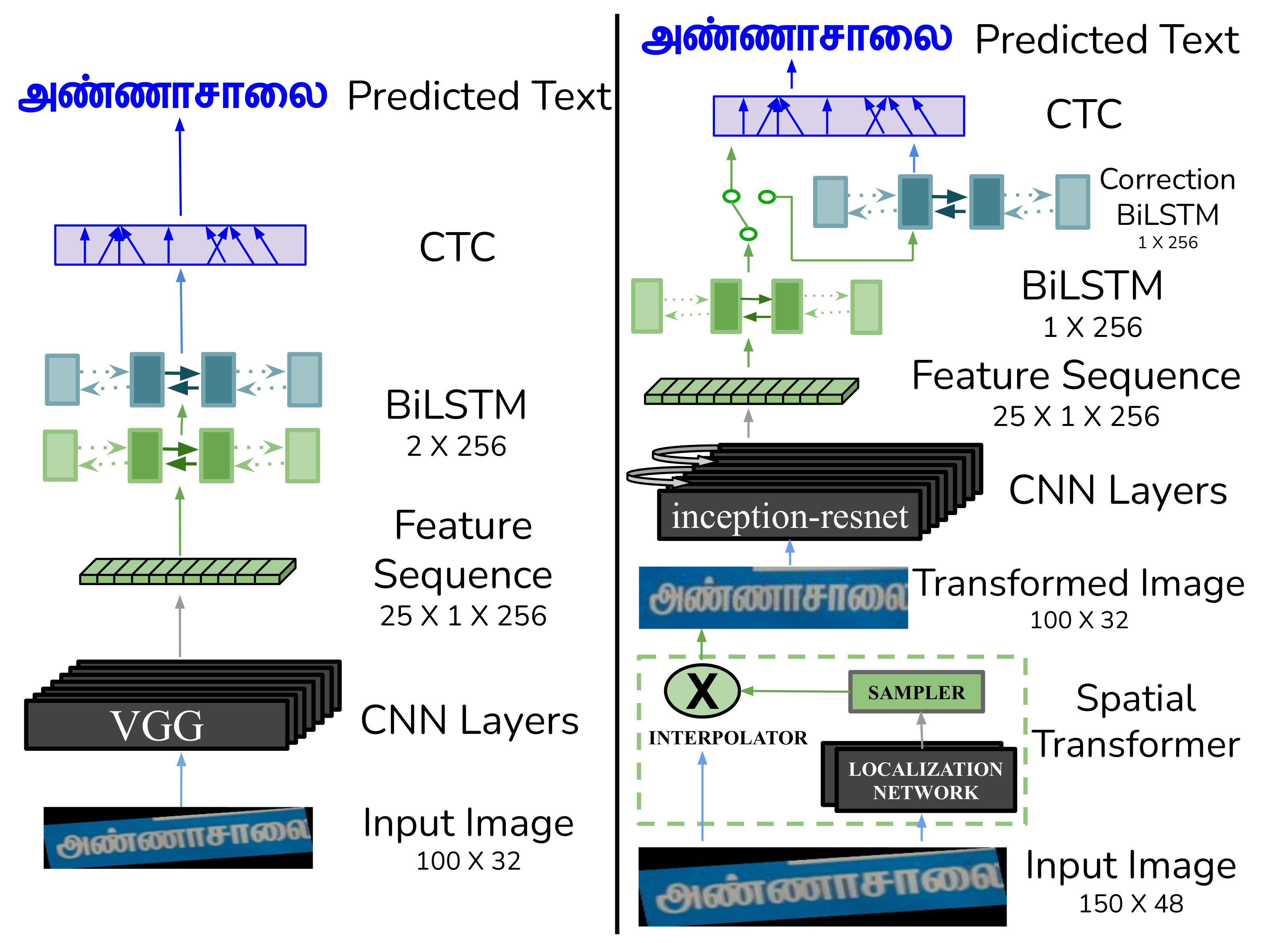
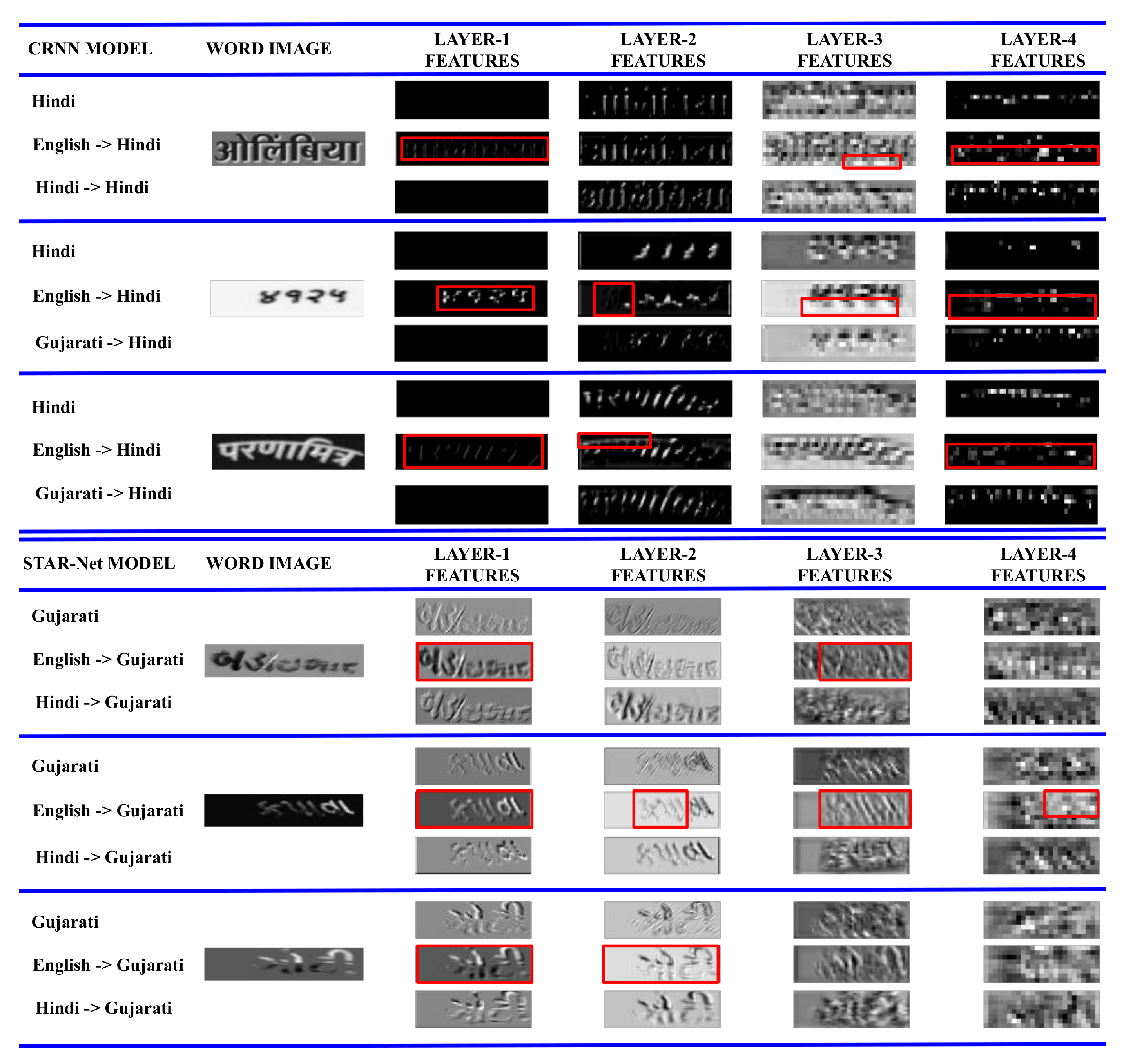
- We investigate the transfer learning of complete scene-text recognition models—(i) from English to two Indian languages (Hindi and Gujarati) and (ii) among the six Indian languages, i.e., Gujarati, Hindi, Bangla, Telugu, Tamil, and Malayalam.
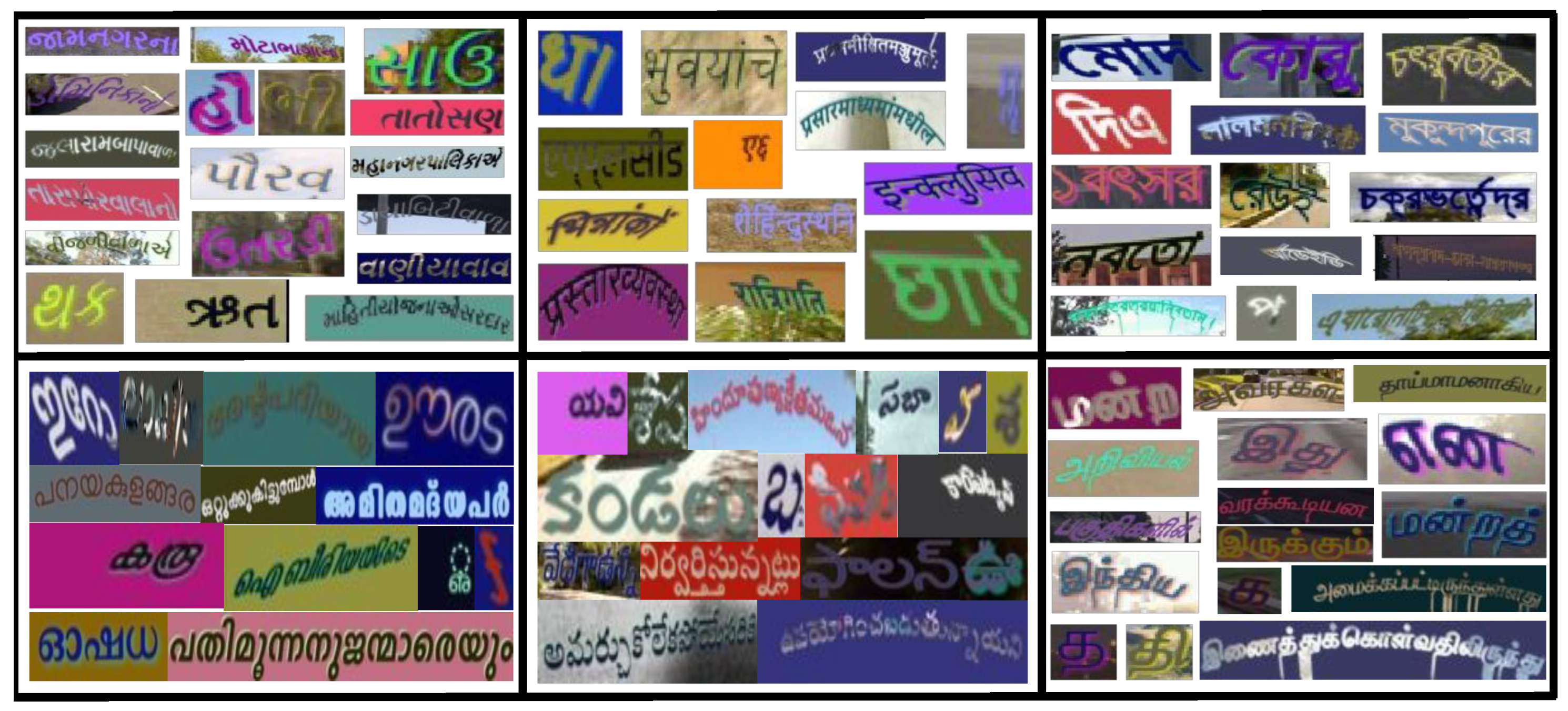
- We also contribute two datasets of around 500 word images in Gujarati and 2535 word images in Tamil from a total of 440 Indian scenes.
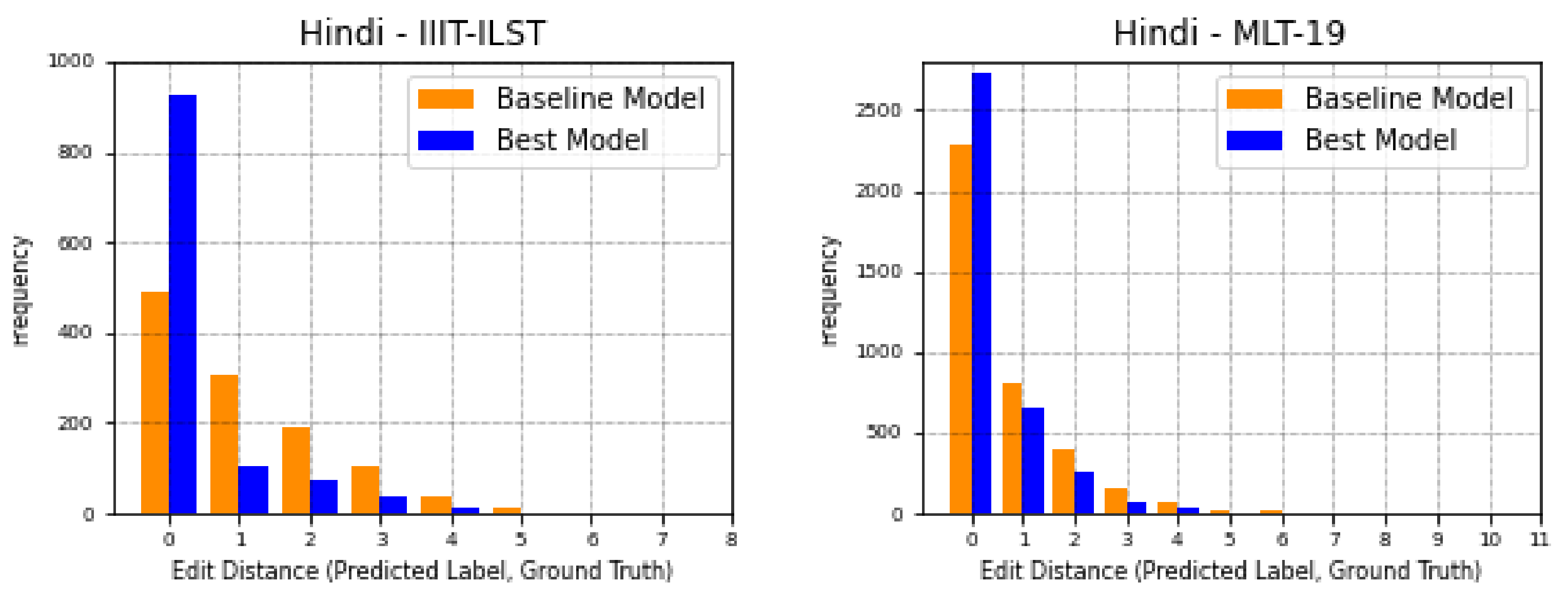
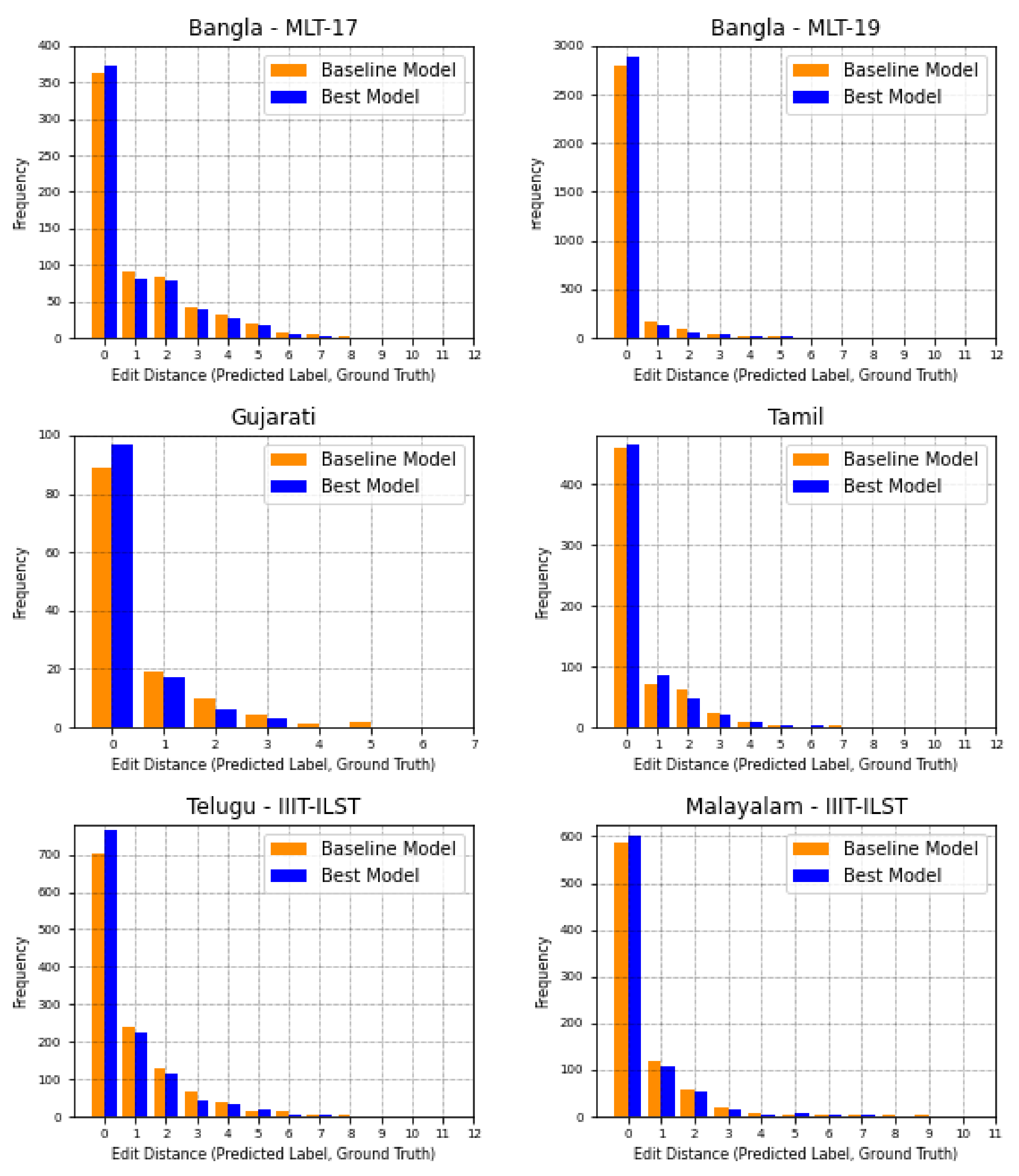
- On IIIT-ILST Hindi, Telugu, and Malayalam datasets, we achieve gains of , , and in Word Recognition Rates (WRRs) over prior works [4,15]. We observe the WRR gains of , , , and over our baseline model on the MLT-19 Hindi and Bangla datasets as well as Gujarati and Tamil datasets we release, respectively. Our model also achieves a notable WRR gain of for the MLT-17 Bangla dataset compared to Bušta et al. [2].
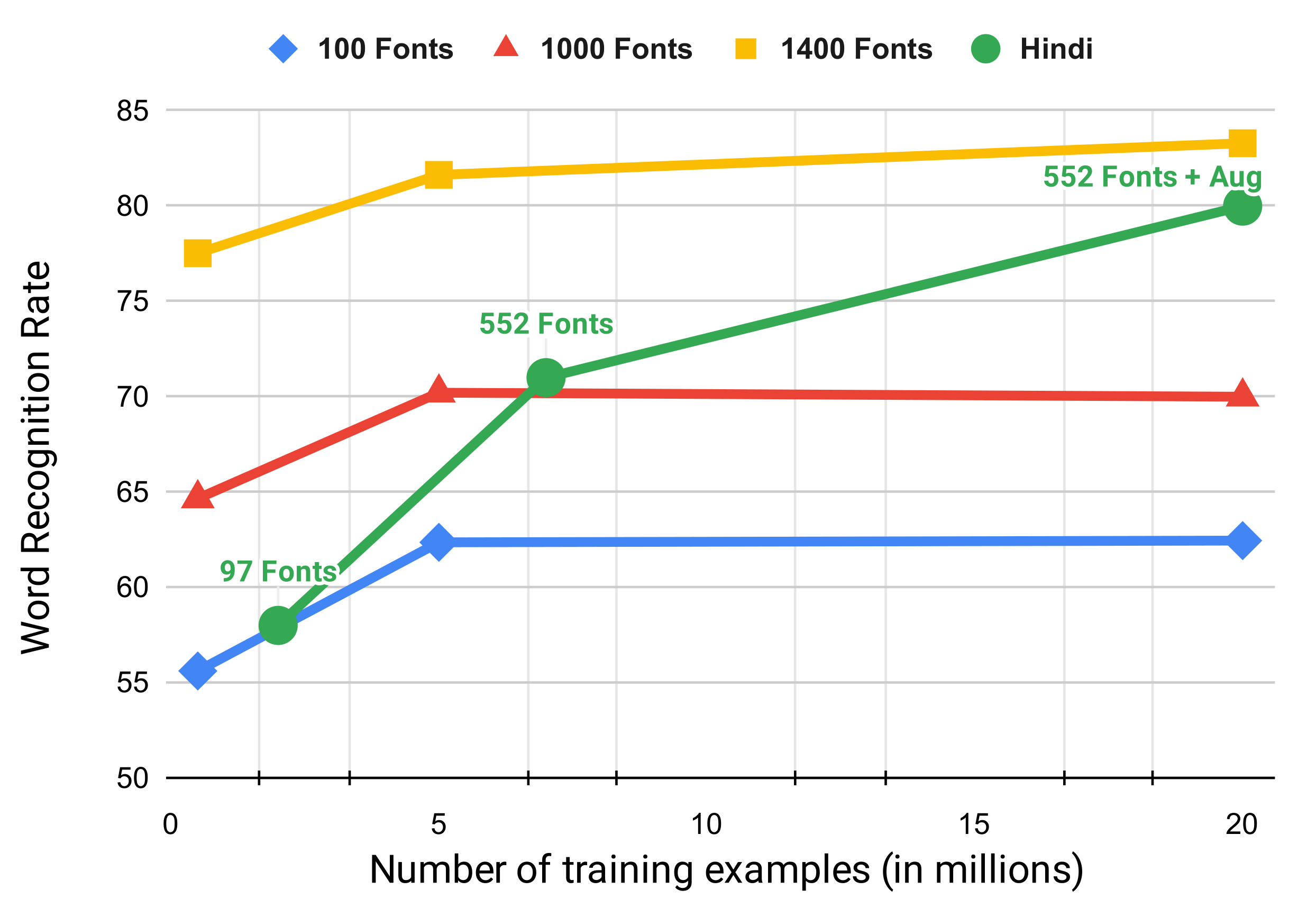
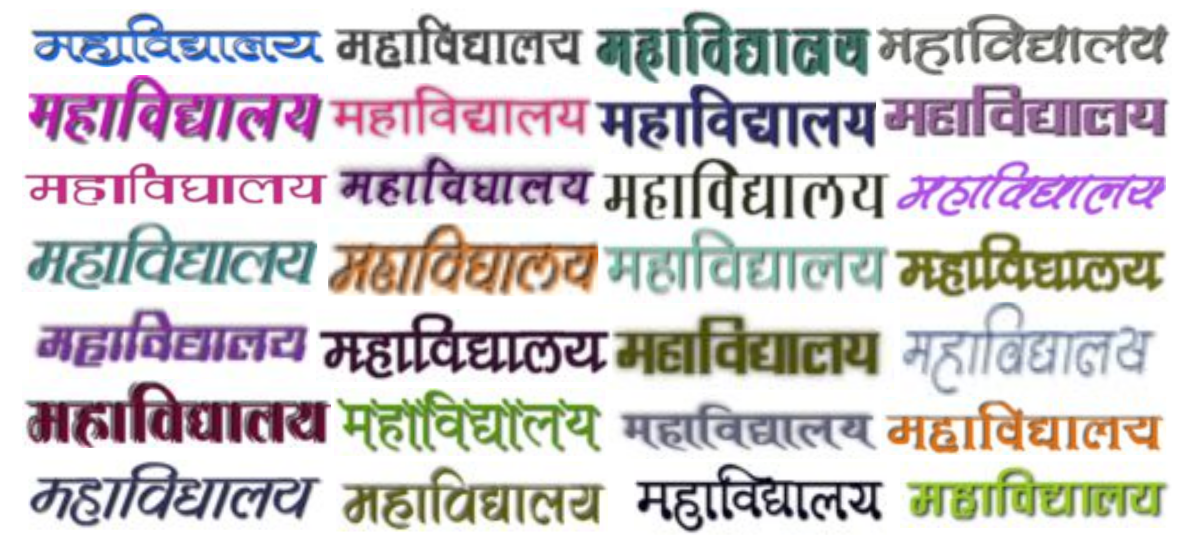
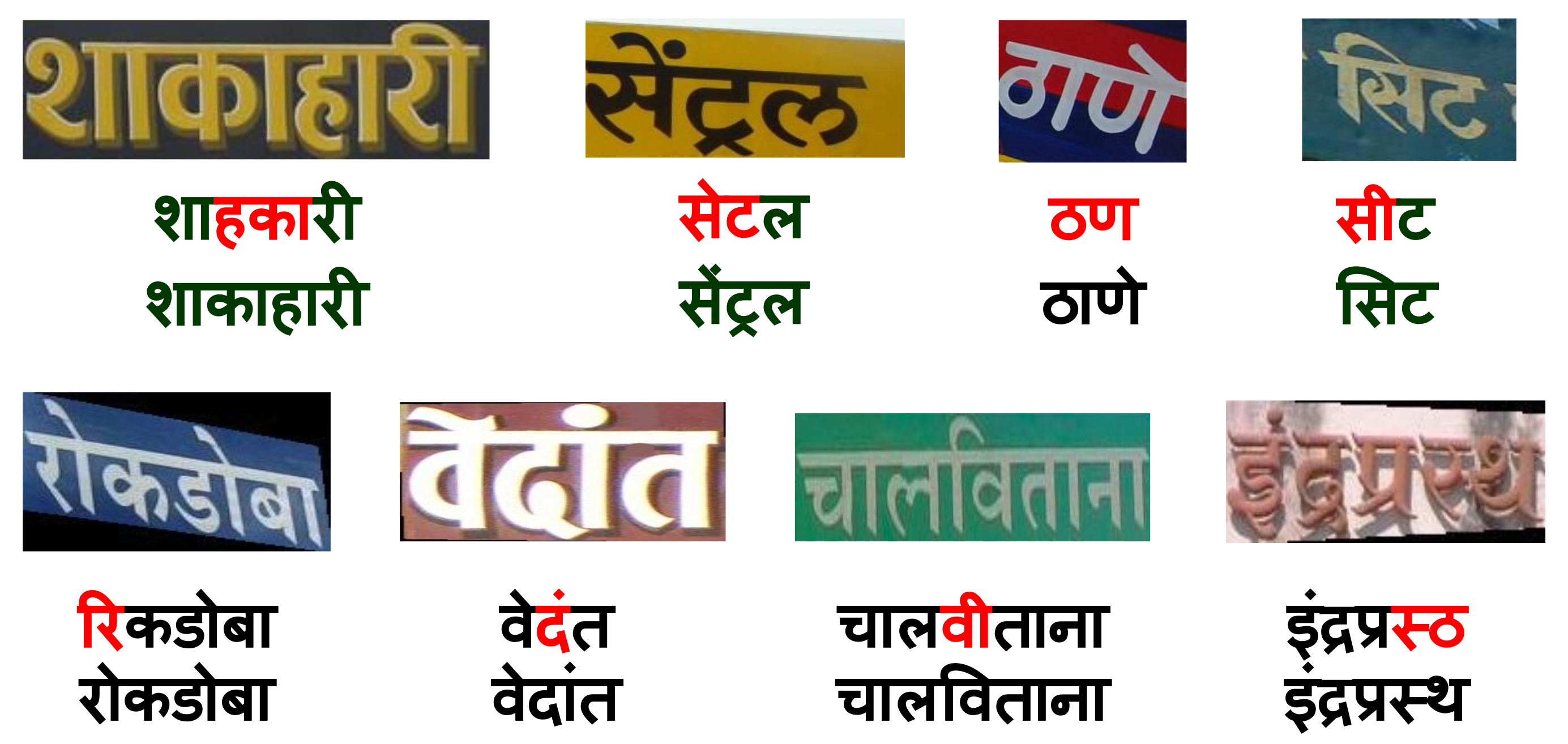
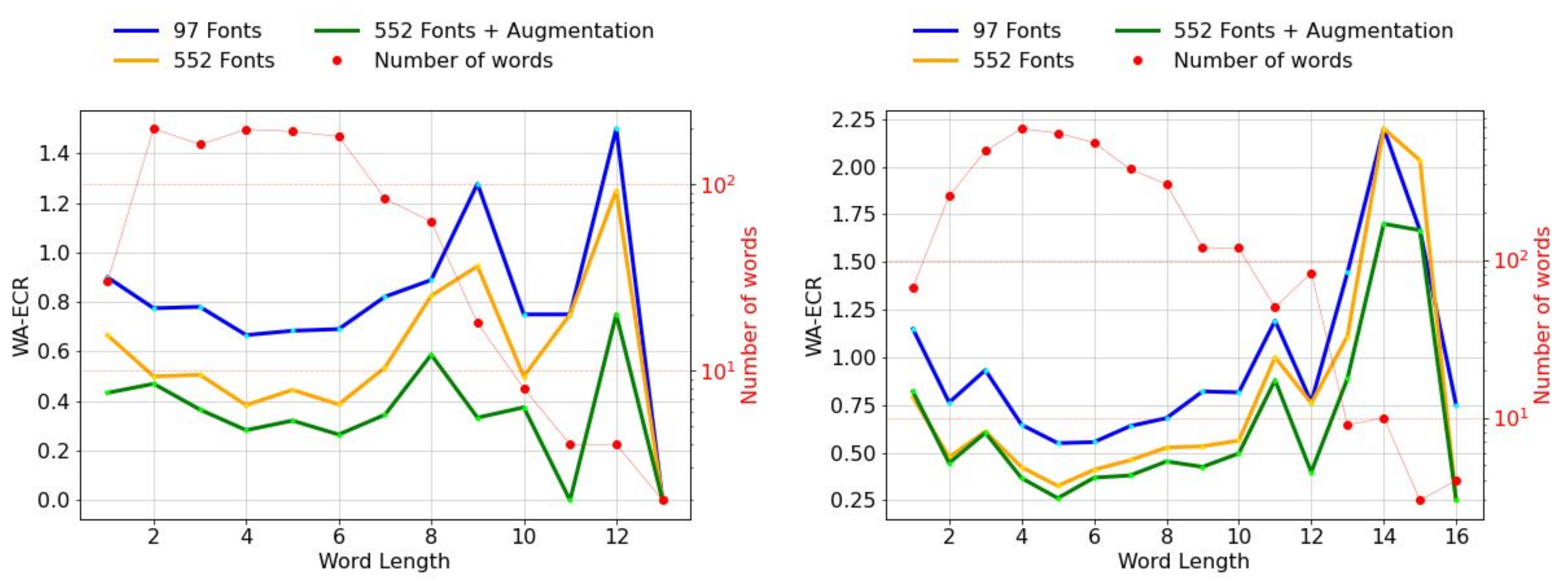
- We are the first to use over 500 Hindi fonts with an existing synthesizer and show that the font diversity can significantly improve non-Latin STR. Specifically, on the IIIT-ILST Hindi dataset, we achieve a remarkable WRR gain of over using more than 500 fonts and different augmentation techniques.
2. Related Work
3. Motivation
4. Datasets
5. Methodology
6. Experiments
7. Results
8. Conclusions
Author Contributions
Funding
Institutional Review Board Statement
Informed Consent Statement
Data Availability Statement
Conflicts of Interest
References
- Lee, C.Y.; Osindero, S. Recursive Recurrent Nets with Attention Modeling for OCR in the Wild. In Proceedings of the IEEE Conference on Computer Vision and Pattern Recognition (CVPR), Las Vegas, NV, USA, 26 June–1 July 2016; pp. 2231–2239. [Google Scholar]
- Bušta, M.; Patel, Y.; Matas, J. E2E-MLT-an Unconstrained End-to-End Method for Multi-Language Scene Text. In Asian Conference on Computer Vision; Springer: Berlin/Heidelberg, Germany, 2018; pp. 127–143. [Google Scholar]
- Huang, Z.; Zhong, Z.; Sun, L.; Huo, Q. Mask R-CNN with Pyramid Attention Network for Scene Text Detection. In Proceedings of the 2019 IEEE Winter Conference on Applications of Computer Vision (WACV), Waikoloa, HI, USA, 7–11 January 2019; pp. 764–772. [Google Scholar]
- Mathew, M.; Jain, M.; Jawahar, C. Benchmarking Scene Text Recognition in Devanagari, Telugu and Malayalam. In Proceedings of the 2017 14th IAPR International Conference on Document Analysis and Recognition (ICDAR), Kyoto, Japan, 9–15 November 2017; Volume 7, pp. 42–46. [Google Scholar]
- Baek, J.; Kim, G.; Lee, J.; Park, S.; Han, D.; Yun, S.; Oh, S.J.; Lee, H. What Is Wrong With Scene Text Recognition Model Comparisons? Dataset and Model Analysis. In Proceedings of the 2019 IEEE/CVF International Conference on Computer Vision (ICCV), Seoul, Korea, 27 October–2 November 2019; pp. 4714–4722. [Google Scholar]
- Yu, D.; Li, X.; Zhang, C.; Han, J.; Liu, J.; Ding, E. Towards Accurate Scene Text Recognition With Semantic Reasoning Networks. In Proceedings of the 2020 IEEE/CVF Conference on Computer Vision and Pattern Recognition (CVPR), Virtual, 14–19 June 2020; pp. 12110–12119. [Google Scholar]
- Hu, W.; Cai, X.; Hou, J.; Yi, S.; Lin, Z. GTC: Guided Training of CTC Towards Efficient and Accurate Scene Text Recognition. In Proceedings of the AAAI Conference on Artificial Intelligence, New York, NY, USA, 7–12 February 2020. [Google Scholar]
- Litman, R.; Anschel, O.; Tsiper, S.; Litman, R.; Mazor, S. SCATTER: Selective Context Attentional Scene Text Recognizer. In Proceedings of the IEEE/CVF Conference on Computer Vision and Pattern Recognition (CVPR), Seattle, WA, USA, 14–19 June 2020. [Google Scholar]
- Qiao, Z.; Zhou, Y.; Yang, D.; Zhou, Y.; Wang, W. SEED: Semantics Enhanced Encoder-Decoder Framework for Scene Text Recognition. In Proceedings of the IEEE/CVF Conference on Computer Vision and Pattern Recognition (CVPR), Virtual, 14–19 June 2020. [Google Scholar]
- Shi, B.; Yang, M.; Wang, X.; Lyu, P.; Yao, C.; Bai, X. ASTER: An Attentional Scene Text Recognizer with Flexible Rectification. IEEE Trans. Pattern Anal. Mach. Intell. 2018, 41, 2035–2048. [Google Scholar] [CrossRef] [PubMed]
- Rehman, A.; Ul-Hasan, A.; Shafait, F. High Performance Urdu and Arabic Video Text Recognition Using Convolutional Recurrent Neural Networks. In Proceedings of the Document Analysis and Recognition—ICDAR 2021 Workshops, Lausanne, Switzerland, 5–10 September 2021. [Google Scholar]
- Nayef, N.; Yin, F.; Bizid, I.; Choi, H.; Feng, Y.; Karatzas, D.; Luo, Z.; Pal, U.; Rigaud, C.; Chazalon, J.; et al. Robust Reading Challenge on Multi-lingual Scene Text Detection and Script Identification—RRC-MLT. In Proceedings of the 14th International Conference on Document Analysis and Recognition (ICDAR), Kyoto, Japan, 9–15 November 2017; Volume 1, pp. 1454–1459. [Google Scholar]
- Nayef, N.; Patel, Y.; Busta, M.; Chowdhury, P.N.; Karatzas, D.; Khlif, W.; Matas, J.; Pal, U.; Burie, J.C.; Liu, C.l.; et al. ICDAR2019 Robust Reading Challenge on Multi-lingual Scene Text Detection and Recognition–RRC-MLT-2019. In Proceedings of the 2019 International Conference on Document Analysis and Recognition (ICDAR), Sydney, NSW, Australia, 20–25 September 2019; pp. 1582–1587. [Google Scholar]
- Gunna, S.; Saluja, R.; Jawahar, C.V. Transfer Learning for Scene Text Recognition in Indian Languages. In Proceedings of the International Conference on Document Analysis and Recognition Workshops, Lausanne, Switzerland, 5–10 September 2021. [Google Scholar]
- Saluja, R.; Maheshwari, A.; Ramakrishnan, G.; Chaudhuri, P.; Carman, M. OCR On-the-Go: Robust End-to-end Systems for Reading License Plates and Street Signs. In Proceedings of the 15th IAPR International Conference on Document Analysis and Recognition (ICDAR), Sydney, NSW, Australia, 20–25 September 2019; pp. 154–159. [Google Scholar]
- Tian, Z.; Huang, W.; He, T.; He, P.; Qiao, Y. Detecting Text in Natural Image with Connectionist Text Proposal Network. In Proceedings of the European Conference on Computer Vision, Amsterdam, The Netherlands, 11–14 October 2016; pp. 56–72. [Google Scholar]
- Zhou, X.; Yao, C.; Wen, H.; Wang, Y.; Zhou, S.; He, W.; Liang, J. EAST: An Efficient and Accurate Scene Text Detector. In Proceedings of the Conference on Computer Vision and Pattern Recognition, Honolulu, HI, USA, 21–26 July 2017; pp. 2642–2651. [Google Scholar]
- Liu, X.; Liang, D.; Yan, S.; Chen, D.; Qiao, Y.; Yan, J. FOTS: Fast Oriented Text Spotting with a Unified Network. In Proceedings of the IEEE Conference on Computer Vision and Pattern Recognition, Salt Lake City, UT, USA, 18–22 June 2018; pp. 5676–5685. [Google Scholar]
- Liao, M.; Shi, B.; Bai, X.; Wang, X.; Liu, W. TextBoxes: A Fast Text Detector with a Single Deep Neural Network. In Proceedings of the Association for the Advancement of Artificial Intelligence, San Francisco, CA, USA, 4–9 February 2017; pp. 4161–4167. [Google Scholar]
- Karatzas, D.; Gomez-Bigorda, L.; Nicolaou, A.; Ghosh, S.; Bagdanov, A.; Iwamura, M.; Matas, J.; Neumann, L.; Chandrasekhar, V.R.; Lu, S.; et al. ICDAR 2015 Competition on Robust Reading. In Proceedings of the 2015 13th International Conference on Document Analysis and Recognition (ICDAR), Tunis, Tunisia, 23–26 August 2015; pp. 1156–1160. [Google Scholar]
- Bušta, M.; Neumann, L.; Matas, J. Deep textspotter: An end-to-end trainable scene text localization and recognition framework. In Proceedings of the International Conference on Computer Vision, Venice, Italy, 22–29 October 2017. [Google Scholar]
- Wang, K.; Babenko, B.; Belongie, S. End-to-End Scene Text Recognition. In Proceedings of the International Conference on Computer Vision, Barcelona, Spain, 6–13 November 2011; pp. 1457–1464. [Google Scholar]
- Shi, B.; Bai, X.; Yao, C. An End-to-End Trainable Neural Network for Image-Based Sequence Recognition and Its Application to Scene Text Recognition. IEEE Trans. Pattern Anal. Mach. Intell. 2016, 39, 2298–2304. [Google Scholar] [CrossRef] [PubMed] [Green Version]
- Liu, W.; Chen, C.; Wong, K.Y.K.; Su, Z.; Han, J. STAR-Net: A SpaTial Attention Residue Network for Scene Text Recognition. In Proceedings of the British Machine Vision Conference, York, UK, 19–22 September 2016; Volume 2. [Google Scholar]
- Zhang, Y.; Gueguen, L.; Zharkov, I.; Zhang, P.; Seifert, K.; Kadlec, B. Uber-Text: A Large-Scale Dataset for Optical Character Recognition from Street-Level Imagery. In Proceedings of the Scene Understanding Workshop-CVPR, Honolulu, Hawaii, USA, 26 July 2017; Volume 2017. [Google Scholar]
- Reddy, S.; Mathew, M.; Gomez, L.; Rusinol, M.; Karatzas, D.; Jawahar, C. RoadText-1K: Text Detection & Recognition Dataset for Driving Videos. In Proceedings of the 2020 IEEE International Conference on Robotics and Automation (ICRA), Paris, France, 31 May–31 August 2020; pp. 11074–11080. [Google Scholar]
- Yu, F.; Xian, W.; Chen, Y.; Liu, F.; Liao, M.; Madhavan, V.; Darrell, T. BDD100K: A Diverse Driving Video Database with Scalable Annotation Tooling. arXiv 2018, arXiv:1805.04687. [Google Scholar]
- Ghosh, M.; Roy, S.; Mukherjee, H.; Sk, O.; Santosh, K.; Roy, K. Understanding movie poster: Transfer-deep learning approach for graphic-rich text recognition. Vis. Comput. 2021. [Google Scholar] [CrossRef]
- Shi, B.; Yao, C.; Liao, M.; Yang, M.; Xu, P.; Cui, L.; Belongie, S.; Lu, S.; Bai, X. ICDAR2017 Competition on Reading Chinese Text in the Wild (RCTW-17). In Proceedings of the 14th International Conference on Document Analysis and Recognition (ICDAR), Kyoto, Japan, 9–15 November 2017; Volume 1, pp. 1429–1434. [Google Scholar]
- Zhang, R.; Zhou, Y.; Jiang, Q.; Song, Q.; Li, N.; Zhou, K.; Wang, L.; Wang, D.; Liao, M.; Yang, M.; et al. ICDAR 2019 Robust Reading Challenge on Reading Chinese Text on Signboard. In Proceedings of the 2019 International Conference on Document Analysis and Recognition (ICDAR), Sydney, NSW, Australia, 20–25 September 2019; pp. 1577–1581. [Google Scholar]
- Yuan, T.; Zhu, Z.; Xu, K.; Li, C.; Mu, T.; Hu, S. A Large Chinese Text Dataset in the Wild. J. Comput. Sci. Technol. 2019, 34, 509–521. [Google Scholar] [CrossRef]
- Sun, Y.; Ni, Z.; Chng, C.K.; Liu, Y.; Luo, C.; Ng, C.C.; Han, J.; Ding, E.; Liu, J.; Karatzas, D.; et al. ICDAR 2019 Competition on Large-Scale Street View Text with Partial Labeling—RRC-LSVT. In Proceedings of the 2019 International Conference on Document Analysis and Recognition (ICDAR), Sydney, NSW, Australia, 20–25 September 2019; pp. 1557–1562. [Google Scholar]
- Tounsi, M.; Moalla, I.; Alimi, A.M.; Lebouregois, F. Arabic Characters Recognition in Natural Scenes using Sparse Coding for Feature Representations. In Proceedings of the 13th International Conference on Document Analysis and Recognition (ICDAR), Tunis, Tunisia, 23–26 August 2015; pp. 1036–1040. [Google Scholar]
- Yousfi, S.; Berrani, S.A.; Garcia, C. ALIF: A Dataset for Arabic Embedded Text Recognition in TV Broadcast. In Proceedings of the 2015 13th International Conference on Document Analysis and Recognition (ICDAR), Tunis, Tunisia, 23–26 August 2015; pp. 1221–1225. [Google Scholar]
- Jung, J.; Lee, S.; Cho, M.S.; Kim, J.H. Touch TT: Scene Text Extractor Using Touchscreen Interface. ETRI J. 2011, 33, 78–88. [Google Scholar] [CrossRef]
- Iwamura, M.; Matsuda, T.; Morimoto, N.; Sato, H.; Ikeda, Y.; Kise, K. Downtown Osaka Scene Text Dataset. In Proceedings of the European Conference on Computer Vision, Amsterdam, The Netherlands, 11–14 October 2016; pp. 440–455. [Google Scholar]
- Singh, A.; Pang, G.; Toh, M.; Huang, J.; Galuba, W.; Hassner, T. TextOCR: Towards Large-Scale End-to-End Reasoning for Arbitrary-Shaped Scene Text. In Proceedings of the IEEE/CVF Conference on Computer Vision and Pattern Recognition (CVPR), Virtual, 19–25 June 2021; pp. 8802–8812. [Google Scholar]
- Ghosh, M.; Mukherjee, H.; Obaidullah, S.M.; Santosh, K.C.; Das, N.; Roy, K. LWSINet: A deep learning-based approach towards video script identification. Multim. Tools Appl. 2021, 80, 29095–29128. [Google Scholar] [CrossRef]
- Ghosh, M.; Roy, S.S.; Mukherjee, H.; Obaidullah, S.M.; Gao, X.Z.; Roy, K. Movie Title Extraction and Script Separation Using Shallow Convolution Neural Network. IEEE Access 2021, 9, 125184–125201. [Google Scholar] [CrossRef]
- Huang, J.; Pang, G.; Kovvuri, R.; Toh, M.; Liang, K.J.; Krishnan, P.; Yin, X.; Hassner, T. A Multiplexed Network for End-to-End, Multilingual OCR. In Proceedings of the IEEE/CVF Conference on Computer Vision and Pattern Recognition (CVPR), Virtual, 19–25 June 2021; pp. 4547–4557. [Google Scholar]
- Ren, S.; He, K.; Girshick, R.; Sun, J. Faster R-CNN: Towards Real-Time Object Detection with Region Proposal Networks. arXiv 2015, arXiv:1506.01497. [Google Scholar] [CrossRef] [PubMed] [Green Version]
- Romera, E.; Alvarez, J.M.; Bergasa, L.M.; Arroyo, R. ERFnet: Efficient Residual Factorized ConvNet for Real-Time Semantic Segmentation. IEEE Trans. Intell. Transp. Syst. 2017, 19, 263–272. [Google Scholar] [CrossRef]
- Russakovsky, O.; Deng, J.; Su, H.; Krause, J.; Satheesh, S.; Ma, S.; Huang, Z.; Karpathy, A.; Khosla, A.; Bernstein, M.; et al. ImageNet Large Scale Visual Recognition Challenge. Int. J. Comput. Vis. 2015, 115, 211–252. [Google Scholar] [CrossRef] [Green Version]
- Vinitha, V.; Jawahar, C. Error Detection in Indic OCRs. In Proceedings of the 2016 12th IAPR Workshop on Document Analysis Systems (DAS), Santorini, Greece, 11–14 April 2016; pp. 180–185. [Google Scholar]
- Gunna, S.; Saluja, R.; Jawahar, C.V. Towards Boosting the Accuracy of Non-Latin Scene Text Recognition. In Proceedings of the 2021 International Conference on Document Analysis and Recognition Workshops (ICDARW), Lausanne, Switzerland, 5–10 September 2021. [Google Scholar]
- Jaderberg, M.; Simonyan, K.; Vedaldi, A.; Zisserman, A. Synthetic Data and Artificial Neural Networks for Natural Scene Text Recognition. In Proceedings of the Workshop on Deep Learning (NIPS), Montreal, QC, Canada, 8–13 December 2014. [Google Scholar]
- Gupta, A.; Vedaldi, A.; Zisserman, A. Synthetic Data for Text Localisation in Natural Images. In Proceedings of the IEEE Conference on Computer Vision and Pattern Recognition, Las Vegas, NV, USA, 26 June–1 July 2016; pp. 2315–2324. [Google Scholar]
- Mishra, A.; Alahari, K.; Jawahar, C.V. Scene Text Recognition using Higher Order Language Priors. In Proceedings of the British Machine Vision Conference, Surrey, UK, 3–7 September 2012. [Google Scholar]
- Zhan, F.; Lu, S.; Xue, C. Verisimilar Image Synthesis for Accurate Detection and Recognition of Texts in Scenes. arXiv 2018, arXiv:abs/1807.03021. [Google Scholar]
- Long, S.; Yao, C. UnrealText: Synthesizing Realistic Scene Text Images from the Unreal World. arXiv 2020, arXiv:abs/2003.10608. [Google Scholar]
- Simonyan, K.; Zisserman, A. Very Deep Convolutional Networks for Large-Scale Image Recognition. arXiv 2014, arXiv:1409.1556. [Google Scholar]
- Szegedy, C.; Ioffe, S.; Vanhoucke, V.; Alemi, A. Inception-v4, Inception-ResNet and the Impact of Residual Connections on Learning. In Proceedings of the AAAI Conference on Artificial Intelligence, San Francisco, CA, USA, 4–9 February 2017; Volume 31. [Google Scholar]
- Zeiler, M. ADADELTA: An adaptive learning rate method. arXiv 2012, arXiv:1212.5701. [Google Scholar]
- Phan, T.Q.; Shivakumara, P.; Tian, S.; Tan, C.L. Recognizing Text with Perspective Distortion in Natural Scenes. In Proceedings of the IEEE International Conference on Computer Vision (ICCV), Sydney, NSW, Australia, 1–8 December 2013. [Google Scholar]
- Burkhard, W.; Keller, R. Some Approaches to Best-Match File Searching. Commun. ACM 1973, 16, 230–236. [Google Scholar] [CrossRef]
- Dwivedi, A.; Saluja, R.; Kiran Sarvadevabhatla, R. An OCR for Classical Indic Documents Containing Arbitrarily Long Words. In Proceedings of the The IEEE/CVF Conference on Computer Vision and Pattern Recognition (CVPR) Workshops, Virtual, 14–19 June 2020. [Google Scholar]


| Language | # Images | Train | Test | , Word Length | # Fonts |
|---|---|---|---|---|---|
| English | 17.5 M | 17 M | 0.5 M | 5.12, 2.99 | >1200 |
| Gujarati | 2.5 M | 2 M | 0.5 M | 5.95, 1.85 | 12 |
| Hindi | 7.5 M | 7 M | 0.5 M | 8.73, 3.10 | 97 |
| Bangla | 2.5 M | 2 M | 0.5 M | 8.48, 2.98 | 68 |
| Tamil | 2.5 M | 2 M | 0.5 M | 10.92, 3.75 | 158 |
| Telugu | 5 M | 5 M | 0.5 M | 9.75, 3.43 | 62 |
| Malayalam | 7.5 M | 7 M | 0.5 M | 12.29, 4.98 | 20 |
| Baseline 1 | Baseline 2 | ||||
|---|---|---|---|---|---|
| S.No. | Language | CRR | WRR | CRR | WRR |
| 1 | English | 77.13 | 38.21 | 86.04 | 57.28 |
| 2 | Gujarati | 94.43 | 81.85 | 97.80 | 91.40 |
| 3 | Hindi | 89.83 | 73.15 | 95.78 | 83.93 |
| 4 | Bangla | 91.54 | 70.76 | 95.52 | 82.79 |
| 5 | Tamil | 82.86 | 48.19 | 95.40 | 79.90 |
| 6 | Telugu | 87.31 | 58.01 | 92.54 | 71.97 |
| 7 | Malayalam | 92.12 | 70.56 | 95.84 | 82.10 |
| Baseline 1 | Baseline 2 | ||||
|---|---|---|---|---|---|
| S.No. | Language | CRR | WRR | CRR | WRR |
| 1 | English → Gujarati | 92.71 (94.43) | 77.06 (81.85) | 97.50 (97.80) | 90.90 (91.40) |
| 2 | English → Hindi | 88.11 (89.83) | 70.12 (73.15) | 94.50 (95.78) | 80.90 (83.93) |
| 3 | Gujarati → Hindi | 91.98 (89.83) | 73.12 (73.15) | 96.12 (95.78) | 84.32 (83.93) |
| 4 | Hindi → Bangla | 91.13 (91.54) | 70.22 (70.76) | 95.66 (95.52) | 82.81 (82.79) |
| 5 | Bangla → Tamil | 81.18 (82.86) | 44.74 (48.19) | 95.95 (95.40) | 81.73 (79.90) |
| 6 | Tamil → Telugu | 87.20 (87.31) | 56.24 (58.01) | 93.25 (92.54) | 74.04 (71.97) |
| 7 | Telugu → Malayalam | 90.62 (92.12) | 65.78 (70.56) | 94.67 (95.84) | 77.97 (82.10) |
| S.No. | Language | Dataset | # Images | Model | CRR | WRR |
|---|---|---|---|---|---|---|
| 1 | Baseline 1 | 84.93 | 72.08 | |||
| 2 | Gujarati | ours | 125 | Baseline 2 | 88.55 | 74.60 |
| 3 | Baseline 2 Eng→Guj | 78.48 | 60.18 | |||
| 4 | Baseline 2 Hin→Guj | 91.13 | 77.61 | |||
| 5 | Mathew et al. [4] | 75.60 | 42.90 | |||
| 6 | Baseline 1 | 78.84 | 46.56 | |||
| 7 | Baseline 2 | 78.72 | 46.60 | |||
| 8 | Hindi | IIIT-ILST | 1150 | Baseline 2 Eng→Hin | 77.43 | 44.81 |
| 9 | Baseline 2 Guj→Hin | 79.12 | 47.79 | |||
| 10 | OCR-on-the-go [15] | - | 51.09 | |||
| 11 | Baseline 2 Guj→Hin FT | 83.64 | 56.77 | |||
| 12 | Baseline 1 | 86.56 | 64.97 | |||
| 13 | Hindi | MLT-19 | 3766 | Baseline 2 | 86.53 | 65.79 |
| 14 | Baseline 2 Guj→Hin | 89.42 | 72.66 | |||
| 15 | Bušta et al. [2] | 68.60 | 34.20 | |||
| 16 | Baseline 1 | 71.16 | 52.74 | |||
| 17 | Bangla | MLT-17 | 673 | Baseline 2 | 71.56 | 55.48 |
| 18 | Baseline 2 Hin→Ban | 72.16 | 57.01 | |||
| 19 | W/t Correction BiLSTM | 83.30 | 58.07 | |||
| 20 | Baseline 1 | 81.93 | 74.26 | |||
| 21 | Bangla | MLT-19 | 3691 | Baseline 2 | 82.80 | 77.48 |
| 22 | Baseline 2 Hin→Ban | 82.91 | 78.02 | |||
| 23 | Baseline 1 | 90.17 | 70.44 | |||
| 24 | Tamil | ours | 634 | Baseline 2 | 89.69 | 71.54 |
| 25 | Baseline 2 Ban→Tam | 89.97 | 72.95 | |||
| 26 | Mathew et al. [4] | 86.20 | 57.20 | |||
| 27 | Telugu | IIIT-ILST | 1211 | Baseline 1 | 81.91 | 58.13 |
| 28 | Baseline 2 | 82.21 | 59.12 | |||
| 29 | Baseline 2 Tam→Tel | 82.39 | 62.13 | |||
| 30 | Mathew et al. [4] | 92.80 | 73.40 | |||
| 31 | Malayalam | IIIT-ILST | 807 | Baseline 1 | 84.12 | 70.36 |
| 32 | Baseline 2 | 91.50 | 72.73 | |||
| 33 | Baseline 2 Tel→Mal | 92.70 | 75.21 |
| S.No. | Dataset | # Synth Images | # Fonts | CRR | WRR |
|---|---|---|---|---|---|
| 1 | IIIT-ILST | 7 M | 97 | 78.72 | 46.60 |
| 2 | 7 M | 552 | 88.00 | 71.45 | |
| 3 | 8 M (Aug) | 552 | 90.92 | 80.33 | |
| 4 | MLT-19 | 7 M | 97 | 86.53 | 65.79 |
| 5 | 7 M | 552 | 87.88 | 67.12 | |
| 6 | 8 M (Aug) | 552 | 90.15 | 72.77 |
| Lexicon-Free | Small (50) | Large (1k) | ||||||
|---|---|---|---|---|---|---|---|---|
| S.No. | Language | Dataset | CRR | WRR | CRR | WRR | CRR | WRR |
| 1 | Gujarati | ours | 91.13 | 77.61 | 100.0 | 100.0 | 92.20 | 78.40 |
| 2 | Hindi | IIIT-ILST | 90.92 | 80.33 | 99.27 | 98.86 | 99.35 | 98.86 |
| 3 | Hindi | MLT-19 | 90.15 | 72.77 | 99.16 | 98.69 | 97.37 | 90.58 |
| 4 | Bangla | MLT-17 | 83.30 | 58.07 | 93.38 | 89.95 | 87.86 | 65.62 |
| 5 | Bangla | MLT-19 | 82.91 | 78.02 | 97.21 | 95.69 | 96.23 | 89.73 |
| 6 | Tamil | ours | 89.97 | 72.95 | 98.03 | 97.00 | 94.40 | 81.70 |
| 7 | Telugu | IIIT-ILST | 86.20 | 62.13 | 96.49 | 94.63 | 89.11 | 63.33 |
| 8 | Malayalam | IIIT-ILST | 92.70 | 75.21 | 98.41 | 97.52 | 93.67 | 76.08 |
Publisher’s Note: MDPI stays neutral with regard to jurisdictional claims in published maps and institutional affiliations. |
© 2022 by the authors. Licensee MDPI, Basel, Switzerland. This article is an open access article distributed under the terms and conditions of the Creative Commons Attribution (CC BY) license (https://creativecommons.org/licenses/by/4.0/).
Share and Cite
Gunna, S.; Saluja, R.; Jawahar, C.V. Improving Scene Text Recognition for Indian Languages with Transfer Learning and Font Diversity. J. Imaging 2022, 8, 86. https://doi.org/10.3390/jimaging8040086
Gunna S, Saluja R, Jawahar CV. Improving Scene Text Recognition for Indian Languages with Transfer Learning and Font Diversity. Journal of Imaging. 2022; 8(4):86. https://doi.org/10.3390/jimaging8040086
Chicago/Turabian StyleGunna, Sanjana, Rohit Saluja, and Cheerakkuzhi Veluthemana Jawahar. 2022. "Improving Scene Text Recognition for Indian Languages with Transfer Learning and Font Diversity" Journal of Imaging 8, no. 4: 86. https://doi.org/10.3390/jimaging8040086
APA StyleGunna, S., Saluja, R., & Jawahar, C. V. (2022). Improving Scene Text Recognition for Indian Languages with Transfer Learning and Font Diversity. Journal of Imaging, 8(4), 86. https://doi.org/10.3390/jimaging8040086