
Fuzzy Color Aura Matrices for Texture Image Segmentation


Abstract
:1. Introduction
1.1. Color Texture Features
1.2. Color Texture Image Segmentation by Pixel Classification
1.3. Fuzzy Color Texture Features
1.4. FCAM for Image Segmentation by Superpixel Classification
2. Superpixel
2.1. Basic SLIC
2.2. Regional SLIC
| Algorithm 1:Regional SLIC. |
| Input: RGB image |
|
| Output: Partition of into superpixels |
3. Fuzzy Color Aura
3.1. Color Aura Set
3.2. Color Aura Set in a Superpixel
3.3. Color Aura Cardinal
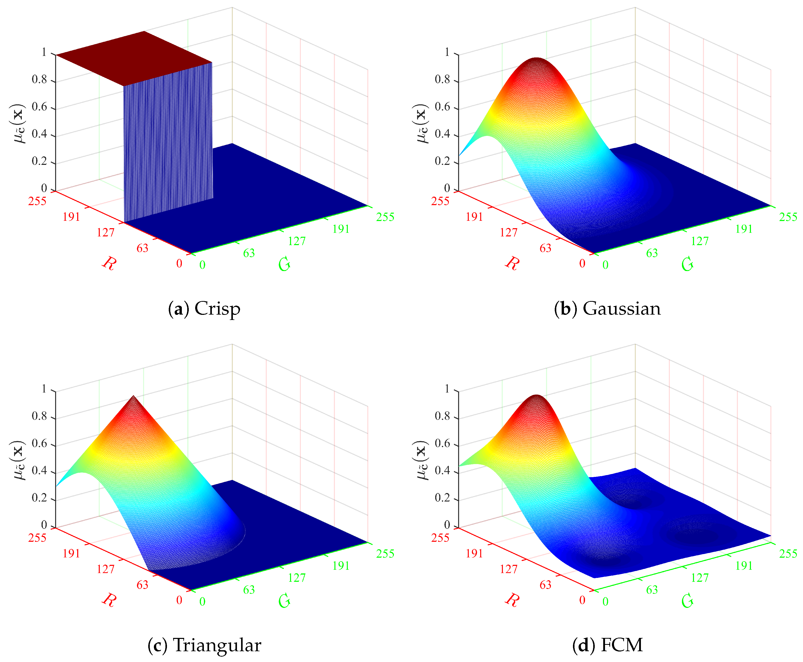
3.4. Fuzzy Color
- the crisp membership function:
- the symmetrical Gaussian function:
- the triangular function:
- or the fuzzy C-means (FCM) membership function:
3.5. Fuzzy Color Aura Set in a Superpixel
3.6. Fuzzy Color Aura Cardinal
4. Experiments
4.1. Experimental Setup
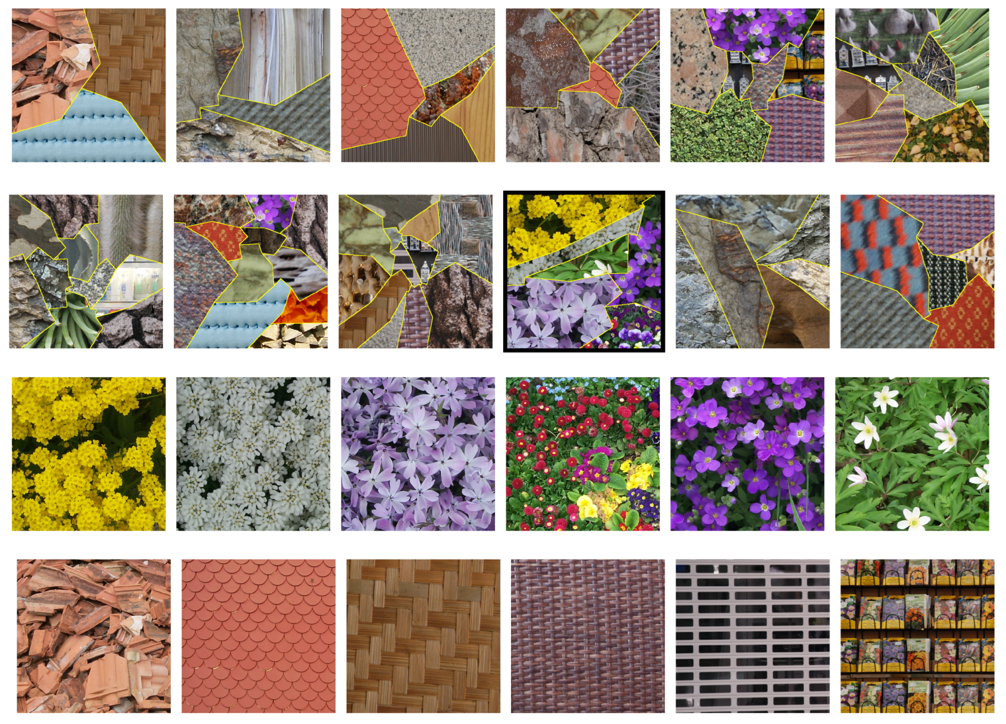
4.1.1. Dataset
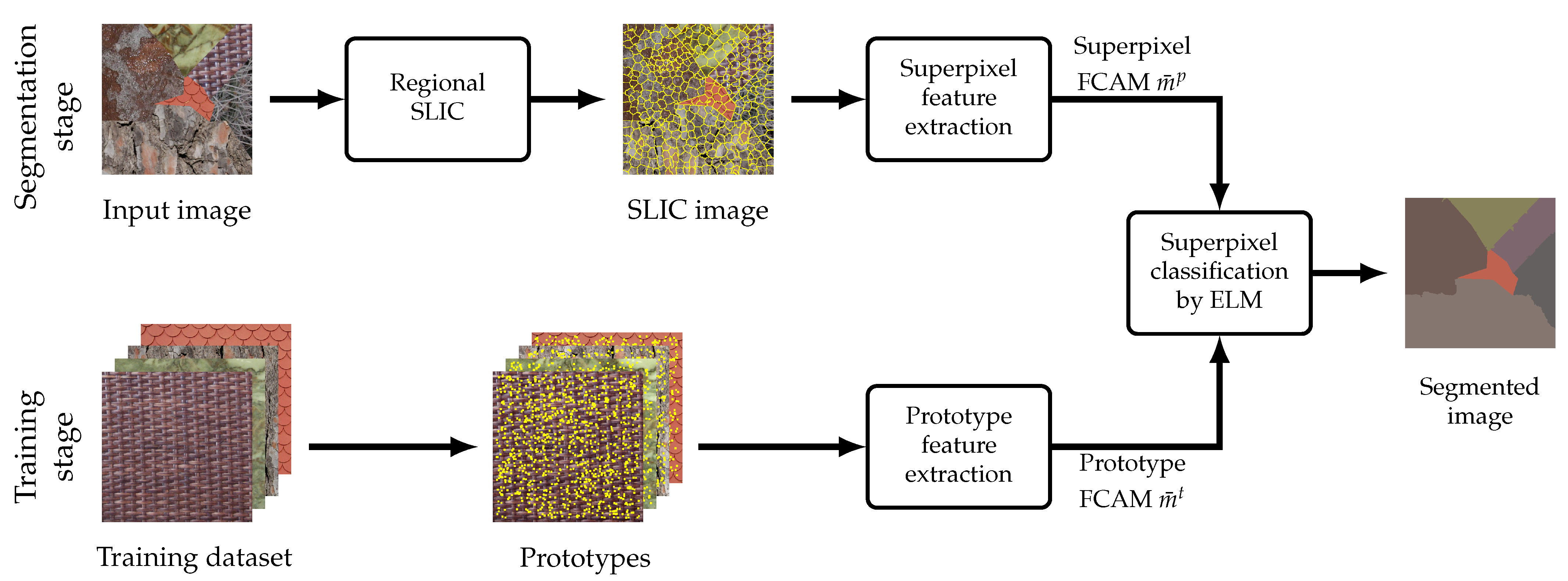
4.1.2. Color Texture Image Segmentation Based on FCAMs
| Algorithm 2:Color texture image segmentation. |
| Input: Test image , training images |
| Parameters: Number T of prototypes per class, number P of superpixels, number C of fuzzy colors, patch half width W, membership function . |
Step 1: Training stage
|
Step 2: Segmentation stage
|
| Step 3: Refinement (optional) |
| Output: Segmented image |
4.1.3. Regional SLIC—Preliminary Assessment
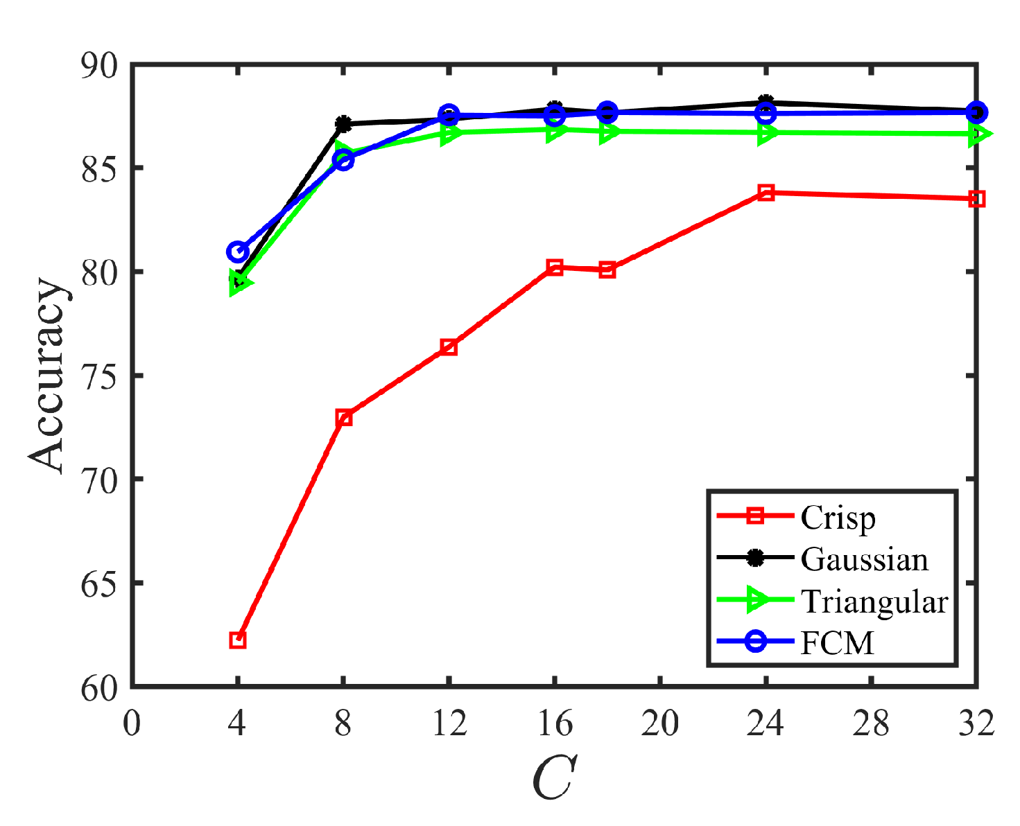
4.1.4. Parameter Settings
4.2. Comparison with Other Fuzzy Texture Features
4.3. Comparison with State-of-the-Art Supervised Segmentation Methods
4.4. Processing Time
5. Conclusions
Author Contributions
Funding
Institutional Review Board Statement
Informed Consent Statement
Data Availability Statement
Conflicts of Interest
References
- Borovec, J.; Švihlík, J.; Kybic, J.; Habart, D. Supervised and unsupervised segmentation using superpixels, model estimation, and graph cut. J. Electron. Imaging 2017, 26, 061610. [Google Scholar] [CrossRef]
- Mikeš, S.; Haindl, M.; Scarpa, G.; Gaetano, R. Benchmarking of remote sensing segmentation methods. IEEE J. Sel. Top. Appl. Earth Obs. Remote Sens. 2015, 8, 2240–2248. [Google Scholar] [CrossRef]
- Akbarizadeh, G.; Rahmani, M. Efficient combination of texture and color features in a new spectral clustering method for PolSAR image segmentation. Natl. Acad. Sci. Lett. 2017, 40, 117–120. [Google Scholar] [CrossRef]
- Zhang, C.; Zou, K.; Pan, Y. A method of apple image segmentation based on color-texture fusion feature and machine learning. Agronomy 2020, 10, 972. [Google Scholar] [CrossRef]
- Ilea, D.E.; Whelan, P.F. Image segmentation based on the integration of colour–texture descriptors–A review. Pattern Recognit. 2011, 44, 2479–2501. [Google Scholar] [CrossRef]
- Haindl, M.; Mikeš, S. A competition in unsupervised color image segmentation. Pattern Recognit. 2016, 57, 136–151. [Google Scholar] [CrossRef]
- Garcia-Lamont, F.; Cervantes, J.; López, A.; Rodriguez, L. Segmentation of images by color features: A survey. Neurocomputing 2018, 292, 1–27. [Google Scholar] [CrossRef]
- Bianconi, F.; Harvey, R.W.; Southam, P.; Fernández, A. Theoretical and experimental comparison of different approaches for color texture classification. J. Electron. Imaging 2011, 20, 043006. [Google Scholar] [CrossRef]
- Ledoux, A.; Losson, O.; Macaire, L. Color local binary patterns: Compact descriptors for texture classification. J. Electron. Imaging 2016, 25, 061404. [Google Scholar] [CrossRef]
- Liu, L.; Chen, J.; Fieguth, P.; Zhao, G.; Chellappa, R.; Pietikäinen, M. From BoW to CNN: Two decades of texture representation for texture classification. Int. J. Comput. Vis. 2019, 127, 74–109. [Google Scholar] [CrossRef] [Green Version]
- Kato, Z.; Pong, T.C.; Lee, J.C.M. Color image segmentation and parameter estimation in a Markovian framework. Pattern Recognit. Lett. 2001, 22, 309–321. [Google Scholar] [CrossRef]
- Nakyoung, O.; Choi, J.; Kim, D.; Kim, C. Supervised classification and segmentation of textured scene images. In Proceedings of the International Conference on Consumer Electronics (ICCE 2015), Las Vegas, NV, USA, 9–12 January 2015; IEEE: Piscataway, NJ, USA, 2015; pp. 473–476. [Google Scholar] [CrossRef]
- Yang, S.; Lv, Y.; Ren, Y.; Yang, L.; Jiao, L. Unsupervised images segmentation via incremental dictionary learning based sparse representation. Inf. Sci. 2014, 269, 48–59. [Google Scholar] [CrossRef]
- Laboreiro, V.R.S.; de Araujo, T.P.; Bessa Maia, J.E. A texture analysis approach to supervised face segmentation. In Proceedings of the IEEE Symposium on Computers and Communications (ISCC 2014), Funchal, Portugal, 23–26 June 2014; IEEE: Piscataway, NJ, USA, 2014; pp. 1–6. [Google Scholar] [CrossRef]
- Panjwani, D.; Healey, G. Markov random field models for unsupervised segmentation of textured color images. IEEE Trans. Pattern Anal. Mach. Intell. 1995, 17, 939–954. [Google Scholar] [CrossRef]
- Chen, K.M.; Chen, S.Y. Color texture segmentation using feature distributions. Pattern Recognit. Lett. 2002, 23, 755–771. [Google Scholar] [CrossRef]
- Salmi, A.; Hammouche, K.; Macaire, L. Constrained feature selection for semisupervised color-texture image segmentation using spectral clustering. J. Electron. Imaging 2021, 30, 013014. [Google Scholar] [CrossRef]
- Jenicka, S. Supervised Texture-Based Segmentation Using Basic Texture Models. In Land Cover Classification of Remotely Sensed Images; Springer: Berlin/Heidelberg, Germany, 2021; pp. 73–88. [Google Scholar]
- Al-Kadi, O.S. Supervised texture segmentation: A comparative study. In Proceedings of the IEEE Jordan Conference on Applied Electrical Engineering and Computing Technologies 2011 (AEECT 2011), Amman, Jordan, 6–8 December 2011; IEEE: Piscataway, NJ, USA, 2011; pp. 1–5. [Google Scholar] [CrossRef]
- Yang, H.Y.; Wang, X.Y.; Wang, Q.Y.; Zhang, X.J. LS-SVM based image segmentation using color and texture information. J. Vis. Commun. Image Represent. 2012, 23, 1095–1112. [Google Scholar] [CrossRef]
- Andrearczyk, V.; Whelan, P.F. Texture segmentation with fully convolutional networks. arXiv 2017, arXiv:1703.05230. [Google Scholar]
- Garcia-Garcia, A.; Orts-Escolano, S.; Oprea, S.; Villena-Martinez, V.; Martinez-Gonzalez, P.; Garcia-Rodriguez, J. A survey on deep learning techniques for image and video semantic segmentation. Appl. Soft Comput. 2018, 70, 41–65. [Google Scholar] [CrossRef]
- Huang, Y.; Zhou, F.; Gilles, J. Empirical curvelet based fully convolutional network for supervised texture image segmentation. Neurocomputing 2019, 349, 31–43. [Google Scholar] [CrossRef]
- Ronneberger, O.; Fischer, P.; Brox, T. U-Net: Convolutional networks for biomedical image segmentation. In Proceedings of the International Conference on Medical Image Computing and Computer-Assisted Intervention (MICCAI 2015), Munich, Germany, 5–9 October 2015; Springer: Cham, Switzerland, 2015; pp. 234–241. [Google Scholar] [CrossRef]
- Wang, W.; Shen, J. Deep visual attention prediction. IEEE Trans. Image Process. 2017, 27, 2368–2378. [Google Scholar] [CrossRef]
- Zhao, H.; Shi, J.; Qi, X.; Wang, X.; Jia, J. Pyramid Scene Parsing Network. In Proceedings of the IEEE Conference on Computer Vision and Pattern Recognition (CVPR 2017), Honolulu, HI, USA, 21–26 July 2017; IEEE: Piscataway, NJ, USA, 2017; pp. 6230–6239. [Google Scholar] [CrossRef]
- Yuan, J.; Wang, D.; Cheriyadat, A.M. Factorization-based texture segmentation. IEEE Trans. Image Process. 2015, 24, 3488–3497. [Google Scholar] [CrossRef] [PubMed]
- Yang, Y.; Han, S.; Wang, T.; Tao, W.; Tai, X.C. Multilayer graph cuts based unsupervised color–texture image segmentation using multivariate mixed Student’s t-distribution and regional credibility merging. Pattern Recognit. 2013, 46, 1101–1124. [Google Scholar] [CrossRef]
- Akbulut, Y.; Guo, Y.; Şengür, A.; Aslan, M. An effective color texture image segmentation algorithm based on hermite transform. Appl. Soft Comput. 2018, 67, 494–504. [Google Scholar] [CrossRef]
- Barcelo, A.; Montseny, E.; Sobrevilla, P. Fuzzy texture unit and fuzzy texture spectrum for texture characterization. Fuzzy Sets Syst. 2007, 158, 239–252. [Google Scholar] [CrossRef]
- Keramidas, E.; Iakovidis, D.; Maroulis, D. Fuzzy binary patterns for uncertainty-aware texture representation. Electron. Lett. Comput. Vis. Image Anal. 2011, 10, 63–78. [Google Scholar] [CrossRef]
- Vieira, R.T.; de Oliveira Chierici, C.E.; Ferraz, C.T.; Gonzaga, A. Local Fuzzy Pattern: A New Way for Micro-pattern Analysis. In Proceedings of the 13th International Conference on Intelligent Data Engineering and Automated Learning (IDEAL 2012), Natal, Brazil, 29–31 August 2012; Lecture Notes in Computer Science. Springer: Cham, Switzerland, 2012; Volume 7435, pp. 602–611. [Google Scholar] [CrossRef]
- Jawahar, C.; Ray, A. Incorporation of gray-level imprecision in representation and processing of digital images. Pattern Recognit. Lett. 1996, 17, 541–546. [Google Scholar] [CrossRef]
- Cheng, H.D.; Chen, C.H.; Chiu, H.H. Image segmentation using fuzzy homogeneity criterion. Inf. Sci. 1997, 98, 237–262. [Google Scholar] [CrossRef]
- Sen, D.; Pal, S.K. Image segmentation using global and local fuzzy statistics. In Proceedings of the IEEE India Council International Conference (INDICON 2006), New Delhi, India, 15–17 September 2006; IEEE: Piscataway, NJ, USA, 2006; pp. 1–6. [Google Scholar] [CrossRef]
- Munklang, Y.; Auephanwiriyakul, S.; Theera-Umpon, N. A novel fuzzy co-occurrence matrix for texture feature extraction. In Proceedings of the 13th International Conference on Computational Science and its Applications (ICCSA 2013), Ho Chi Minh City, Vietnam, 24–27 June 2013; Lecture Notes in Computer Science. Springer: Berlin/Heidelberg, Germany, 2013; Volume 7973, pp. 246–257. [Google Scholar] [CrossRef]
- Khaldi, B.; Kherfi, M.L. Modified integrative color intensity co-occurrence matrix for texture image representation. J. Electron. Imaging 2016, 25, 053007. [Google Scholar] [CrossRef]
- Ledoux, A.; Losson, O.; Macaire, L. Texture classification with fuzzy color co-occurrence matrices. In Proceedings of the IEEE International Conference on Image Processing (ICIP 2015), Québec City, QC, Canada, 27–30 September 2015; IEEE: Piscataway, NJ, USA, 2015; pp. 1429–1433. [Google Scholar] [CrossRef]
- Hammouche, K.; Losson, O.; Macaire, L. Fuzzy aura matrices for texture classification. Pattern Recognit. 2016, 53, 212–228. [Google Scholar] [CrossRef]
- Elfadel, I.M.; Picard, R.W. Gibbs random fields, cooccurrences, and texture modeling. IEEE Trans. Pattern Anal. Mach. Intell. 1994, 16, 24–37. [Google Scholar] [CrossRef]
- Qin, X.; Yang, Y.H. Basic gray level aura matrices: Theory and its application to texture synthesis. In Proceedings of the 10th International Conference on Computer Vision (ICCV’05), Beijing, China, 17–20 October 2005; IEEE: Piscataway, NJ, USA, 2005; Volume 1, pp. 128–135. [Google Scholar] [CrossRef]
- Qin, X.; Yang, Y.H. Aura 3D textures. IEEE Trans. Vis. Comput. Graph. 2007, 13, 379–389. [Google Scholar] [CrossRef]
- Qin, X.; Yang, Y.H. Similarity measure and learning with gray level aura matrices (GLAM) for texture image retrieval. In Proceedings of the IEEE Conference on Computer Vision and Pattern Recognition (CVPR), Washington, DC, USA, 27 June–2 July 2004; IEEE: Piscataway, NJ, USA, 2004; Volume 1, pp. I–326–I–333. [Google Scholar] [CrossRef]
- Wiesmüller, S.; Chandy, D.A. Content based mammogram retrieval using gray level aura matrix. Int. J. Comput. Commun. Inf. Syst. 2010, 2, 217–223. [Google Scholar]
- Liao, S.; Chung, A.C.S. Texture classification by using advanced local binary patterns and spatial distribution of dominant patterns. In Proceedings of the IEEE International Conference on Acoustics, Speech and Signal Processing (ICASSP’07), Honolulu, HI, USA, 15–20 April 2007; IEEE: Piscataway, NJ, USA, 2007; pp. 1221–1224. [Google Scholar] [CrossRef]
- Wang, Y.; Gao, X.; Fu, R.; Jian, Y. Dayside corona aurora classification based on X-gray level aura matrices. In Proceedings of the 9th ACM International Conference on Image and Video Retrieval (CIVR 2010), Xi’an, China, 5–7 July 2010; ACM: New York, NY, USA, 2010; pp. 282–287. [Google Scholar] [CrossRef]
- Hannan, M.A.; Arebey, M.; Begum, R.A.; Basri, H. Gray level aura matrix: An image processing approach for waste bin level detection. In Proceedings of the World Congress on Sustainable Technologies (WCST 2011), London, UK, 7–10 November 2011; IEEE: Piscataway, NJ, USA, 2011; pp. 77–82. [Google Scholar] [CrossRef]
- Khalid, M.; Yusof, R.; Khairuddin, A.S.M. Improved tropical wood species recognition system based on multi-feature extractor and classifier. Int. J. Electr. Comput. Eng. 2011, 5, 1495–1501. [Google Scholar]
- Hannan, M.A.; Arebey, M.; Begum, R.A.; Basri, H. An automated solid waste bin level detection system using a gray level aura matrix. Waste Manag. 2012, 32, 2229–2238. [Google Scholar] [CrossRef]
- Yusof, R.; Khalid, M.; Khairuddin, A.S.M. Application of kernel-genetic algorithm as nonlinear feature selection in tropical wood species recognition system. Comput. Electron. Agric. 2013, 93, 68–77. [Google Scholar] [CrossRef]
- Haliche, Z.; Hammouche, K. The gray level aura matrices for textured image segmentation. Analog. Integr. Circuits Signal Process. 2011, 69, 29–38. [Google Scholar] [CrossRef]
- Haliche, Z.; Hammouche, K.; Postaire, J.G. Texture image segmentation based on the elements of gray level aura matrices. In Proceedings of the Global Summit on Computer & Information Technology (GSCIT 2014), Sousse, Tunisia, 14–16 June 2014; IEEE: Piscataway, NJ, USA, 2014; pp. 1–6. [Google Scholar] [CrossRef]
- Haliche, Z.; Hammouche, K.; Postaire, J.G. A fast algorithm for texture feature extraction from gray level aura matrices. Int. J. Circuits Syst. Signal Process. 2015, 9, 54–61. [Google Scholar]
- Han, J.C.; Zhao, P.; Wang, C.K. Wood species recognition through FGLAM textural and spectral feature fusion. Wood Sci. Technol. 2021, 55, 535–552. [Google Scholar] [CrossRef]
- Achanta, R.; Shaji, A.; Smith, K.; Lucchi, A.; Fua, P.; Süsstrunk, S. SLIC superpixels compared to state-of-the-art superpixel methods. IEEE Trans. Pattern Anal. Mach. Intell. 2012, 34, 2274–2282. [Google Scholar] [CrossRef] [Green Version]
- Chen, X.; Zheng, C.; Yao, H.; Wang, B. Image segmentation using a unified Markov random field model. IET Image Process. 2017, 11, 860–869. [Google Scholar] [CrossRef]
- Mikes, S.; Haindl, M. Texture Segmentation Benchmark. IEEE Trans. Pattern Anal. Mach. Intell. 2021, 44, 5647–5663. [Google Scholar] [CrossRef] [PubMed]
- Huang, G.B.; Zhu, Q.Y.; Siew, C.K. Extreme learning machine: Theory and applications. Neurocomputing 2006, 70, 489–501. [Google Scholar] [CrossRef]
- Liu, M.Y.; Tuzel, O.; Ramalingam, S.; Chellappa, R. Entropy rate superpixel segmentation. In Proceedings of the IEEE Conference on Computer Vision and Pattern Recognition (CVPR’11), Colorado Springs, CO, USA, 20–25 June 2011; IEEE: Piscataway, NJ, USA, 2011; pp. 2097–2104. [Google Scholar] [CrossRef]
- Stutz, D.; Hermans, A.; Leibe, B. Superpixels: An evaluation of the state-of-the-art. Comput. Vis. Image Underst. 2018, 166, 1–27. [Google Scholar] [CrossRef] [Green Version]

 ). and are empty. (c) Superpixels (left) and (right), and aura sets (②) and (
 ). and are empty.
 (c) Superpixels (left) and (right), and aura sets (②) and (). and are empty.
). and are empty.
). and are empty. (c) Superpixels (left) and (right), and aura sets (②) and (). and are empty.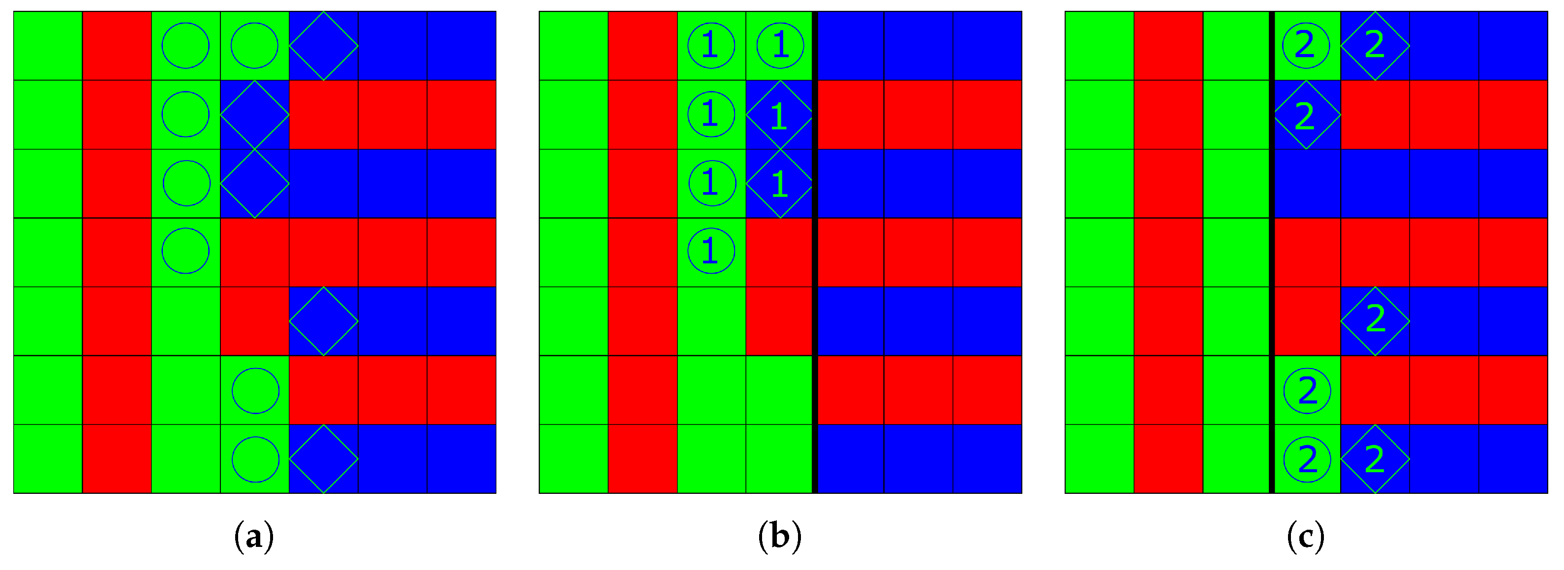


| Metric | ↑BR | ↓UE | ↑ASA | ↑COM |
|---|---|---|---|---|
| Basic SLIC | ||||
| Regional SLIC |
| Feature | Size | Accuracy nr | Accuracy wr | Comp. Time |
|---|---|---|---|---|
| FGLCM | 86.69 | 90.97 | 123.53 | |
| FCCM | 86.52 | 90.77 | 37.62 | |
| FGLAM | 87.24 | 91.28 | 112.32 | |
| FCAM | 87.82 | 92.00 | 33.12 |
| Criteria | MRF | COF | Con- | FCNT | FCNT | EWT- | U-Net | DA | PSP- | FCAM | FCAM |
|---|---|---|---|---|---|---|---|---|---|---|---|
| Col | nr | wr | FCNT | Net | nr | wr | |||||
| ↑ CS | 46.11 | 52.48 | 84.57 | 87.52 | 96.01 | 98.45 | 96.71 | 94.18 | 96.45 | 84.24 | 91.27 |
| ↓ OS | 0.81 | 0.00 | 0.00 | 0.00 | 1.56 | 0.00 | 1.71 | 0.00 | 0.17 | 0.00 | 0.00 |
| ↓ US | 4.18 | 1.94 | 1.70 | 0.00 | 1.20 | 0.00 | 0.00 | 1.18 | 0.41 | 0.00 | 0.00 |
| ↓ ME | 44.82 | 41.55 | 9.50 | 6.70 | 0.78 | 0.37 | 0.68 | 3.42 | 1.23 | 11.45 | 5.93 |
| ↓ NE | 45.29 | 40.97 | 10.22 | 6.90 | 0.89 | 0.46 | 0.48 | 3.24 | 1.12 | 11.39 | 5.36 |
| ↓ O | 14.52 | 20.74 | 7.00 | 7.46 | 2.72 | 0.93 | 0.72 | 3.13 | 2.75 | 4.91 | 2.96 |
| ↓ C | 16.77 | 22.10 | 5.34 | 6.16 | 2.29 | 1.04 | 0.70 | 1.32 | 2.39 | 5.89 | 2.72 |
| ↑ CA | 65.42 | 67.01 | 86.21 | 87.08 | 93.95 | 97.67 | 95.86 | 94.53 | 93.89 | 87.28 | 91.54 |
| ↑ CO | 76.19 | 77.86 | 92.02 | 92.61 | 96.73 | 98.78 | 96.91 | 96.23 | 96.06 | 92.60 | 95.20 |
| ↑ CC | 80.30 | 78.34 | 92.68 | 93.26 | 97.02 | 98.81 | 97.38 | 97.01 | 96.41 | 93.65 | 95.96 |
| ↓ I. | 23.81 | 22.14 | 7.98 | 7.39 | 3.27 | 1.22 | 3.09 | 3.77 | 3.94 | 7.40 | 4.80 |
| ↓ II. | 4.82 | 4.40 | 1.70 | 1.49 | 0.68 | 0.25 | 0.41 | 0.58 | 0.69 | 1.32 | 0.87 |
| ↑ EA | 75.40 | 76.21 | 91.72 | 92.68 | 96.68 | 98.77 | 97.01 | 96.24 | 96.08 | 92.58 | 95.13 |
| ↑ MS | 64.29 | 66.79 | 88.03 | 88.92 | 95.10 | 98.17 | 95.37 | 94.35 | 94.08 | 88.90 | 92.80 |
| ↓ RM | 6.43 | 4.47 | 2.08 | 1.38 | 0.86 | 0.24 | 0.61 | 1.07 | 0.70 | 1.64 | 1.24 |
| ↑ CI | 76.69 | 77.05 | 92.02 | 92.81 | 96.77 | 98.78 | 97.08 | 96.41 | 96.15 | 92.84 | 95.35 |
| ↓ GCE | 25.79 | 23.94 | 11.76 | 12.54 | 5.55 | 2.33 | 2.13 | 3.50 | 4.67 | 11.60 | 7.45 |
| ↓ LCE | 20.68 | 19.69 | 8.61 | 9.94 | 3.75 | 1.68 | 1.46 | 2.47 | 3.52 | 8.76 | 5.31 |
| Image | MRF | COF | Con- | FCNT | EWT- | FCAM | FCAM |
|---|---|---|---|---|---|---|---|
| Col | wr | FCNT | nr | wr | |||
| 01 | 99.79 | 96.19 | 96.92 | 99.12 | 99.91 | 99.54 | 99.72 |
| 02 | 77.36 | 93.02 | 92.70 | 97.71 | 99.51 | 92.66 | 96.79 |
| 03 | 95.60 | 96.56 | 92.33 | 97.47 | 99.21 | 98.66 | 99.03 |
| 04 | 73.20 | 68.63 | 93.73 | 98.41 | 98.77 | 96.38 | 98.58 |
| 05 | 89.72 | 89.67 | 91.64 | 96.64 | 98.95 | 92.95 | 93.83 |
| 06 | 84.00 | 57.59 | 95.78 | 97.30 | 99.52 | 96.97 | 97.64 |
| 07 | 67.74 | 58.08 | 89.71 | 96.09 | 96.71 | 79.65 | 84.70 |
| 08 | 58.12 | 71.27 | 90.10 | 95.67 | 98.80 | 84.16 | 90.21 |
| 09 | 72.95 | 61.29 | 93.23 | 96.70 | 99.35 | 94.90 | 95.47 |
| 10 | 71.52 | 58.97 | 85.72 | 92.52 | 96.69 | 86.36 | 89.51 |
| 11 | 61.28 | 80.88 | 96.82 | 96.72 | 95.32 | 94.44 | 97.12 |
| 12 | 81.55 | 63.01 | 87.20 | 96.03 | 99.51 | 92.74 | 95.84 |
| 13 | 74.35 | 84.32 | 77.02 | 96.10 | 98.48 | 87.99 | 90.11 |
| 14 | 91.29 | 90.32 | 96.51 | 97.75 | 99.17 | 94.25 | 96.39 |
| 15 | 57.77 | 79.61 | 96.26 | 97.70 | 99.56 | 95.31 | 98.61 |
| 16 | 61.33 | 60.63 | 91.19 | 94.31 | 99.46 | 86.23 | 93.92 |
| 17 | 62.74 | 72.31 | 91.92 | 96.96 | 99.38 | 91.21 | 95.10 |
| 18 | 77.81 | 92.96 | 96.16 | 98.24 | 99.58 | 97.18 | 98.54 |
| 19 | 76.07 | 94.98 | 97.02 | 98.55 | 99.78 | 97.64 | 99.39 |
| 20 | 89.68 | 86.87 | 88.48 | 94.66 | 97.91 | 92.82 | 93.44 |
| Average | 76.19 | 77.86 | 92.02 | 96.73 | 98.78 | 92.60 | 95.20 |
| Stage | FCNT | EWT-FCNT | U-Net | DA | PSP-Net | FCAM |
|---|---|---|---|---|---|---|
| Segmentation | 3.61 ms | 1.830 s | 4.98 ms | 3.80 ms | 14.39 ms | 41.14 s |
| Training | - | - | - | - | - | 260.9 s |
Publisher’s Note: MDPI stays neutral with regard to jurisdictional claims in published maps and institutional affiliations. |
© 2022 by the authors. Licensee MDPI, Basel, Switzerland. This article is an open access article distributed under the terms and conditions of the Creative Commons Attribution (CC BY) license (https://creativecommons.org/licenses/by/4.0/).
Share and Cite
Haliche, Z.; Hammouche, K.; Losson, O.; Macaire, L. Fuzzy Color Aura Matrices for Texture Image Segmentation. J. Imaging 2022, 8, 244. https://doi.org/10.3390/jimaging8090244
Haliche Z, Hammouche K, Losson O, Macaire L. Fuzzy Color Aura Matrices for Texture Image Segmentation. Journal of Imaging. 2022; 8(9):244. https://doi.org/10.3390/jimaging8090244
Chicago/Turabian StyleHaliche, Zohra, Kamal Hammouche, Olivier Losson, and Ludovic Macaire. 2022. "Fuzzy Color Aura Matrices for Texture Image Segmentation" Journal of Imaging 8, no. 9: 244. https://doi.org/10.3390/jimaging8090244
APA StyleHaliche, Z., Hammouche, K., Losson, O., & Macaire, L. (2022). Fuzzy Color Aura Matrices for Texture Image Segmentation. Journal of Imaging, 8(9), 244. https://doi.org/10.3390/jimaging8090244