1. Introduction
Monitoring the health of civil engineering infrastructure is crucial to ensure safety and longevity. One of the most important aspects of Structural Health Monitoring (SHM) is the ability to detect, locate, and monitor damage [
1,
2,
3]. The one major damage affecting civil infrastructure safety is a crack. Regular inspection and maintenance of civil infrastructures, such as bridges, pavements, and underground structures, are essential to ensure optimal functioning [
4,
5,
6]. Traditional inspection methods by skilled inspectors have limitations, prompting the need for automated inspections using robotics. This approach offers several benefits, including reduced costs, minimal disruptions, and lower risk [
7,
8,
9,
10].
Automatic defect detection can be separated into two main approaches: white-box and black-box techniques [
11]. The former uses algorithms such as edge detectors and thresholding [
12], whereas the latter employs machine learning and artificial neural networks [
13]. Both methods have unique benefits that depend on the application. Generally, the black box is more effective for initial detection, while the white box is better suited for pixel-by-pixel segmentation [
14].
The VGG deep convolutional neural network architecture, developed by the Visual Geometry Group (VGG), has a well-known success rate in identifying and categorizing cracks in concrete structures [
15]. By incorporating transfer learning and fine-tuning to the VGG architecture, we significantly enhanced detection accuracy, thereby making a valuable contribution to the field of structural health monitoring and image quality assessment.
An adaptive lighting platform integrated with robotics is utilised to capture images of concrete samples in low-light environments to facilitate crack detection. This system features a machine-vision camera fitted with four adjustable arms, each fitted with LED strips [
16]. The images are captured using diffuse lighting. However, using robotics and cameras in low-light environments can introduce potential challenges, such as blur and noise during image capture. These factors can significantly affect the quality of the captured images and affect the model’s recognition capability during the training and testing phases [
17]. So, it is essential to evaluate the quality of these images before feeding them to the image processing algorithms, which can be achieved using a no-reference image quality assessment (NR-IQA) technique called the Blind/Referenceless Image Spatial Quality Evaluator (BRSIQUE) [
18].
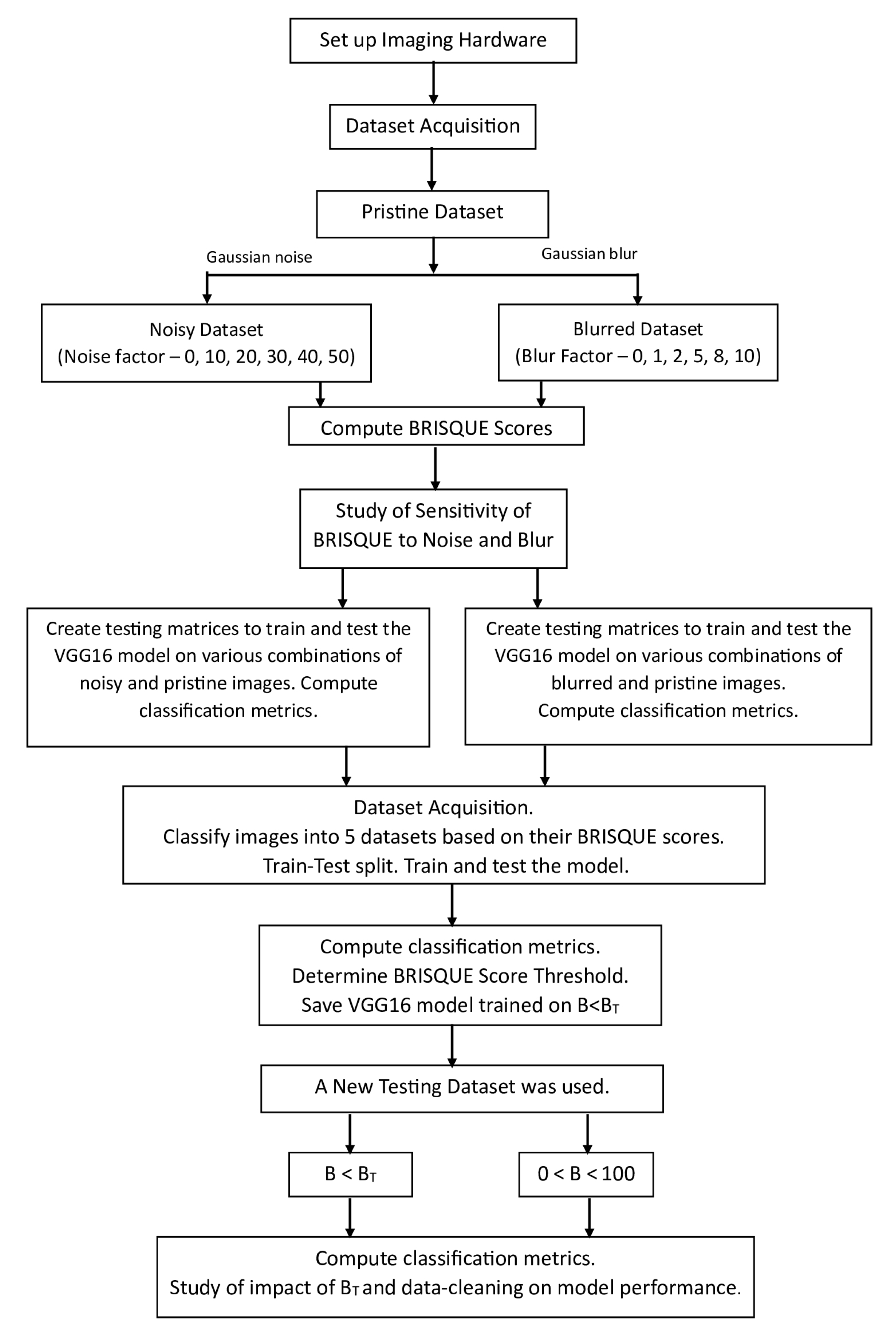
The aim of this study is two-fold. Firstly, it examines the correlation between the BRISQUE image quality metric and the performance of the CNN model in crack detection. The model’s performance will be assessed on pristine images and those with artificially introduced Gaussian noise and Gaussian blur images. The aim is to better understand how image degradation affects crack classification accuracy, F1 score, and Matthew’s correlation coefficient (MCC). Secondly, it proposes a methodology to determine a BRISQUE score threshold (B
) to identify and discard low-quality images from the datasets. Also, the impact of B
and data cleaning on the performance of the model is studied by evaluating the trained threshold-based BRISQUE-assisted deep learning model on an independent testing set. The workflow of the entire process is clearly shown step-by-step in
Figure 1.
2. Background
For major civil and construction assets, semi-autonomous or remote inspections are sometimes carried out with Unmanned Aerial Vehicles (UAVs) or wholesale robotic platforms fit with inspection equipment, as reviewed in [
19]. State-of-the-art research showcases the ability to capture cracked surfaces using moving vehicles [
20] or with UAVs [
21]. In the majority of the reported literature, the process of capturing images is typically conducted separately from the crack detection phase. In an industrial setting, this would mean that any errors or inaccuracies occurring during image capture could not be corrected or adjusted. This would cause either imperfect analysis (requiring error correction) or overlooking significant defects altogether. An innovative system has been employed in our study to capture images of concrete samples in low-light environments, making it easier to identify cracks.
Several factors affect the quality of an image when captured using a camera, including lighting conditions, camera settings, motion blur, lens distortion, and noise. A degraded image refers to a modified version of the original (pristine) image that has been affected by various factors such as blur and noise, either by natural factors or deliberately in post-processing. Since it is uncertain whether a captured image will be natural, noisy, blurry, or distorted in any other way, assigning a score based on the image quality can help in determining the suitability of the image for training or testing the CNN models.
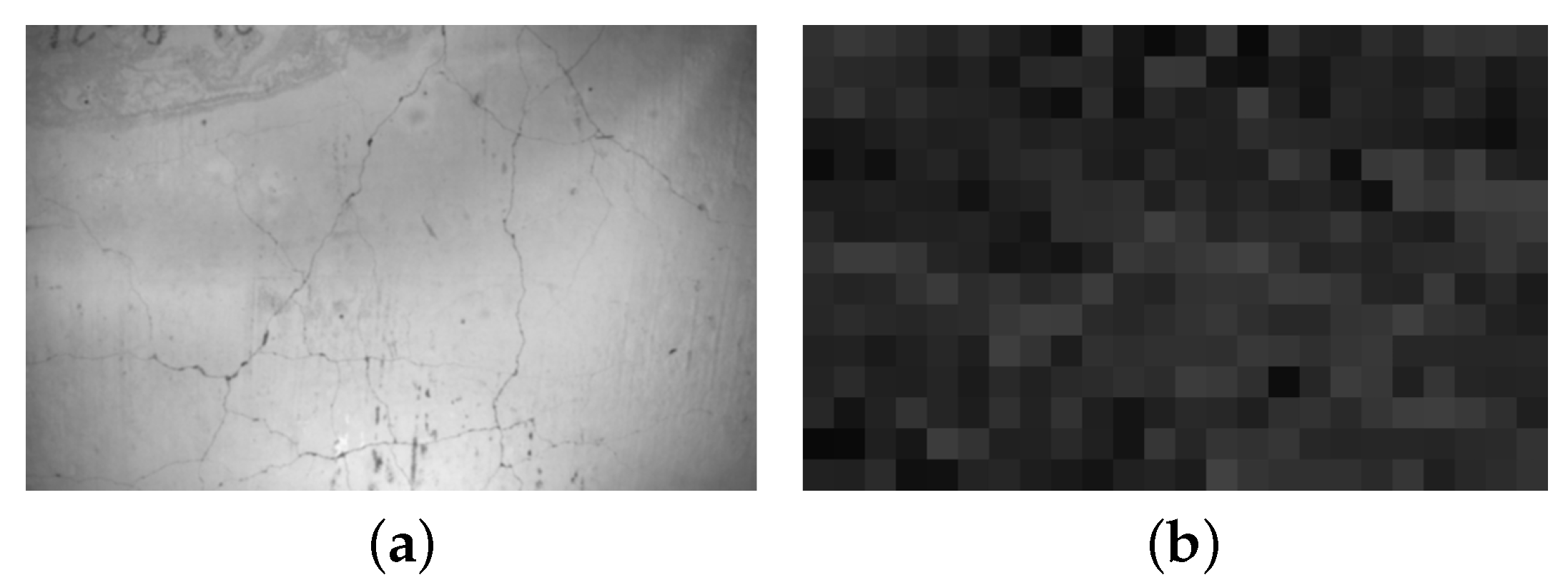
Figure 2 provides an example of a raw image (natural image) and a degraded image (noisy image), along with their BRISQUE scores. Therefore, accurate image quality measurement is essential for developing and evaluating algorithms in various fields. The goal of IQA is to provide methods for measuring image quality in a way that aligns with human perception [
22,
23].
2.1. Image Quality Assessment (IQA)
Image quality assessment is the process of evaluating the quality of an image. It is widely used in machine learning, computer vision, neural physiology, image processing, and other domains where image quality plays an important role [
24]. There are two types of IQA methods.
2.1.1. Subjective Methods
Subjective image quality assessment methods involve gathering individual opinions on the quality of images using a five-level rating scale without participants having full access to the scores or information from others. By averaging the scores provided by the participants, a reference point for image quality is established, and collecting opinions from a larger number of individuals enhances the reliability of these results [
25].
In practical applications, subjective evaluations are often considered the most accurate for assessing image quality. However, they are expensive, time-consuming, and influenced by various factors. To address these issues, objective IQA methods have been developed, which use numerical methods and mathematical models to predict the perceptual quality of the images [
26].
2.1.2. Objective Methods
The development of accurate mathematical models to predict the quality of images similar to human observers has become crucial in objective IQA methods. These models aim to replicate human quality predictions and provide efficient and cost-effective image quality evaluation [
27]. Objective IQA methods extract features from the image and analyse them using a quality score [
28]. IQA research is typically classified into three frameworks: Full-Reference (FR), Reduced-Reference (RR), and No-Reference (NR) or Blind IQA [
29]. FR methods require a reference image, while RR methods use extracted features from the reference image to evaluate image quality. On the other hand, NR methods can assess image quality without the need for a reference image. All three approaches have their advantages, but obtaining the original reference image in real-world applications can be challenging. In such scenarios, using a no-reference metric is more efficient and practical because it does not rely on the availability of the reference image [
30,
31,
32].
2.2. BRISQUE Method
One way to assess the quality of an image is by using no-reference metrics, such as the Blind or No-Reference IQA technique called the Blind or Referenceless Image Spatial Quality Evaluator (BRISQUE). Numerous studies have assessed the effectiveness of BRISQUE techniques in evaluating the quality of medical images [
27] and concrete crack images [
33].
In Ref. [
34], the live road footage captured by a camera mounted on a vehicle was evaluated using the BRISQUE algorithm to determine its quality for road damage detection and driver notification. The quality of raw IRT images and their potential distortions caused by preprocessing were evaluated in [
35] using BRISQUE as a referenceless image quality assessment metric. Ref. [
36] utilised BRISQUE as a no-reference image quality assessment (IQA) technique to evaluate the effectiveness of preprocessing in improving the quality and visibility of low-light images. The focus was on enhancing the visibility for identifying faulty porcelain insulators in a low-voltage power distribution system. Only a limited number of studies have examined the effectiveness of the BRISQUE technique in evaluating the quality of concrete crack images.
BRISQUE employs a support vector regression (SVR) model trained on images with known distortions, such as blur, noise, and artefacts, to compute the image quality score. It compares the distribution of the mean subtracted contrast normalisation (MSCN) of the subject image to the database images. The MSCN of a pixel at location (i, j) is defined by Equation (
1), where I represents the intensity of the pixel,
is the local mean, and
is the local variance in intensity of the surrounding pixels.
The process of identifying image distortions using the BRISQUE model involves generating a histogram of MSCN values. This model can detect various distortions such as blur, noise, and compression by analysing the shape and variance of the distribution. The model then compares these variables to an image database and assigns a score ranging from 1 to 100, with lower scores indicating better image quality. A score close to 0–30 suggests a good (high) image quality, while a score greater than 40 indicates a poor (low) image quality. An example of this is shown in
Figure 2.
This study explores how different types of image degradations, such as Gaussian noise and Gaussian blur, affect the BRISQUE scores. The main goal is to use BRISQUE scores to assess the quality of original and artificially degraded images and determine the stability of neural network models. Additionally, the research seeks to implement a BRISQUE score thresholding technique to discard low-quality images and improve the performance of the image-based crack detection model.
2.3. Convolutional Neural Network (CNN)
CNNs are widely used in computer vision and image classification applications for detecting features and patterns within an image. The VGG architecture, a deep CNN model, has been proven effective in identifying and classifying cracks in concrete structures. The VGG16 model, which has 13 convolutional layers and three fully connected layers, is used in this study as a pre-trained model. This model was originally trained on the ImageNet dataset and can process images that are 224 × 224 pixels with three channels. Its training was based on the ImageNet dataset [
37,
38].
3. Methodology
The primary aim of this research is to assess the image quality by assigning a BRISQUE score to each image captured. Then, a VGG16 neural network model is utilised to train these images to detect cracks on concrete surfaces. This study investigates how well the deep learning models can detect cracks and analyse their relationship with BRISQUE scores. The study also highlights the benefits of using a BRISQUE score threshold (B) to improve the model’s ability to recognise cracks effectively.
3.1. Overview
Our inspection device is built to capture images under diffused lighting conditions, utilizing a machine-vision camera surrounded by four adjustable arms, each fitted with RGB LED strips. These lighting arms are positioned at a 50 degree angle of incidence relative to the concrete surface. An illustration of this setup, using a single arm, is presented in
Figure 3, where D represents working distance, which is explained in subsequent sections.
3.1.1. Image Capture
Engineering standards typically state that crack widths of 0.1 mm to 0.3 mm in concrete structures should be identified for further action [
39]. We have therefore chosen to work towards a minimum spatial resolution of ≤0.1 mm/pixel during image capture.
3.1.2. Hardware and Settings
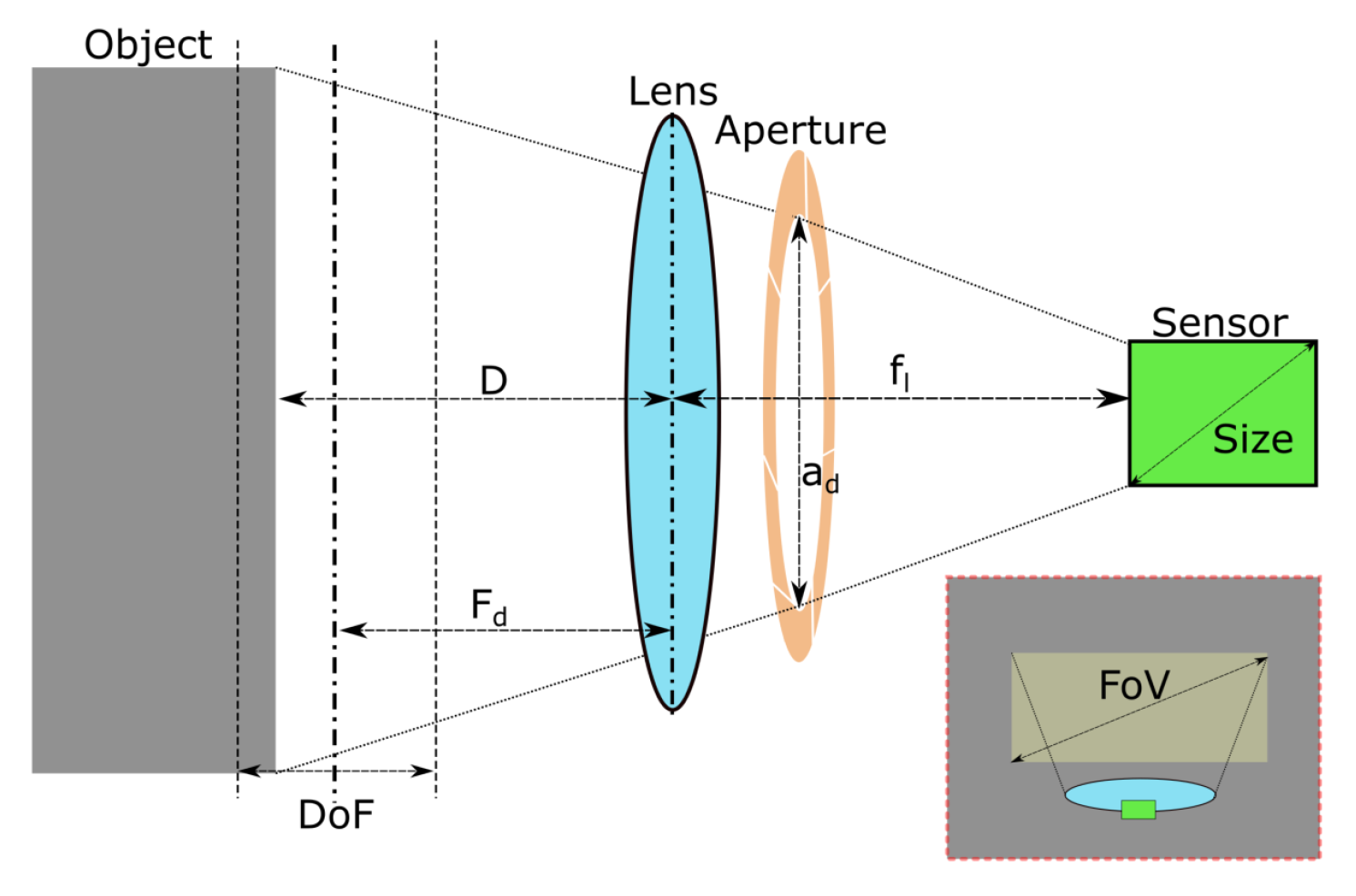
An illustration of the image acquisition hardware is provided in
Figure 4. In this work, a FLIR Blackfly 1” sensor machine vision camera with imaging resolution of 5472 × 3648 pixels were fit with an
= 8 mm focal length lens. Together, these provided a feature resolution of ≤0.1 mm/pixel at a working distance of
D = 350 mm, with a Field of View, FoV, of 574 mm × 383 mm.
The depth of field,
, defines the distances at which objects remain in focus:
where
is the f-number is the ratio of the focal length,
, to aperture diameter,
.
C is the circle of confusion: a subjective limit that defines an acceptable level of loss of focus. It is conventionally calculated by dividing the diagonal size of the camera sensor by 1500.
Equation (
2) shows that high f-numbers result in a high DoF, but this comes with trade-offs, such as a decrease in image capture speed (as image sensor exposure is reduced). Particularly high f-numbers can cause diffraction effects in images, while low f-numbers can cause blurring at image edges. In this work, we selected
= 8 and
= 250 mm. This resulted in no discernible diffraction effects with acceptable levels of edge blurring. This allows objects to be imaged clearly between lens-object distances of 200 mm to 350 mm.
3.2. Dataset Acquisition and Preprocessing
A dataset of high-resolution images of concrete surfaces with visible cracks was obtained for this study. The dataset consisted of damaged, reinforced concrete slabs measuring 500 mm × 500 mm × 10 mm, with crack widths ranging from 0.07 mm to 0.3 mm. The cracks were generated by applying forces at the edges, and the images were captured under diffuse lighting. A preprocessing step was performed to prepare the images for input to the VGG16 model, where the large image shown in
Figure 5 was cropped into blocks of size 224 × 224 pixels.
Overall, a data set of 3600 sub-images, each corresponding to a size of 224 × 224 pixels, was curated. Of this dataset, 2100 images displayed cracks, and 1500 images displayed clear concrete surfaces. The images were manually labelled as cracked or not cracked. The “baseline” images were degraded by introducing common degradations such as Gaussian noise and Gaussian blur. These degradations were chosen as they are commonly produced in real datasets during image acquisition and can severely impact crack classification accuracy.
In this study, we applied Gaussian noise to the original images by increasing the noise level from 10 to 50; an example of this is shown in
Figure 6. In Equation (
3), the coordinates (x,y) represent the pixel coordinates, s(x,y) is the original image, n(x,y) is the added Gaussian noise, and w(x,y) is the resulting noisy image [
40]. The ‘np.random.normal()’ function is used to generate the Gaussian noise.
In this study, we applied Gaussian blur by varying the blur factor from 1 to 10, with the levels being 1, 2, 5, 8, and 10, as represented by Equation (
4), where I is the original image without the blur,
is the blurred image that contains Gaussian blur, G is a Gaussian kernel with standard deviation
, and ⊗ denotes the convolution operation [
41]. Gaussian blur is achieved by convolving the image with a Gaussian kernel using a function called ‘ImageFilter.GaussianBlur()’. A higher blur factor indicates a higher level of blur applied to the image; an example of this is shown in
Figure 7.
3.3. VGG16 CNN Model
In this study, we utilised the VGG16 CNN model trained on ImageNet as a base model shown in
Figure 8. By employing transfer learning, we added layers to the pre-trained model to customise it for our specific task (fine-tuning), enabling the model to learn more efficiently and with fewer training examples [
42,
43,
44,
45].
To perform binary classification of concrete images, we utilized transfer learning and loaded a pre-trained VGG16 model that has been previously trained on a large ImageNet dataset. By leveraging the learned features from the VGG16 model, we can save time and resources by avoiding the need for extensive training on our specific dataset. To fine-tune the model, we strategically decided to freeze all the layers except the last six layers of the base model. Our approach, which combined transfer learning, selective fine-tuning, and specialized classification layers, played a pivotal role in achieving state-of-the-art results in our research.
We used the Adam optimiser [
46] with binary cross-entropy loss and accuracy metrics to compile the new model. The model was trained for 10 epochs, with a batch size of 32, and then evaluated on the testing data. Dropout was applied in the network architecture to prevent overfitting, and a dense layer with sigmoid activation was employed for binary classification. The performance of the model was assessed by computing the confusion matrix and performance metrics. The VGG16 model implemented in this study is trained and tested on pristine, noisy, and blurred images.
3.4. Performance Metrics
We used separate training and testing datasets to evaluate the performance of the VGG16 model on the baseline, noisy, and blurred datasets. The model was trained on the training dataset and was used to generate predictions on the testing dataset. We then converted the predicted probabilities to binary class labels using a threshold of 0.5. The performance of the model was assessed using a confusion matrix generated by comparing the predicted labels to the actual labels of the testing dataset. The confusion matrix provided information about correctly and incorrectly classified instances, represented by true positive (TP), true negative (TN), false positive (FP), and false negative (FN) values. Finally, these values range from 0 to 1, with 1 indicating good and 0 indicating bad, and are utilised to calculate various evaluation metrics as shown in
Table 1 [
47].
3.5. Testing Matrix Analysis
A testing matrix was created to evaluate the performance of the VGG16 model under different conditions. This matrix outlines the different combinations of training and testing scenarios used during the evaluation, as listed in
Table 2. The rows indicate the testing conditions, which include noisy, blurred, and pristine images, while the columns represent the training conditions, including noisy, blurred, and pristine images. The “x” marks in the matrix indicate specific training and testing combinations. For example, “Train on Noisy, Test on Noisy” means that the model was trained on noisy images and then tested on noisy images. Similarly, “Train on Blur, Test on Pristine” means that the model was trained on blur images and then tested on pristine images. Thus, the testing matrix provides valuable insights into the crack detection model’s performance under different training and testing combinations.
4. Results
The impact of image degradation on image quality can significantly affect a model’s recognition capabilities. Therefore, it is vital to assess image quality using metrics that are sensitive to various types of image degradations. In this section, we evaluate the sensitivity of the BRISQUE image quality metric to different types of degraded images.
4.1. The Sensitivity of BRISQUE to Noise and Blur
In this study, we examined the effect of noise and blur on image quality by analysing the BRISQUE scores and utilising colour maps. Colour maps help to visually evaluate the image quality based on colour intensity.
Figure 5a represents the baseline (pristine/original) image and its corresponding colour map of BRISQUE scores, which is plotted after data preprocessing, explained in
Section 3.2. As shown in
Figure 5b, lighter pixels in the colour map indicate lower BRISQUE scores, indicating better image quality. On the other hand, darker pixels represent higher BRISQUE scores, indicating degraded image quality. Different types of degraded images were analysed to determine their effects on BRISQUE.
We investigated the relationship more deeply by introducing various levels of noise and blur to the original images.
Figure 6 and
Figure 7 display the images with noise level 50 and blur level 8, respectively, along with their corresponding colour maps of BRSIQUE scores. The colour maps clearly show that regions with greater noise or blur have darker pixels, indicating lower image quality and higher BRISQUE scores.
Figure 9 displays the BRISQUE scores for different levels of noise and blur. The left subplot illustrates the BRISQUE scores for noise levels ranging from 0 to 50, while the right subplot illustrates the BRISQUE scores for blur levels ranging from 0 to 10. Both subplots feature a normal line representing the training data and a dashed line representing the testing data. As we can see from this plot, the BRISQUE score increases as the noise and blur levels increase, indicating a decline in image quality.
Studying the colour maps and their corresponding BRSIQUE scores provides valuable insights into analysing the impact of noise and blur on image quality. Through these images, it becomes evident that the baseline image has the lowest score. As noise and blur levels increase, the BRSIQUE score rapidly increases, indicating a decline in image quality. Therefore, assessing the quality of the images is imperative, as it significantly impacts the model recognition capabilities discussed in subsequent sections.
4.2. Summary of Classification Metrics on Noisy Images
The VGG16 neural network model was analysed on various datasets using three widely used evaluation metrics, namely accuracy, F1 score, and Matthew’s correlation coefficient. The model underwent training and testing on both original (pristine) datasets and datasets with varying noise levels, as shown in
Figure 10 and
Table 3. The testing matrix utilised ‘x’ marks to denote different training and testing dataset combinations used to evaluate the model’s performance.
“Train on Pristine, Test on Pristine” signifies that the model was trained and tested on pristine images, i.e., clear images;
“Train on Pristine, Test on Noisy” signifies that the model was trained using pristine images and then tested on images with varying noise levels;
“Train on Noisy, Test on Noisy” signifies that the model was trained and tested on images with varying noise levels.
The graph in
Figure 10 shows that the X-axis represents various datasets, as listed in
Table 3. These datasets were used to train and test the VGG16 model. The bar graph above, labelled “Train on Pristine and Test on Noisy”, indicates that the model was trained on a clean dataset and then tested on six datasets with increasing noise levels, ranging from 0% to 50%. On the other hand, the bar graph below, labelled “Train and Test on Noisy”, shows that the model was trained and tested on datasets with increasing noise levels, ranging from 0% to 50%. In this case, 0% noisy dataset constitutes pristine (original) and clear images. The Y-axis of the graph represents the performance of each model, as measured by three metrics—accuracy, F1 score, and MCC. The black bars represent accuracy, the dark grey bars represent the F1 score, and the light grey bars represent MCC.
Based on the data presented in the graph, it can be observed that the performance of the VGG16 model declines with an increase in the level of noise in the dataset for all three metrics. Statistical analysis of the data were conducted using a one-way analysis of variance (ANOVA) [
48], which yielded a
p-value of 2.92 × 10
. This low p-value indicates that the results are statistically significant and that the null hypothesis can be rejected. Thus, there is strong evidence to support the alternate hypothesis, which suggests a significant difference between the compared groups. The model was initially trained and tested on the clean, original dataset, and it achieved the highest scores across all three metrics. However, as the level of noise in the dataset increased, the performance of the VGG16 model dropped significantly, with the models trained on the 40% and 50% noisy datasets performing the worst. Regarding the metrics, both the accuracy and F1 score exhibited similar trends, with performance gradually declining as the noise level increased. On the other hand, the MCC demonstrated a more noticeable performance drop as the noise level increased.
Based on the findings, it appears that the VGG16 model is quite sensitive to noise in the dataset. The model’s performance may significantly decrease when the noise level increases. In addition, looking at
Figure 9 and examining the BRISQUE scores of pristine and degraded images with varying noise levels, it becomes clear that even a moderate increase in noise levels can lead to significantly higher BRSIQUE scores, indicating lower image quality. Therefore, training and testing deep learning models on high-quality images (lower BRISQUE scores) is always better to ensure accurate crack detection and classification. By comparing the performance of the model on different datasets, we can gain insights into the suitability of the model for real-world scenarios where image quality cannot be guaranteed.
4.3. Summary of Classification Metrics on Blurred Images
The VGG16 neural network model was analysed on various datasets using three widely used evaluation metrics, namely accuracy, F1 score, and Matthew’s correlation coefficient. The model underwent training and testing on both original (pristine) datasets and datasets with varying blur levels, as shown in
Figure 11 and
Table 4. The testing matrix utilised ‘x’ marks to denote different training and testing dataset combinations used to evaluate the model’s performance.
“Train on Pristine, Test on Pristine” signifies that the model was trained and tested on pristine images, i.e., clear images;
“Train on Pristine, Test on Blur” signifies that the model was trained using pristine images and then tested on images with varying levels of blur;
“Train on Blur, Test on Blur” signifies that the model was trained and tested on images with varying levels of blur.
In
Figure 11, the X-axis represents the datasets listed in
Table 4, which are used for training and testing the VGG16 model. The bar graph above, labelled “Train on Pristine and Test on Blur”, indicates that the model was trained on a pristine dataset but then tested on five distinct datasets with varying levels of blur, ranging from 0% to 10%., and the bar graph below, “Train and Test on Blur” shows that the model was trained and tested on datasets with increasing levels of blur, from 0% to 10%, where 0% blurred dataset represents pristine (original) and clear images. The Y-axis shows the performance of each model, as measured by the three metrics: accuracy, F1 score, and MCC. The black bars represent accuracy, the dark grey bars represent the F1 score, and the light grey bars represent MCC.
Based on the graph, it can be observed that the model’s performance declines in correlation with the increase in the percentage of blur present within the dataset. After conducting a one-way ANOVA on the data, a p-value of 0.0028 was obtained from the statistical analysis. This p-value is considerably low, indicating that the outcome is statistically significant, leading to the rejection of the null hypothesis. This strong evidence supports the alternative hypothesis, which means that the results are statistically significant.
When the model was trained and tested on a pristine dataset without blurring, it achieved the highest scores for all three metrics. However, as the level of blur increased, the model’s accuracy, F1 score, and MCC decreased. For some, F1 and MCC scores were represented as zero in
Figure 11, suggesting no true positives were identified in the predictions. This could be due to the model’s inability to correctly classify any images in the testing set, indicating overfitting and poor performance on that dataset.
As shown in
Figure 11, the VGG16 model is highly sensitive to blur in the dataset, and its performance may decrease significantly when the blur level is high. This highlights the importance of careful data pre-processing in deep learning applications. Moreover,
Figure 9 shows that higher blur levels result in higher BRISQUE scores, indicating lower image quality. This highlights the need to reduce blur in images or remove blurred images before using them in deep learning models. This analysis aimed to assess the suitability of the VGG16 model for real-world scenarios where images may be blurred due to motion or defocus. It underscores the importance of thorough data preparation and cleaning in deep learning applications to ensure high-quality data and optimal model performance.
4.4. Optimizing BRISQUE Score Threshold for Crack Detection
This study aimed to determine a BRISQUE score threshold (B
) that could be used to identify and discard images with excessive degradation during preprocessing to improve the performance of the crack detection model. The study utilised a dataset comprising 5665 images. The images were classified into five datasets based on their BRISQUE scores as shown in
Table 5. Additionally, each set was divided into train and test sets, and they were manually labelled as either positive (cracks) or negative (no cracks). The VGG16 model was then trained and tested on each dataset, and various metrics were calculated to evaluate its performance.
The performance of the VGG16 neural network model for crack detection and classification was evaluated using different BRISQUE score thresholds ranging from <45 to <85, as shown in
Table 5. The analysis revealed that the model’s optimal performance was achieved when the BRISQUE score threshold was set to <45, despite the limited availability of training images. However, the model’s performance gradually decreased as the BRISQUE score threshold increased from <55 to <85. This decrease was not consistently linear due to variations in the number of training images used.
In general, we know that the performance of a model is positively correlated with the number of training images. In particular, increasing the training set size from 720 to 2160 images has improved model performance for BRISQUE score thresholds <55 and <65. However, it should be noted that this positive correlation does not always hold. The performance of the model decreased when the dataset included images with BRISQUE scores <75 and <85. Interestingly, despite having fewer training images, the model achieved its best performance when the BRISQUE score threshold was set to <45. This highlights the importance of image quality in determining neural network performance.
The distribution of BRISQUE scores is visually represented in
Figure 12, which shows distinct score intervals created using histogram binning. The model was trained and tested on images with BRISQUE scores threshold <45 and achieved an accuracy of 0.8, an F1 score of 0.77, and an MCC of 0.606. However, as the BRISQUE score threshold increased, the effectiveness of the model decreased. This implies that the quality of the image greatly influences the accuracy of the crack detection model. It was observed when the threshold of the BRISQUE score was set to <85; the model achieved an accuracy of 0.61, an F1 score of 0.69, and an MCC of 0.30. Hence, images with high levels of degradation can significantly degrade the model’s performance and should be discarded. To summarise, every model has a certain threshold for low-quality images, at which they fail to detect cracks on concrete surfaces. Therefore, allowing only images with BRISQUE scores less than the threshold value helps to improve the crack detection performance. In conclusion, image quality significantly influences the performance of the neural network model for crack detection and classification. The model achieves optimal results when trained on high-quality images, leading to faster training and testing times and lower computational costs by avoiding unnecessary processing of low-quality images.
4.5. BRISQUE-Based Data Cleaning
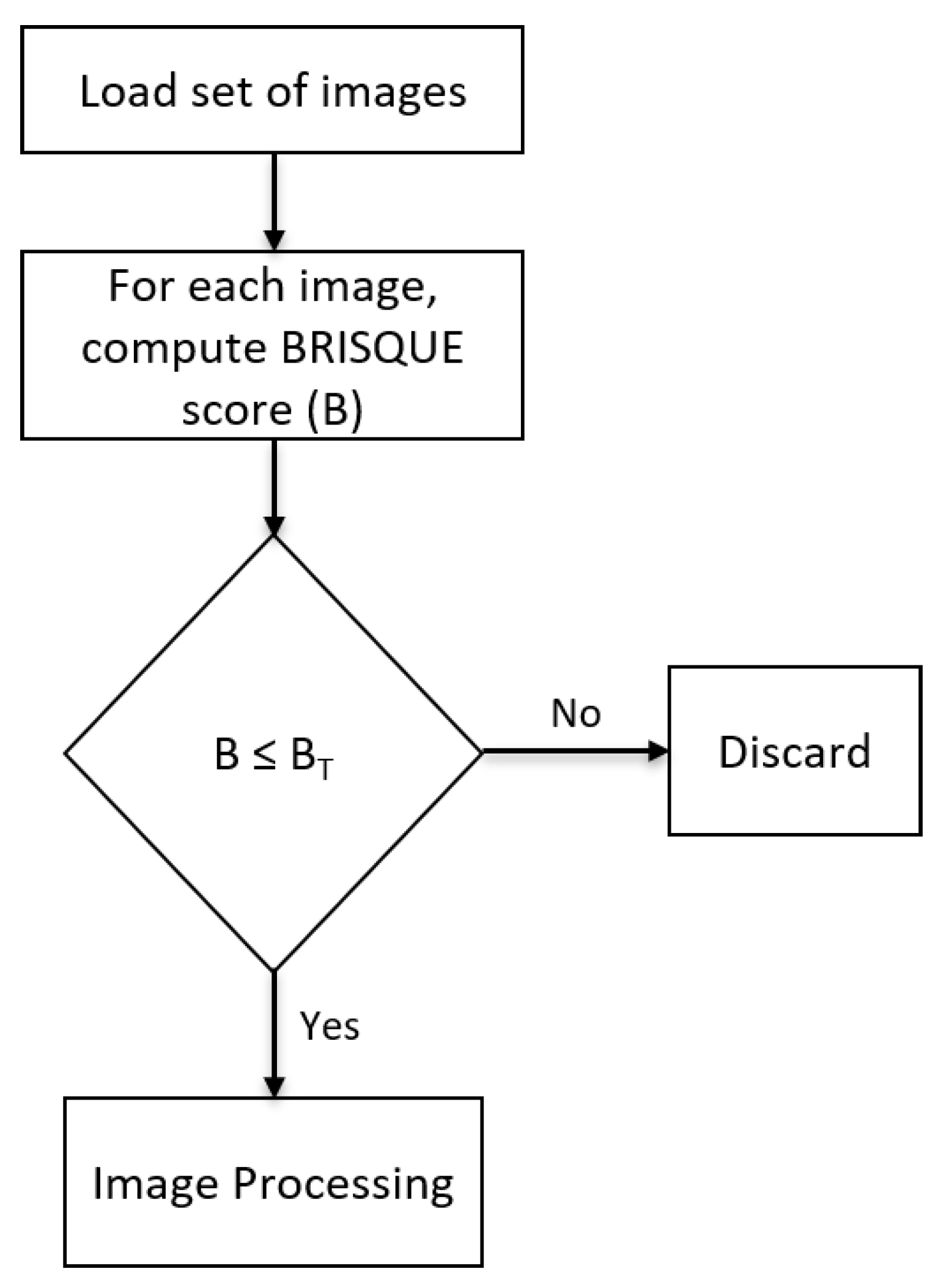
To enhance the quality of images utilised for training and testing, it is crucial to carry out data cleaning by removing low-quality images, ultimately saving time. The block diagram presented in
Figure 13 illustrates the process of BRISQUE-based data cleaning of images. The algorithm initially loads images, computes the BRISQUE scores (B) for each image, and compares them to a pre-defined threshold value. The BRISQUE score threshold (B
) is determined based on the specific task requirements. If the BRISQUE score of the image surpasses the set threshold, the image is discarded; otherwise, it is retained for further image processing. By eliminating low-quality images, i.e., images with higher BRISQUE scores, the performance and accuracy of the deep learning model can be improved, ensuring that the dataset contains only high-quality images.
5. Conclusions and Future Work
It is crucial to assess image quality when detecting and categorising concrete cracks. This study explored the correlation between the BRISQUE-IQA method and the VGG16 crack classification model. The results indicate that the VGG16 model performs best when trained and tested on clean datasets than degraded datasets containing Gaussian noise and blur. The evaluation using BRISQUE scores showed that as the noise or blur in the image increased, the BRISQUE score also increased, indicating a decrease in image quality. Therefore, it is essential to carefully preprocess data and select appropriate metrics and models when developing image processing algorithms.
The study also emphasized the crucial importance of data cleaning within the BRISQUE score threshold and its significant role in enhancing model adaptability and performance in diverse image quality scenarios. These findings open new avenues for developing image-based inspection systems, providing valuable contributions to fields that rely on precise image analysis. The BRISQUE score threshold (B) effectively evaluated image quality and enhanced the model’s classification accuracy.
Incorporating the implemented methodology into the data preprocessing stage reduces the computation burden of processing low-quality images. It also helps in improving the efficiency of the crack detection and classification process, resulting in faster training and testing times and reduced computational costs. The results of this study have important implications for improving the precision and dependability of automated visual inspection systems used to detect concrete cracks and monitor structural health. Moreover, this knowledge can be applied to diverse fields, including medical imaging and face recognition, where high-quality images are critical for accurate diagnoses. Furthermore, the proposed BRISQUE-assisted deep learning approach can quickly screen vast surface areas of concrete structures such as airport runways and highway pavements.
As part of our future research, we plan to expand our dataset by including a broader range of concrete images that contain various real-world confounding variables (e.g., bio-fouling, efflorescence, corrosion, spalling) and conduct an extensive comparative analysis of various image classification networks, including VGG-16, ResNet, Inception, Xception, and others, for concrete image quality assessment.
Author Contributions
S.P.: Conceptualization, Data curation, Methodology, Visualization, Validation, Software, Writing—original draft, Writing—review and editing. M.P.: Funding acquisition, Supervision, Resources, Writing—review and editing. J.M.: Data curation, Writing—review and editing. H.D.: Writing—review and editing. G.D.: Supervision. All authors have read and agreed to the published version of the manuscript.
Funding
This document is the results of the research project funded by the Scottish Funding Council (BE-ST and CENSIS Innovation Centre) and the University of Strathclyde’s Advanced Nuclear Research Centre.
Institutional Review Board Statement
Not applicable.
Informed Consent Statement
Not applicable.
Data Availability Statement
The data that has been used in this study is confidential and is unavailable due to privacy or ethical restrictions.
Acknowledgments
The authors would like to express gratitude to the Civil and Environmental Engineering department of University of Strathclyde for their generous support.
Conflicts of Interest
The authors declare that they have no known competing financial interests or personal relationships that could have appeared to influence the work reported in this paper.
References
- Chang, P.C.; Flatau, A.; Liu, S.C. Review Paper: Health Monitoring of Civil Infrastructure. Struct. Health Monit. 2003, 2, 257–267. [Google Scholar] [CrossRef]
- Farrar, C.R.; Worden, K. An Introduction to Structural Health Monitoring. In New Trends in Vibration Based Structural Health Monitoring; Deraemaeker, A., Worden, K., Eds.; Springer: Vienna, Austria, 2010; pp. 1–17. [Google Scholar] [CrossRef]
- Abedin, S.; Biondi, A.M.; Wu, R.; Cao, L.; Wang, X. Structural health monitoring using a new type of distributed fiber optic smart textiles in combination with optical frequency domain reflectometry (OFDR): Taking a pedestrian bridge as case study. Sensors 2023, 23, 1591. [Google Scholar] [CrossRef] [PubMed]
- Flah, M.; Suleiman, A.R.; Nehdi, M.L. Classification and quantification of cracks in concrete structures using deep learning image-based techniques. Cem. Concr. Compos. 2020, 114, 103781. [Google Scholar] [CrossRef]
- Zhou, Z.; Zhang, B.; Xia, K.; Li, X.; Yan, G.; Zhang, K. Smart film for crack monitoring of concrete bridges. Struct. Health Monit. 2011, 10, 275–289. [Google Scholar] [CrossRef]
- Mishra, M.; Lourenço, P.B.; Ramana, G.V. Structural health monitoring of civil engineering structures by using the internet of things: A review. J. Build. Eng. 2022, 48, 103954. [Google Scholar] [CrossRef]
- Gehri, N.; Mata-Falcón, J.; Kaufmann, W. Automated crack detection and measurement based on digital image correlation. Constr. Build. Mater. 2020, 256, 119383. [Google Scholar] [CrossRef]
- Agnisarman, S.; Lopes, S.; Madathil, K.C.; Piratla, K.; Gramopadhye, A. A survey of automation-enabled human-in-the-loop systems for infrastructure visual inspection. Autom. Constr. 2019, 97, 52–76. [Google Scholar] [CrossRef]
- Chow, J.K.; Liu, K.F.; Tan, P.S.; Su, Z.; Wu, J.; Li, Z.; Wang, Y.H. Automated defect inspection of concrete structures. Autom. Constr. 2021, 132, 103959. [Google Scholar] [CrossRef]
- Guo, Y.; Shen, X.; Linke, J.; Wang, Z.; Barati, K. Quantification of Structural Defects Using Pixel Level Spatial Information from Photogrammetry. Sensors 2023, 23, 5878. [Google Scholar] [CrossRef]
- Pennada, S.; Perry, M.; McAlorum, J.; Dow, H.; Dobie, G. Performance evaluation of an improved deep CNN-based concrete crack detection algorithm. In Proceedings of the Society of Photo-Optical Instrumentation Engineers (SPIE) Conference Series, Long Beach, CA, USA, 12–16 March 2023; Volume 12486, p. 1248615. [Google Scholar] [CrossRef]
- Golding, V.P.; Gharineiat, Z.; Munawar, H.S.; Ullah, F. Crack Detection in Concrete Structures Using Deep Learning. Sustainability 2022, 14, 8117. [Google Scholar] [CrossRef]
- Sony, S.; Dunphy, K.; Sadhu, A.; Capretz, M. A systematic review of convolutional neural network-based structural condition assessment techniques. Eng. Struct. 2021, 226, 111347. [Google Scholar] [CrossRef]
- Dorafshan, S.; Thomas, R.J.; Maguire, M. Comparison of deep convolutional neural networks and edge detectors for image-based crack detection in concrete. Constr. Build. Mater. 2018, 186, 1031–1045. [Google Scholar] [CrossRef]
- Seol, D.H.; Oh, J.H.; Kim, H.J. Comparison of deep learning-based CNN models for crack detection. J. Archit. Inst. Korea Struct. Constr. 2020, 36, 113–120. [Google Scholar] [CrossRef]
- McAlorum, J.; Perry, M.; Dow, H.; Pennada, S. Robotic concrete inspection with illumination-enhancement. In Proceedings of the Sensors and Smart Structures Technologies for Civil, Mechanical, and Aerospace Systems, Long Beach, CA, USA, 12–16 March 2023; Volume 12486, pp. 125–131. [Google Scholar] [CrossRef]
- Dodge, S.; Karam, L. Understanding how image quality affects deep neural networks. In Proceedings of the 2016 Eighth International Conference on Quality of Multimedia Experience (QoMEX), Lisbon, Portugal, 6–8 June 2016; pp. 1–6. [Google Scholar] [CrossRef]
- Mittal, A.; Moorthy, A.K.; Bovik, A.C. No-Reference Image Quality Assessment in the Spatial Domain. IEEE Trans. Image Process. 2012, 21, 4695–4708. [Google Scholar] [CrossRef]
- Lattanzi, D.; Miller, G. Review of Robotic Infrastructure Inspection Systems. J. Infrastruct. Syst. 2017, 23, 04017004. [Google Scholar] [CrossRef]
- Mei, Q.; Gül, M. A cost effective solution for pavement crack inspection using cameras and deep neural networks. Constr. Build. Mater. 2020, 256, 119397. [Google Scholar] [CrossRef]
- Tse, K.W.; Pi, R.; Sun, Y.; Wen, C.Y.; Feng, Y. A Novel Real-Time Autonomous Crack Inspection System Based on Unmanned Aerial Vehicles. Sensors 2023, 23, 3418. [Google Scholar] [CrossRef] [PubMed]
- Hou, W.; Gao, X.; Tao, D.; Li, X. Blind image quality assessment via deep learning. IEEE Trans. Neural Networks Learn. Syst. 2014, 26, 1275–1286. [Google Scholar] [CrossRef]
- Barman, S.A.; Welikala, R.A.; Rudnicka, A.R.; Owen, C.G. Image quality assessment. In Computational Retinal Image Analysis; Elsevier: Amsterdam, The Netherlands, 2019; pp. 135–155. [Google Scholar] [CrossRef]
- Wang, Z. Applications of Objective Image Quality Assessment Methods [Applications Corner]. IEEE Signal Process. Mag. 2011, 28, 137–142. [Google Scholar] [CrossRef]
- Lin, H.I.; Wibowo, F.S. Image Data Assessment Approach for Deep Learning-Based Metal Surface Defect-Detection Systems. IEEE Access 2021, 9, 47621–47638. [Google Scholar] [CrossRef]
- Mohammadi, P.; Ebrahimi-Moghadam, A.; Shirani, S. Subjective and Objective Quality Assessment of Image: A Survey. arXiv 2014. [Google Scholar] [CrossRef]
- Chow, L.S.; Paramesran, R. Review of medical image quality assessment. Biomed. Signal Process. Control 2016, 27, 145–154. [Google Scholar] [CrossRef]
- Chandra Mohan, T. Blind Image Quality Assessment of Smartphone-Captured Images in the Wild. 2021. Available online: http://essay.utwente.nl/89267/ (accessed on 5 March 2023).
- Bosse, S.; Maniry, D.; Müller, K.R.; Wiegand, T.; Samek, W. Deep Neural Networks for No-Reference and Full-Reference Image Quality Assessment. IEEE Trans. Image Process. 2018, 27, 206–219. [Google Scholar] [CrossRef] [PubMed]
- Wang, L. A survey on IQA. arXiv 2022. [Google Scholar] [CrossRef]
- Xu, S.; Jiang, S.; Min, W. No-reference/Blind Image Quality Assessment: A Survey. IETE Tech. Rev. 2017, 34, 223–245. [Google Scholar] [CrossRef]
- Varga, D. No-Reference Image Quality Assessment Using the Statistics of Global and Local Image Features. Electronics 2023, 12, 1615. [Google Scholar] [CrossRef]
- Kim, B.; Choi, S.W.; Hu, G.; Lee, D.E.; Serfa Juan, R.O. Multivariate Analysis of Concrete Image Using Thermography and Edge Detection. Sensors 2021, 21, 7396. [Google Scholar] [CrossRef] [PubMed]
- Siriwardana, E.; Amila, S.K.; Kaushalya, S.; Chandrasiri, S.; Piyawardana, V.S. Driving Through a Bend: Detection of Unsafe Driving Patterns and Prevention of Heavy Good Vehicle Rollovers. In Proceedings of the 2021 2nd International Informatics and Software Engineering Conference (IISEC), Ankara, Turkey, 16–17 December 2021; pp. 1–6. [Google Scholar] [CrossRef]
- Ichi, E.; Dorafshan, S. Effectiveness of infrared thermography for delamination detection in reinforced concrete bridge decks. Autom. Constr. 2022, 142, 104523. [Google Scholar] [CrossRef]
- Rahman, E.U.; Zhang, Y.; Ahmad, S.; Ahmad, H.I.; Jobaer, S. Autonomous vision-based primary distribution systems porcelain insulators inspection using UAVs. Sensors 2021, 21, 974. [Google Scholar] [CrossRef]
- Simonyan, K.; Zisserman, A. Very deep convolutional networks for large-scale image recognition. arXiv 2014, arXiv:1409.1556. [Google Scholar] [CrossRef]
- Deng, J.; Dong, W.; Socher, R.; Li, L.J.; Li, K.; Li, F.-F. ImageNet: A large-scale hierarchical image database. In Proceedings of the 2009 IEEE Conference on Computer Vision and Pattern Recognition, Miami, FL, USA, 20–25 June 2009; pp. 248–255. [Google Scholar] [CrossRef]
- EN 1992-1-1: Eurocode 2: Design of Concrete Structures—Part 1-1: General Rules and Rules for Buildings, Section 7.3.1: Crack Control, [Authority: The European Union Per Regulation 305/2011, Directive 98/34/EC, Directive 2004/18/EC]. 2004. Available online: https://www.phd.eng.br/wp-content/uploads/2015/12/en.1992.1.1.2004.pdf (accessed on 5 February 2021).
- Takmanman. Gaussian Noise and Gaussian Filter. 2020. Available online: https://takmanman.github.io/2020/05/23/gaussian-noise-gaussian-filter.html (accessed on 17 August 2022).
- Robinson, P.E.; Roodt, Y. Blind deconvolution of Gaussian blurred images containing additive white Gaussian noise. In Proceedings of the 2013 IEEE International Conference on Industrial Technology (ICIT), Cape Town, South Africa, 25–28 February 2013; pp. 1092–1097. [Google Scholar] [CrossRef]
- Weiss, K.; Khoshgoftaar, T.M.; Wang, D. A survey of transfer learning. J. Big Data 2016, 3, 1–40. [Google Scholar] [CrossRef]
- Yosinski, J.; Clune, J.; Bengio, Y.; Lipson, H. How transferable are features in deep neural networks? arXiv 2014. [Google Scholar] [CrossRef]
- Liu, X.; Chi, M.; Zhang, Y.; Qin, Y. Classifying high resolution remote sensing images by fine-tuned VGG deep networks. In Proceedings of the IGARSS 2018 IEEE International Geoscience and Remote Sensing Symposium, Valencia, Spain, 22–27 July 2018; pp. 7137–7140. [Google Scholar] [CrossRef]
- Yang, Z.; Yue, J.; Li, Z.; Zhu, L. Vegetable image retrieval with fine-tuning VGG model and image hash. IFAC-PapersOnLine 2018, 51, 280–285. [Google Scholar] [CrossRef]
- Kingma, D.P.; Ba, J. Adam: A method for stochastic optimization. arXiv 2014, arXiv:1412.6980. [Google Scholar] [CrossRef]
- Wardhani, N.W.S.; Rochayani, M.Y.; Iriany, A.; Sulistyono, A.D.; Lestantyo, P. Cross-validation metrics for evaluating classification performance on imbalanced data. In Proceedings of the 2019 International Conference on Computer, Control, Informatics and Its Applications (IC3INA), Tangerang, Indonesia, 23–24 October 2019; pp. 14–18. [Google Scholar] [CrossRef]
- Sthle, L.; Wold, S. Analysis of variance (ANOVA). Chemom. Intell. Lab. Syst. 1989, 6, 259–272. [Google Scholar] [CrossRef]
Figure 1.
Workflow overview of threshold-based BRISQUE-assisted deep learning for enhancing crack detection in concrete structures.
Figure 1.
Workflow overview of threshold-based BRISQUE-assisted deep learning for enhancing crack detection in concrete structures.
Figure 2.
Comparison of image quality using BRISQUE scores. (a) Natural image with a BRISQUE score of 24.91, indicating better image quality. (b) Noisy image with a BRISQUE score of 71.05, indicating poor image quality.
Figure 2.
Comparison of image quality using BRISQUE scores. (a) Natural image with a BRISQUE score of 24.91, indicating better image quality. (b) Noisy image with a BRISQUE score of 71.05, indicating poor image quality.
Figure 3.
Specialized inspection equipment with single adjustable arm for 50-degree lighting projection onto concrete surface.
Figure 3.
Specialized inspection equipment with single adjustable arm for 50-degree lighting projection onto concrete surface.
Figure 4.
Illustration of variables during image capture. Light from an imaged object passes through the lens and aperture onto the camera sensor.
Figure 4.
Illustration of variables during image capture. Light from an imaged object passes through the lens and aperture onto the camera sensor.
Figure 5.
(a) Baseline (pristine) image. (b) Colour map of pristine image (the lighter the pixels, the better the image quality).
Figure 5.
(a) Baseline (pristine) image. (b) Colour map of pristine image (the lighter the pixels, the better the image quality).
Figure 6.
(a) Noisy image of noise factor 50. (b) Colour map of noisy image (the lighter the pixels, the better the image quality).
Figure 6.
(a) Noisy image of noise factor 50. (b) Colour map of noisy image (the lighter the pixels, the better the image quality).
Figure 7.
(a) Blurred image of blur factor 8. (b) Colour map of blurred image (the lighter the pixels, the better the image quality).
Figure 7.
(a) Blurred image of blur factor 8. (b) Colour map of blurred image (the lighter the pixels, the better the image quality).
Figure 8.
VGG16 crack classification model.
Figure 8.
VGG16 crack classification model.
Figure 9.
Comparison of BRISQUE scores for various levels of noise and blur in image processing.
Figure 9.
Comparison of BRISQUE scores for various levels of noise and blur in image processing.
Figure 10.
Performance comparison of VGG16 neural network model on Noisy images using accuracy, F1 score, and Matthew’s correlation coefficient metrics.
Figure 10.
Performance comparison of VGG16 neural network model on Noisy images using accuracy, F1 score, and Matthew’s correlation coefficient metrics.
Figure 11.
Performance comparison of VGG16 neural network model on Blurred images using accuracy, F1 score, and Matthew’s correlation coefficient metrics.
Figure 11.
Performance comparison of VGG16 neural network model on Blurred images using accuracy, F1 score, and Matthew’s correlation coefficient metrics.
Figure 12.
Performance comparison of VGG16 neural network model on images with different BRISQUE score thresholds using accuracy, F1 score, and Matthew’s correlation coefficient metrics.
Figure 12.
Performance comparison of VGG16 neural network model on images with different BRISQUE score thresholds using accuracy, F1 score, and Matthew’s correlation coefficient metrics.
Figure 13.
BRISQUE-based data cleaning, where B and B represent the BRISQUE score and BRISQUE score threshold, respectively.
Figure 13.
BRISQUE-based data cleaning, where B and B represent the BRISQUE score and BRISQUE score threshold, respectively.
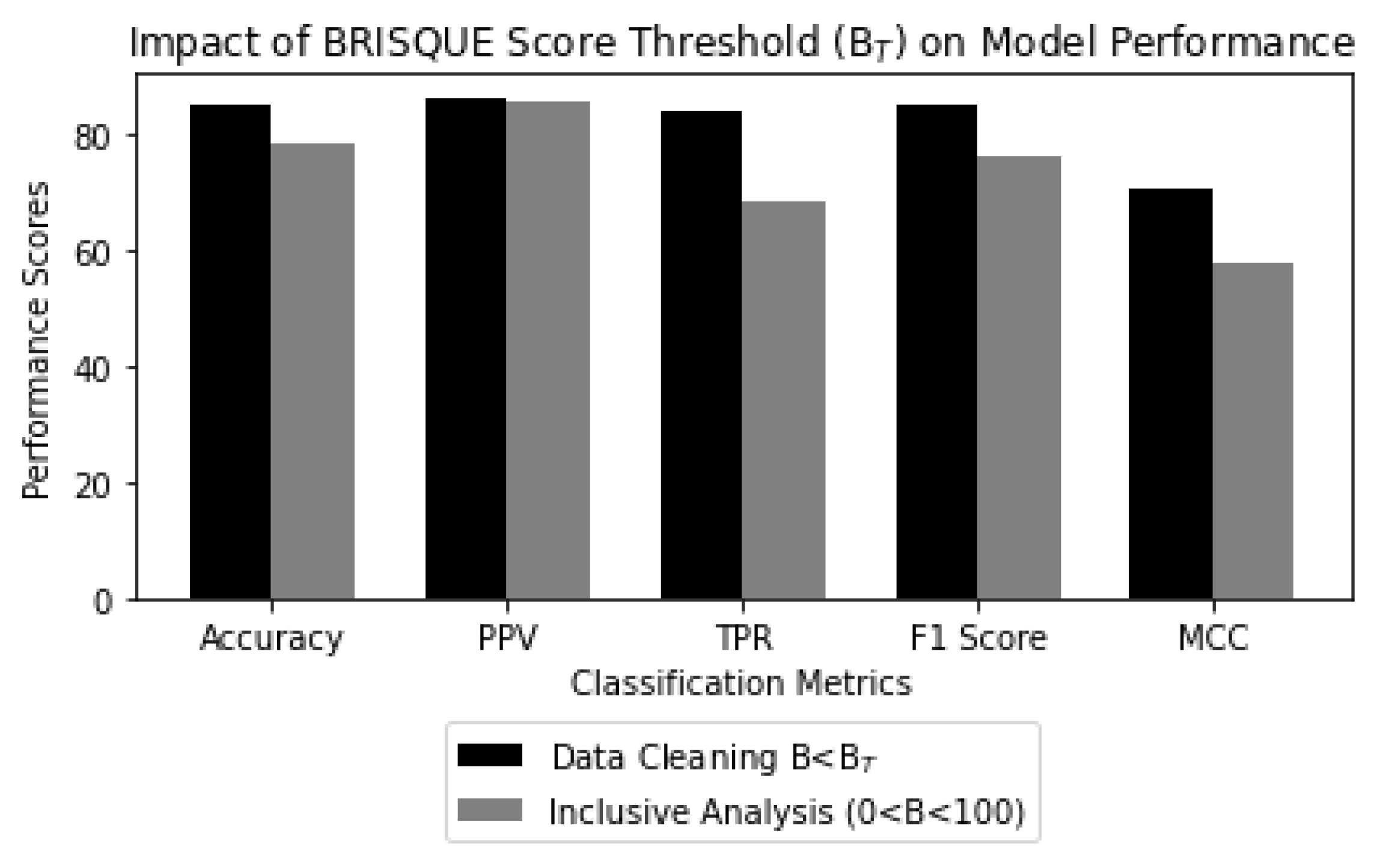
Figure 14.
Impact of BRISQUE score threshold (B) on model performance, where Data Cleaning indicates that the trained model is tested on images within the BRISQUE score threshold, i.e., B < B, and Inclusive Analysis indicates that the testing dataset includes all images, both within and surpassing the BRISQUE score threshold, i.e., 0 < B < 100.
Table 1.
Performance metrics of a binary classifier.
Table 1.
Performance metrics of a binary classifier.
| Name | Description | Equation |
|---|
| True Positive Rate (TPR) | The ratio of correctly predicted positive instances to the total number of actual positive instances. | |
| Positive Predictive Value (PPV) | The ratio of correctly predicted positive instances to the total number of positive predictions. | |
| F1 Score | The weighted average of recall and precision. | |
| Accuracy | The measure of the model’s ability to correctly predict the outcomes. | |
| Matthew’s Correlation Coefficient (MCC) | The measure of the correlation between predicted and actual labels, accounting for true or false, both positive and negative predictions. | |
Table 2.
Testing matrix.
| | Train on
Noisy | Train on
Blur | Train on
Pristine |
|---|
Test on
Noisy | x | | x |
Test on
Blur | | x | x |
Test on
Pristine | | | x |
Table 3.
Testing matrix when the model is trained and tested on noisy images.
Table 3.
Testing matrix when the model is trained and tested on noisy images.
| | Train on
Noisy | Train on
Pristine |
|---|
Test on
Noisy | x | x |
Test on
Pristine | | x |
Table 4.
Testing matrix when the model is trained and tested on blurred images.
Table 4.
Testing matrix when the model is trained and tested on blurred images.
| | Train on
Blur | Train on
Pristine |
|---|
Test on
Blur | x | x |
Test on
Pristine | | x |
Table 5.
Comparison of model performance at different BRISQUE score threshold values.
Table 5.
Comparison of model performance at different BRISQUE score threshold values.
BRISQUE
Scores | Number of
Training
Images | Accuracy | F1 Score | MCC |
|---|
| <45 | 360 | 0.8 | 0.77 | 0.61 |
| <55 | 720 | 0.66 | 0.73 | 0.40 |
| <65 | 2160 | 0.73 | 0.76 | 0.49 |
| <75 | 3240 | 0.73 | 0.66 | 0.48 |
| <85 | 3960 | 0.61 | 0.69 | 0.30 |
| Disclaimer/Publisher’s Note: The statements, opinions and data contained in all publications are solely those of the individual author(s) and contributor(s) and not of MDPI and/or the editor(s). MDPI and/or the editor(s) disclaim responsibility for any injury to people or property resulting from any ideas, methods, instructions or products referred to in the content. |
© 2023 by the authors. Licensee MDPI, Basel, Switzerland. This article is an open access article distributed under the terms and conditions of the Creative Commons Attribution (CC BY) license (https://creativecommons.org/licenses/by/4.0/).


